Investigating the Impact of E-Mobility on the Electrical Power Grid Using a Simplified Grid Modelling Approach


Abstract
1. Introduction
2. Methods
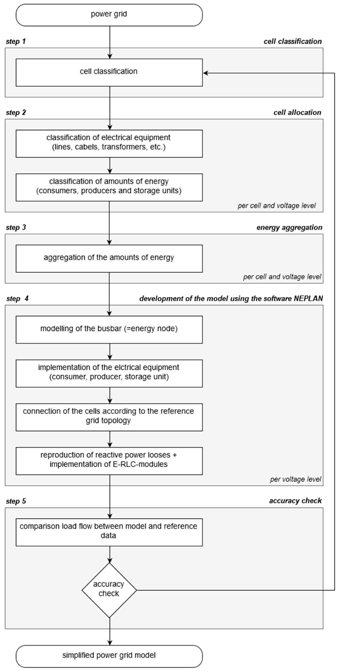
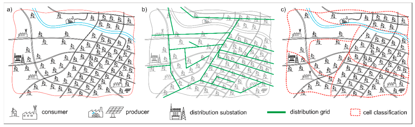
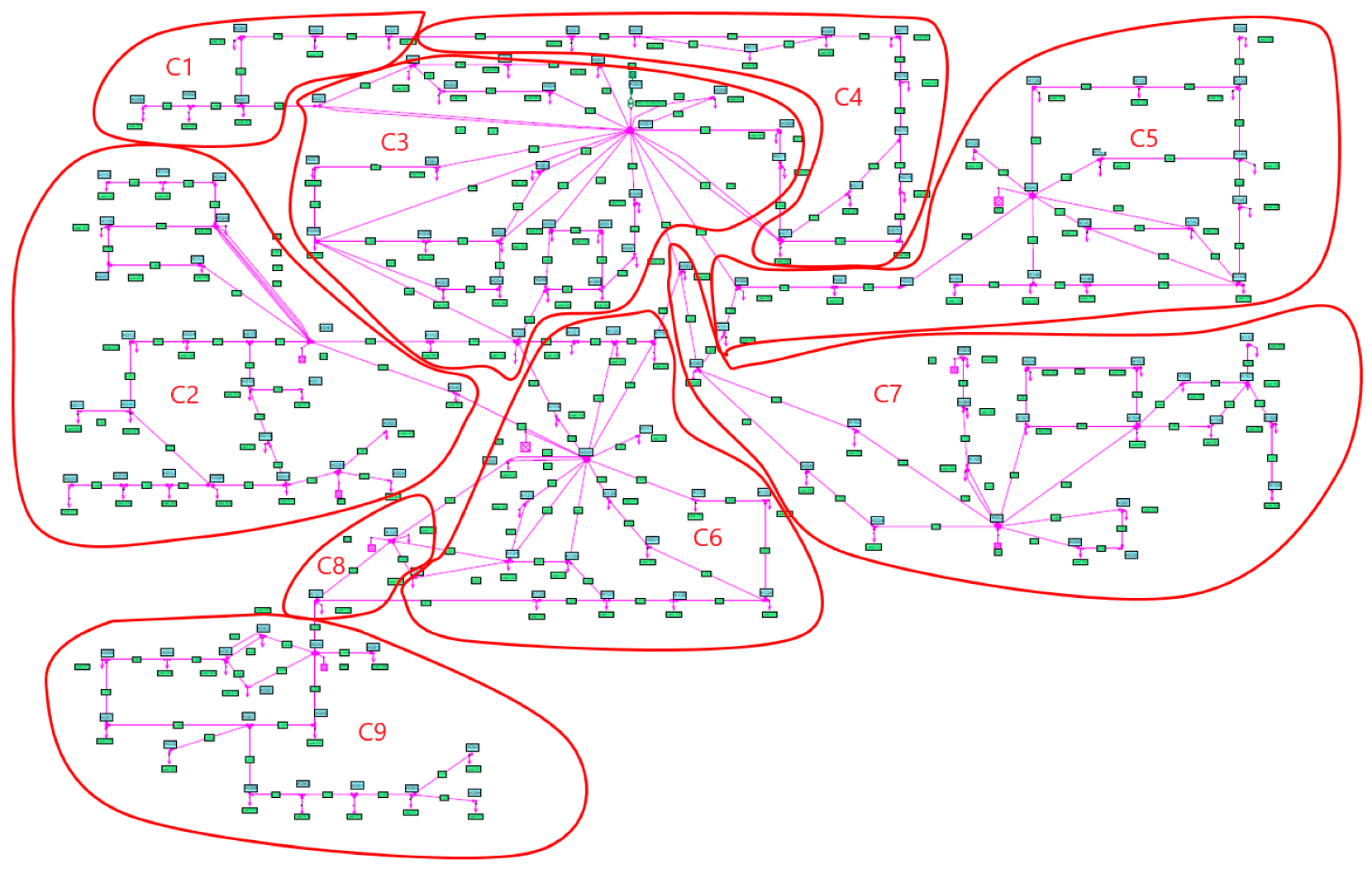
2.1. Development of Simplified Distribution Grid Models Based on a Cellular Approach
- Consideration of grid topology before geographic topology.
- Resulting grid model should correspond to a radial grid.
- Prevention of closed ring structure (use of lines with normally open points to connect two cells with each other).
- Existing rings in the reference grid should be combined in one cell.
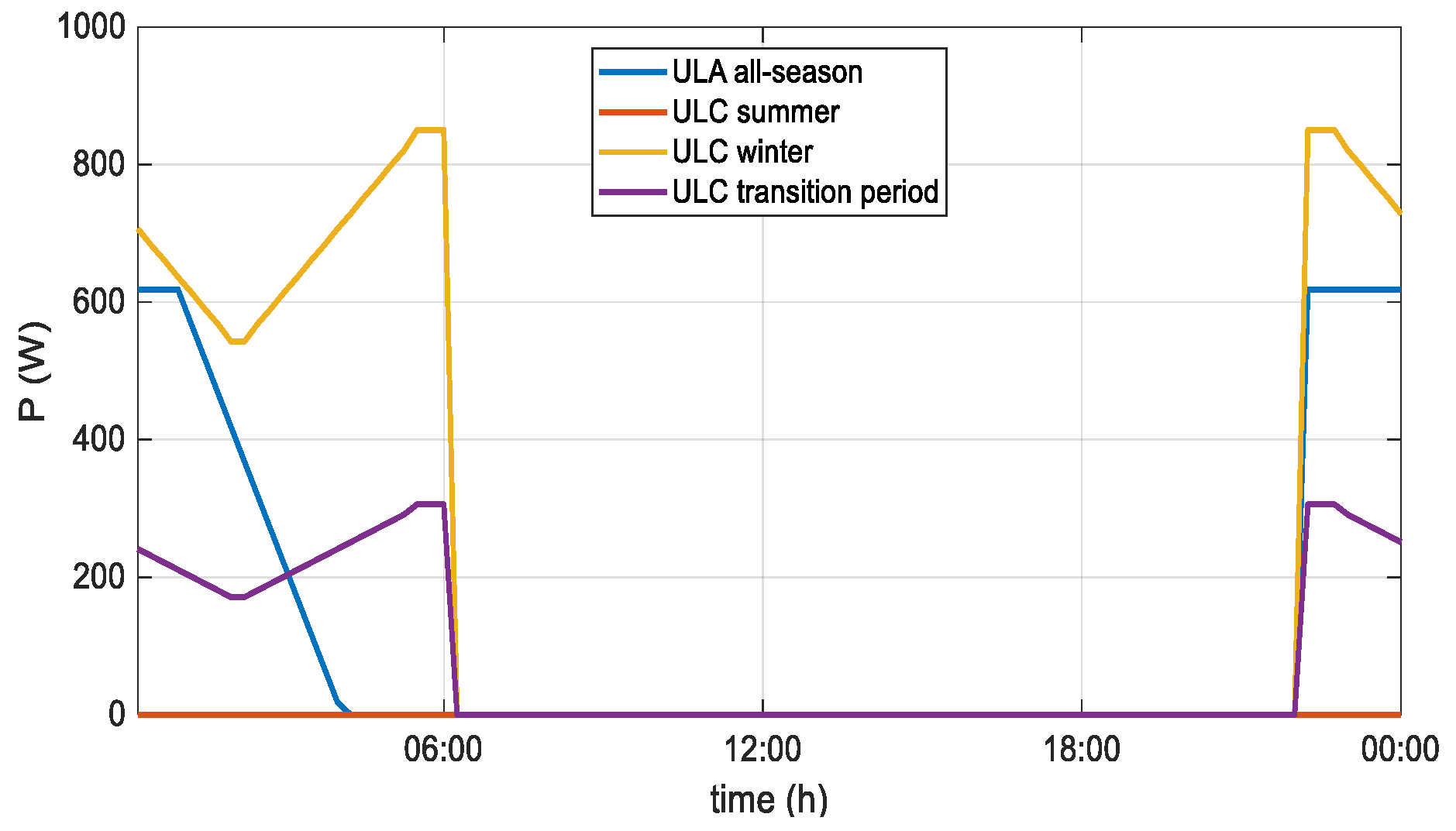
2.2. Determination of Load and Production Profiles
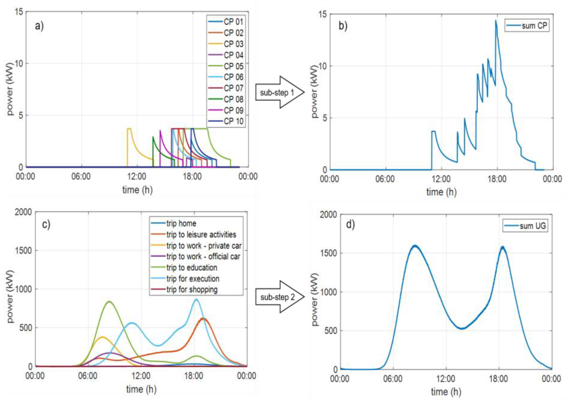
2.3. Determination of Synthetic Charging Load Profiles of Electric Vehicles
- In charging strategy 1, the charging power is selected separately for each user group. All charging processes within a user group thus charge with the same charging power. For example, as is quite common with today’s charging stations, charging powers can vary between 3.7 and 50 kW.
- For charging strategy 2, the charging power is determined for each charging process based on a probability distribution function. This distribution function can, for example, be determined from the data of charging stations and therefore describes how many users have charged with which charging power.
- Charging strategy 3 simulates the possibility of reduced charging power under consideration of the available charging time, corresponding to the duration of stay. The determination of the reduced charging power takes place in step 3. Since each loading process is simulated independently of the previous or subsequent one, it is not possible at this point to shift the charging process within the duration of stay as part of this strategy. The influence on the time shift would have to be taken into account when preparing the distributions for arrival and departure times.
3. Results and Discussion
3.1. Calculation Times
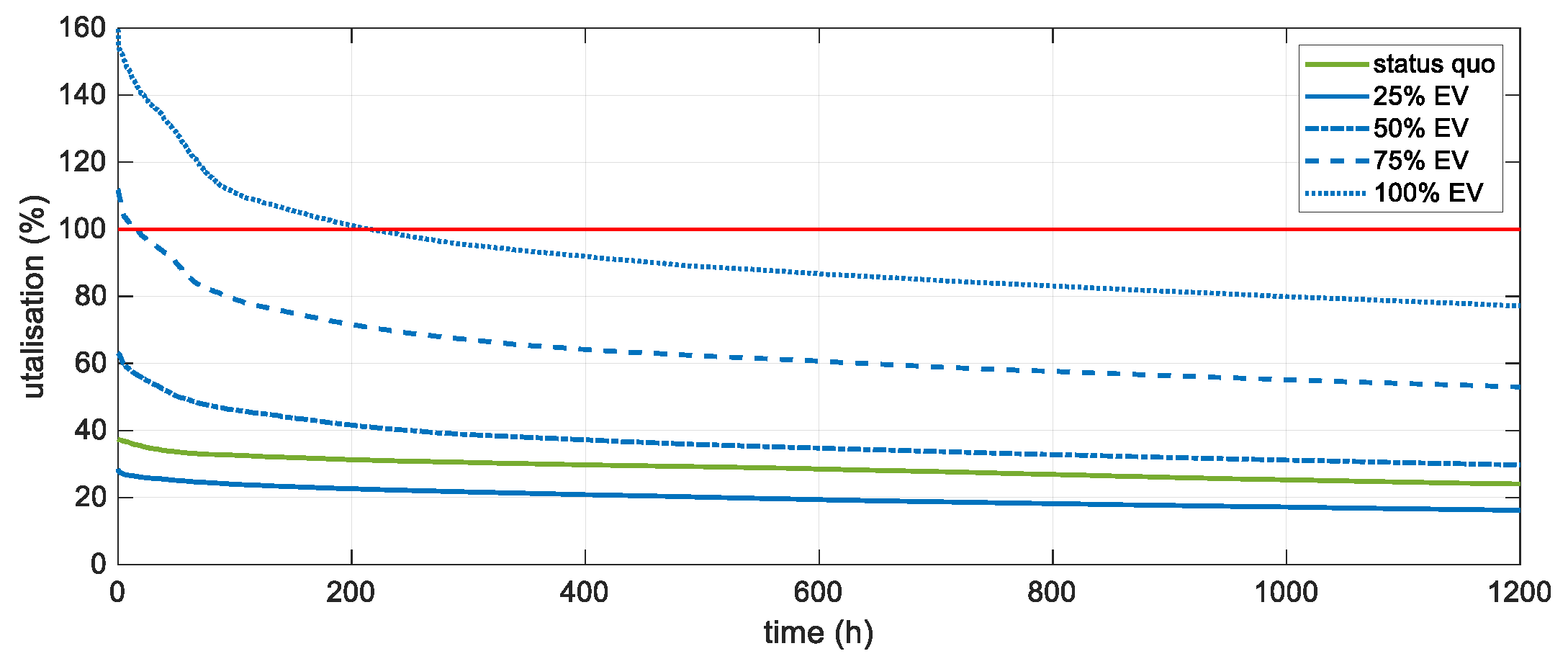
3.2. Case Study: Impact of E-Mobility Integration
4. Conclusions
Author Contributions
Funding
Conflicts of Interest
References
- Meinshausen, M.; Meinshausen, N.; Hare, W.; Raper, S.C.B.; Frieler, K.; Knutti, R.; Frame, D.J.; Allen, M.R. Greenhouse-gas emission targets for limiting global warming to 2 °C. Nature 2009, 458, 1158–1162. [Google Scholar] [CrossRef] [PubMed]
- Raftery, A.E.; Zimmer, A.; Frierson, D.M.W.; Startz, R.; Liu, P. Less than 2 °C warming by 2100 unlikely. Nclimate 2017, 7, 637–641. [Google Scholar] [CrossRef] [PubMed]
- Bundesministerium für Wissenschaft, Forschung und Wirtschaft. Energ. Österr. Zahl. Daten Fakten 2017, 6.
- Statistik Austria. Kraftfahrzeuge—Neuzulassungen. Available online: http://www.statistik.at/web_de/statistiken/energie_umwelt_innovation_mobilitaet/verkehr/strasse/kraftfahrzeuge_-_neuzulassungen/index.html (accessed on 30 September 2019).
- Clement-Nyns, K.; Haesen, E.; Driesen, J. The Impact of Charging Plug-In Hybrid Electric Vehicles on a Residential Distribution Grid. IEEE Trans. Power Syst. 2010, 25, 371–380. [Google Scholar] [CrossRef]
- Valsera Naranjo, E.; Sumper, A.; Lloret Gallego, P.; Villafáfila Robles, R.; Sudrià Andreu, A. Deterministic and Probabilistic Assessment of the Impact of the Electrical Vehicles on the Power Grid. REPQJ 2010, 1, 1505–1509. [Google Scholar] [CrossRef]
- Chandra Mouli, G.R.; Bauer, P.; Zeman, M. System design for a solar powered electric vehicle charging station for workplaces. Appl. Energy 2016, 168, 434–443. [Google Scholar] [CrossRef]
- Fattori, F.; Anglani, N.; Muliere, G. Combining photovoltaic energy with electric vehicles, smart charging and vehicle-to-grid. Sol. Energy 2014, 110, 438–451. [Google Scholar] [CrossRef]
- Fischer, D.; Harbrecht, A.; Surmann, A.; McKenna, R. Electric vehicles’ impacts on residential electric local profiles—A stochastic modelling approach considering socio-economic, behavioural and spatial factors. Appl. Energy 2019, 233, 644–658. [Google Scholar] [CrossRef]
- Iversen, E.B.; Morales, J.M.; Madsen, H. Optimal charging of an electric vehicle using a Markov decision process. Appl. Energy 2014, 123, 1–12. [Google Scholar] [CrossRef]
- Olivella-Rosell, P.; Villafafila-Robles, R.; Sumper, A.; Bergas-Jané, J. Probabilistic Agent-Based Model of Electric Vehicle Charging Demand to Analyse the Impact on Distribution Networks. Energies 2015, 8, 4160–4187. [Google Scholar] [CrossRef]
- Neaimeh, M.; Wardle, R.; Jenkins, A.M.; Yi, J.; Hill, G.; Lyons, P.F.; Hübner, Y.; Blythe, P.T.; Taylor, P.C. A probabilistic approach to combining smart meter and electric vehicle charging data to investigate distribution network impacts. Appl. Energy 2015, 157, 688–698. [Google Scholar] [CrossRef]
- Leou, R.C.; Su, C.L.; Lu, C.N. Stochastic Analyses of Electric Vehicle Charging Impacts on Distribution Network. IEEE Trans. Power Syst. 2014, 29, 1055–1063. [Google Scholar] [CrossRef]
- Gnann, T.; Funke, S.; Jakobsson, N.; Plötz, P.; Sprei, F.; Bennehag, A. Fast charging infrastructure for electric vehicles: Today’s situation and future needs. Transp. Res. Part D 2018, 62, 314–329. [Google Scholar] [CrossRef]
- Godde, M.; Findeisen, T.; Sowa, T.; Nguyen, P.H. Modelling the charging probability of electric vehicles as a gaussian mixture model for a convolution based power flow analysis. In Proceedings of the 2015 IEEE Eindhoven PowerTech, Eindhoven, The Netherlands, 29 June–2 July 2015; pp. 1–6, ISBN 978-1-4799-7693-5. [Google Scholar]
- Mobilität in Deutschland—MiD Ergebnisbericht; Infas—Institut für Angewandte Sozialwissenschaften GmbH; Deutsches Zentrum für Luftund Raumfahrt e.V. Institut für Verkehrsforschung; IVT Research GmbH; Bundesministerium für Verkehr und digitale Infrastruktur: Bonn, Germany, 2018.
- Lin, H.; Fu, K.; Liu, Y.; Sun, Q.; Wennersten, R. Modeling charging demand of electric vehicles in multi-locations using agent-based method. Energy Procedia 2018, 152, 599–605. [Google Scholar] [CrossRef]
- Wang, D.; Gao, J.; Li, P.; Wang, B.; Zhang, C.; Saxena, S. Modeling of plug-in electric vehicle travel patterns and charging load based on trip chain generation. J. Power Sources 2017, 359, 468–479. [Google Scholar] [CrossRef]
- Darabi, Z.; Ferdowsi, M. Aggregated Impact of Plug-in Hybrid Electric Vehicles on Electricity Demand Profile. IEEE Trans. Sustain. Energy 2011, 2, 501–508. [Google Scholar] [CrossRef]
- Garcia-Villalobos, J.; Zamora, I.; Eguia, P.; San Martin, J.I.; Asensio, F.J. Modelling social patterns of plug-in electric vehicles drivers for dynamic simulations. In Proceedings of the 2014 IEEE International Electric Vehicle Conference (IEVC), Florence, Italy, 17–19 December 2014; pp. 1–7, ISBN 978-1-4799-6075-0. [Google Scholar]
- Federal Highway Administration Office of Policy Information. 2017 NHTS Data User Guide. Available online: https://nhts.ornl.gov/ (accessed on 9 December 2019).
- Leou, R.C.; Su, C.L.; Teng, J.H. Modelling and verifying the load behaviour of electric vehicle charging stations based on field measurements. IET Gener. Transm. Distrib. 2015, 9, 1112–1119. [Google Scholar] [CrossRef]
- Qi, Z.; Yang, J.; Jia, R.; Wang, F. Investigating Real-World Energy Consumption of Electric Vehicles: A Case Study of Shanghai. Procedia Comput. Sci. 2018, 131, 367–376. [Google Scholar] [CrossRef]
- Österrreich Unterwegs 2013/2014 Ergebnisbericht; Infas—Institut für Angewandte Sozialwissenschaft GmbH; TRICONSULT—Wirtschaftsanalytische Forschung Gesellschaft m.b.H; HERRY Consult GmbH; Sammer und Partner Zivilingenieur GmbH, ZIS+P Verkehrsplanung; Institut für Verkehrswesen der Universität für Bodenkultur; Bundesministerium für Verkehr, Innovation und Technologie: Wien, Austria, 2016.
- Luo, L.; Gu, W.; Zhou, S.; Huang, H.; Gao, S.; Han, J.; Wu, Z.; Dou, X. Optimal planning of electric vehicle charging stations comprising multi-types of charging facilities. Appl. Energy 2018, 226, 1087–1099. [Google Scholar] [CrossRef]
- Jianfeng, W.; Xiangning, X.; Jian, Z.; Kunyu, L.; Yang, Y.; Shun, T. Charging demand for electric vehicle based on stochastic analysis of trip chain. IET Gener. Transm. Distrib. 2016, 10, 2689–2698. [Google Scholar] [CrossRef]
- Kazemi, M.A.; Sedighizadeh, M.; Mirzaei, M.J.; Homaee, O. Optimal siting and sizing of distribution system operator owned EV parking lots. Appl. Energy 2016, 179, 1176–1184. [Google Scholar] [CrossRef]
- Qian, K.; Zhou, C.; Allan, M.; Yuan, Y. Modeling of Load Demand Due to EV Battery Charging in Distribution Systems. IEEE Trans. Power Syst. 2011, 26, 802–810. [Google Scholar] [CrossRef]
- Aghaebrahimi, M.R.; Ghasemipour, M.M.; Sedghi, A. Probabilistic optimal placement of EV parking considering different operation strategies. In Proceedings of the MELECON 2014—2014 17th IEEE Mediterranean Electrotechnical Conference, Beirut, Lebanon, 13–16 April 2014; pp. 108–114, ISBN 978-1-4799-2337-3. [Google Scholar]
- Brady, J.; O’Mahony, M. Modelling charging profiles of electric vehicles based on real-world electric vehicle charging data. Sustain. Cities Soc. 2016, 26, 203–216. [Google Scholar] [CrossRef]
- Ul-Haq, A.; Azhar, M.; Mahmoud, Y.; Perwaiz, A.; Al-Ammar, E. Probabilistic Modeling of Electric Vehicle Charging Pattern Associated with Residential Load for Voltage Unbalance Assessment. Energies 2017, 10, 1351. [Google Scholar] [CrossRef]
- Mu, Y.; Wu, J.; Jenkins, N.; Jia, H.; Wang, C. A Spatial–Temporal model for grid impact analysis of plug-in electric vehicles. Appl. Energy 2014, 114, 456–465. [Google Scholar] [CrossRef]
- Grahn, P.; Munkhammar, J.; Widen, J.; Alvehag, K.; Soder, L. PHEV Home-Charging Model Based on Residential Activity Patterns. IEEE Trans. Power Syst. 2013, 28, 2507–2515. [Google Scholar] [CrossRef]
- Grahn, P.; Alvehag, K.; Soder, L. PHEV Utilization Model Considering Type-of-Trip and Recharging Flexibility. IEEE Trans. Smart Grid 2014, 5, 139–148. [Google Scholar] [CrossRef]
- Vopava, J.; Böckl, B.; Kriechbaum, L.; Kienberger, T. Anwendung zellularer Ansätze bei der Gestaltung zukünftiger Energieverbundsysteme. Elektrotech. Inftech. 2017, 134, 238–245. [Google Scholar] [CrossRef]
- Putrus, G.A.; Suwanapingkarl, P.; Johnston, D.; Bentley, E.C.; Narayana, M. Impact of electric vehicles on power distribution networks. In Proceedings of the IEEE Vehicle Power and Propulsion Conference, Dearborn, MI, USA, 7–10 September 2009; pp. 827–831, ISBN 978-1-4244-2600-3. [Google Scholar]
- Shao, S.; Pipattanasomporn, M.; Rahman, S. Challenges of PHEV penetration to the residential distribution network. In Proceedings of the 2009 IEEE PES General Meeting, Calgary, AB, Canada, 26–30 July 2009; pp. 1–8, ISBN 978-1-4244-4241-6. [Google Scholar]
- Böckl, B.; Kriechbaum, L.; Kienberger, T. Analysemethode für kommunale Energiesysteme unter Anwendung des zellularen Ansatzes. In Proceedings of the 14. Symposium Energieinnovation, Graz, Austria, 10–12 February 2016; Institut für Elektrizitätswirtschaft und Energieinnovation: Graz, Austria, 2016. [Google Scholar]
- Böckl, B.; Vopava, J.; Kriechbaum, L.; Kienberger, T. Limitations of integrating photovoltaic energy into municipal grids excluding and including storage systems. In Proceedings of the 6th Solar Integration Workshop, Vienna, Austria, 14–15 November 2016; Energynautics GmbH: Wien, Austria, 2016. [Google Scholar]
- Böckl, B.; Greiml, M.; Leitner, L.; Pichler, P.; Kriechbaum, L.; Kienberger, T. HyFlow—A Hybrid Load Flow-Modelling Framework to Evaluate the Effects of Energy Storage and Sector Coupling on the Electrical Load Flows. Energies 2019, 12, 956. [Google Scholar] [CrossRef]
- QGIS Entwicklungsteam. QGIS Geographisches Informationssystem; 2016. [Google Scholar]
- NEPLAN AG. NEPLAN; 2015. [Google Scholar]
- BDEW—Budesverband der Energie- und Wasserwirtschaft e.V. Standardlastprofile Strom. Available online: https://www.bdew.de/energie/standardlastprofile-strom/ (accessed on 3 April 2019).
- E-CONTROL. Sonstige Marktregeln. Kapitel 6: Zählwerte, Datenformate und Standardisierte Lastprofile. Available online: https://www.e-control.at/recht/marktregeln/sonstige-marktregeln-strom#p_p_id_56_INSTANCE_10318A20066 (accessed on 3 April 2019).
- Esslinger, P.; Witzmann, R. Entwicklung und Verifikation eines stochastischen Verbraucherlastmodells für Haushalte. In Proceedings of the Symposium Energieinnovation, Graz, Austria, 15–17 February 2012; Institut für Elektrizitätswirtschaft und Energieinnovation: Graz, Austria, 2012. [Google Scholar]
- Pflughardt, N. Modellierung von Wasser- und Energieverbräuchen in Haushalten. In Dissertation; Technische Universität Chemnitz: Chemnitz, Germany, 2016. [Google Scholar]
- Pflugradt, N. LoadProfileGenerator. Available online: https://www.loadprofilegenerator.de/ (accessed on 22 November 2019).
- Kraftfahrt-Bundesamt. Neuzulassungen—Deutschland. Available online: https://www.kba.de/DE/Statistik/Fahrzeuge/Neuzulassungen/neuzulassungen_node.html (accessed on 15 July 2019).
- Bosserhoff, D. Integration von Verkehrsplanung und Räumlicher Planung. Teil2: Abschötzung der Verkehrserzeugung Durch Vorhaben der Bauleitungplanung; Hessisches Landesamt für Straßen- und Verkehrswesen: Wiesbaden, Germany, 2000.
- Probst, A.; Braun, M.; Tenbolen, S. Erstellung und Simulation probabilistischer Lastmodelle von Haushalten und Elektrofahrzeugen zur Spannungsbandanalyse; Internationaler ETG-Kongress: Würzburg, Germany, 2011. [Google Scholar]
- Wieland, T.; Reiter, M.; Schmautzer, E.; Fickert, L.; Fabian, J.; Schmied, R. Probabilistische Methode zur Modellierung des Ladeverhaltens von Elektroautos anhand gemessener Daten elektrischer Ladestationen—Auslastungsanalysen von Ladestationen unter Berücksichtigung des Standorts zur Planung von elektrischen Stromnetzen. Elektrotech. Inftech. 2015, 132, 160–167. [Google Scholar] [CrossRef]
- Schuster, A. Batterie- bzw. Wasserstoffspeicher bei elektrischen Fahrzeugen. In Diplomarbeit; Technische Universität Wien: Wien, Austria, 2008. [Google Scholar]
- Marra, F.; Yang, G.Y.; Larsen, E.; Rasmussen, C.N.; You, S. Demand profile study of battery electric vehicle under different charging options. In Proceedings of the IEEE Power and Energy Society General Meeting, San Diego, CA, USA, 22–26 July 2012; pp. 1–7, ISBN 978-1-4673-2729-9. [Google Scholar]


| L31_1 | L35_1 | L37_1 | L63_1 | ||||||
|---|---|---|---|---|---|---|---|---|---|
| Orig. a | Comp. b | Orig. a | Comp. b | Orig. a | Comp. b | Orig. a | Comp. b | ||
| QFlow | (kvar) | −7 | −7 | 0 | 0 | 14 | 14 | −3 | −3 |
| Reference grid | |||||||||
| QFlow | (kvar) | 0 | −7 | 24 | 0 | 5 | 14 | −26 | −8 |
| Grid model | |||||||||
| Absolute deviation | (kvar) | −7 | 0 | −24 | 0 | −36 | 0 | 23 | 5 |
| Relative deviation | (%) | 100 | 0 | - | 0 | −257 | 0 | −767 | −167 |
| Pimp | Qimp | Pgen | Qgen | |
|---|---|---|---|---|
| (MW) | (Mvar) | (MW) | (Mvar) | |
| Reference grid | 12.215 | 1.683 | 27.851 | 1.553 |
| Grid model | 12.106 | 1.656 | 27.737 | 1.526 |
| Absolute deviation | 0.109 | 0.027 | 0.114 | 0.027 |
| Relative deviation | 0.89% | 1.60% | 0.41% (a) | 1.74% |
| L35_1 | L37_1 | L62_1 | L63_1 | ||
|---|---|---|---|---|---|
| Reactive power flow—reference grid | (kW) | 1478 | −782 | 64 | 98 |
| Reactive power flow—grid model | (kW) | 1455 | −756 | 28 | 151 |
| Absolute deviation | (kW) | 23 | −26 | 36 | −53 |
| Relative deviation | (%) | 2 | 3 | 56 | −54 |
| Reference Grid | Grid Model | |
|---|---|---|
| Number of nodes | 148 | 9 |
| Number of consumer/producer | 752/8 | 126/5 |
| Number of sum load profiles (a) | 274 | 24 |
| Modelling duration of annual sum load profiles (b) | 16 h 53 min | 2 h 54 min |
| EV Penetration | (%) | 0 | 25 | 50 | 75 | 100 |
|---|---|---|---|---|---|---|
| Date | 31 March 08:00 | 3 April 08:00 | 31 March 21:30 | 23 August 18:00 | 23 August 18:00 | |
| Utilisation of L37_1 | (%) | 83.733 | 68.957 | 57.456 | 93.468 | 134.860 |
| Load of cell 7 | (MW) | 1.029 | 1.374 | 0.930 | 3.380 | 4.324 |
| Producer of cell 7 | (MW) | 3.007 | 2.998 | 2.282 | 1.188 | 1.188 |
| Load—Producer of cell 7 | (MW) | −1.978 | −1.624 | −1.352 | 2.192 | 3.136 |
| EV Penetration (%) | Duration of the Utilisation | ||||||||
|---|---|---|---|---|---|---|---|---|---|
| L23_1 | L31_1 | L37_1 | L68_2 | ||||||
| >80% | >100% | >80% | >100% | >80% | >100% | >80% | >100% | ||
| 0 | (h) | 0.00 | 0.00 | 0.00 | 0.00 | 16.00 | 0.00 | 0.00 | 0.00 |
| 25 | (h) | 0.00 | 0.00 | 0.00 | 0.00 | 0.00 | 0.00 | 0.00 | 0.00 |
| 50 | (h) | 0.00 | 0.00 | 0.00 | 0.00 | 0.00 | 0.00 | 0.00 | 0.00 |
| 75 | (h) | 0.00 | 0.00 | 4.00 | 0.00 | 17.00 | 0.00 | 94.00 | 16.75 |
| 100 | (h) | 163.00 | 14.00 | 92.00 | 5.75 | 121.00 | 58.00 | 995.00 | 216.50 |
© 2019 by the authors. Licensee MDPI, Basel, Switzerland. This article is an open access article distributed under the terms and conditions of the Creative Commons Attribution (CC BY) license (http://creativecommons.org/licenses/by/4.0/).
Share and Cite
Vopava, J.; Koczwara, C.; Traupmann, A.; Kienberger, T. Investigating the Impact of E-Mobility on the Electrical Power Grid Using a Simplified Grid Modelling Approach. Energies 2020, 13, 39. https://doi.org/10.3390/en13010039
Vopava J, Koczwara C, Traupmann A, Kienberger T. Investigating the Impact of E-Mobility on the Electrical Power Grid Using a Simplified Grid Modelling Approach. Energies. 2020; 13(1):39. https://doi.org/10.3390/en13010039
Chicago/Turabian StyleVopava, Julia, Christian Koczwara, Anna Traupmann, and Thomas Kienberger. 2020. "Investigating the Impact of E-Mobility on the Electrical Power Grid Using a Simplified Grid Modelling Approach" Energies 13, no. 1: 39. https://doi.org/10.3390/en13010039
APA StyleVopava, J., Koczwara, C., Traupmann, A., & Kienberger, T. (2020). Investigating the Impact of E-Mobility on the Electrical Power Grid Using a Simplified Grid Modelling Approach. Energies, 13(1), 39. https://doi.org/10.3390/en13010039