Evaluation of Optimization-Based EV Charging Scheduling with Load Limit in a Realistic Scenario

Abstract

In the literature, optimization-based approaches are frequently proposed for the control of electric vehicle charging. However, they are usually evaluated under simplifying assumptions and are not compared to more simple approaches. The present work compares optimization-based approaches with rule-based ones in a simple but realistic scenario, in which a certain limit for the total load has to be satisfied. The scenario is based on the situation at an office building in Germany. In simulation experiments, different control approaches are evaluated not only in terms of pure performance but also from an economic perspective. The results indicate that, although the optimization-based approaches outperform the rule-based approaches, they are not always the right choice from an economic point of view.

1. Introduction

Public electric vehicle (EV) charging stations can result in a high electrical load in times of high utilization. Often, a certain base load, for example, of a shopping mall, an office building, or a public building comes on top of the charging load. This imposes not only technical problems, like potential transformer overloads, but also economic problems since industrial consumers usually have to pay a fee per kW of the peak of the electrical load in a billing period—the so called peak demand charge.

There are two basic approaches to reduce the peak load resulting from EV charging. The first is to minimize the peak under the constraint that all charging requirements have to be fulfilled. This can be realized in different ways, like the use of an intelligent charging control [1,2], of stationary batteries [3,4], of vehicle-to-grid (V2G) technology [5,6,7], or of dynamic pricing strategies [8,9,10]. A drawback of such methods is that, even though the peak load is minimized, it can still be in an undesirably high range. A further drawback is that, without knowledge of future charging demands, which are usually hard to predict, the peak load reduction might fail because the load is shifted to an inappropriate point in time.

The second basic approach to peak load reduction for EV charging is the setting of a fixed limit for the total load and the downregulation of the charging power if necessary. This has the disadvantage that some of the users’ charging requirements may not be satisfied. However, it might be possible to distribute the available power in a way that the charging requirements are satisfied as much as possible. Different methods for this can be found in literature. Huang et al. [11] compare rule-based controllers, which apply different heuristics, like first come first serve or shortest charging time first, for the distribution of the available power with the objective to fulfill the charging requirements of as many EVs as possible. More precisely, based on the heuristics, it is decided which of the plugged-in EVs are allowed to start charging (with full power). In the investigations, no base load is considered. Kuran et al. [12] propose the use of an optimization-based approach and formulate the problem of distributing the available power with the objective of fulfilling the charging requirements of as many users as possible as a mixed integer linear programming (MILP) problem. The approach optimizes charging power profiles for the different EVs under the assumption that the power can be modulated continuously between zero and a certain maximum power. It is shown that the proposed approach outperforms first come first serve and earliest deadline first heuristics. However, the approach has the drawback that it incorporates knowledge of future charging requirements, which is hard to obtain in practice. Furthermore, again no base load is considered. Ottesen [13] proposes another optimization-based approach, which is based on mixed integer quadratic programming (MIQP) and which does not require knowledge of future charging requirements. It optimizes charging schedules with the objectives of maximizing the amount of charged energy and of distributing the energy as equally as possible to the EVs. In experiments, it is shown that the optimization-based approach outperforms a rule-based approach, which distributes in each scheduling interval the available power equally to the EVs. Again, no base load is considered.

Generally, under ideal conditions, optimization-based approaches can be expected to be able to satisfy the charging requirements better than rule-based approaches, since they are able to plan into the future. However, if a base load has to be considered, then the optimization has to rely on predictions of the base load, which can be expected to have a negative impact on the results. Furthermore, optimization-based approaches are usually more compute-intensive than rule-based approaches. This can impose a practical problem. If the charging power cannot be modulated continuously, like it is assumed in References [12,13], but only according to discrete power levels, the optimizations become even more compute-intensive. Typically, optimization-based approaches are evaluated under the simplifying assumption that EV arrivals and departures are aligned to scheduling intervals of a fixed length (e.g., 15 min). In practice, the charging control has to be able to handle arbitrary arrival and departure times.

The present work aims at evaluating optimization-based EV charging control under realistic conditions and at comparing it to a simple rule-based control. Therefore, approaches analogous to that proposed by Ottesen [13] are extended to be able to consider (forecasts of) a base load and to handle arbitrary arrival and departure times of EVs. In order to account for real-time requirements, time limits are set for the optimizations. In a realistic scenario, which assumes the real base load of an office building and charging requirements derived from real data, it is evaluated to which degree the optimization-based approach can outperform the simple rule-based approach. Furthermore, it is evaluated whether the adoption of an optimization-based approach is beneficial from an economic point of view.

The rest of the paper is organized as follows: Section 2 outlines the assumed scenario. In Section 3, the considered control approaches are described. Section 4 discusses the simulation experiments and their results, and finally, Section 5 provides a conclusion and an outlook.

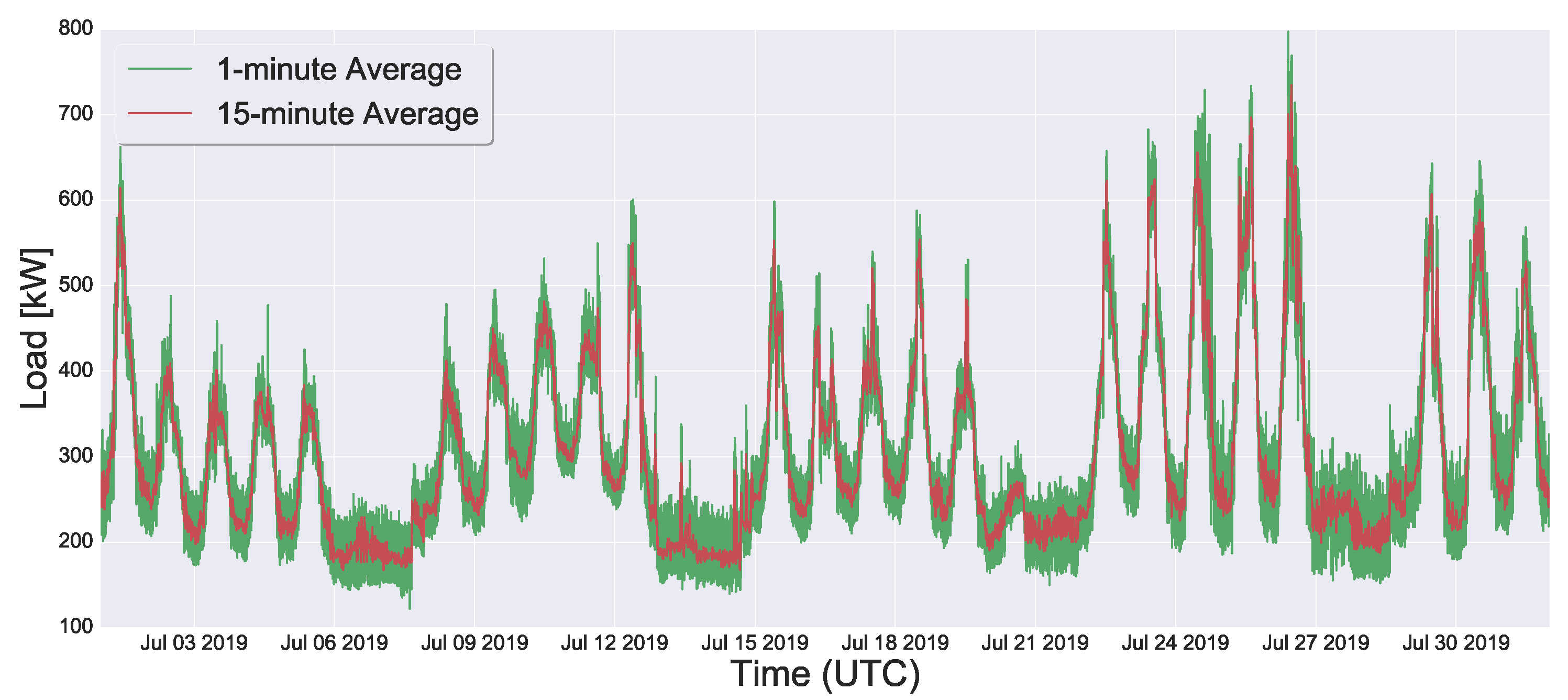
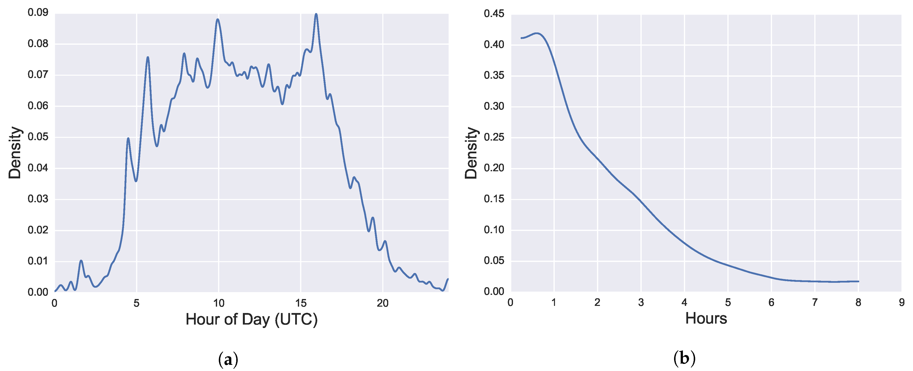
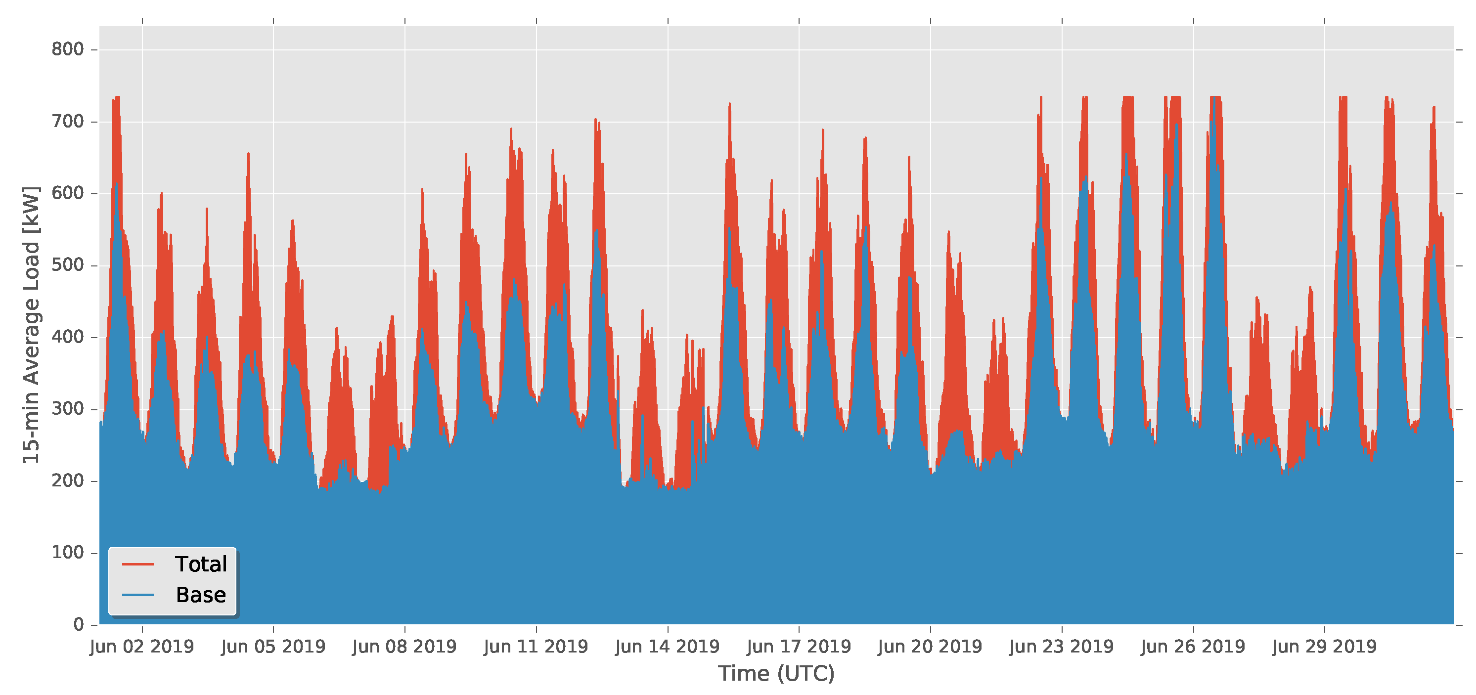
2. Scenario

In simulations, we reflect a possible future scenario at an office building with about 200 employees. Currently, 10 public AC charging stations with a maximum charging power of 11.04 kW each are operated in front of the building. The company has to pay a peak demand charge of 100 euros (A euro is about 1.1 US dollar at the time of writing) per kW of the yearly peak of the 15-min average electrical load, where the 15-min averages are computed for the periods from 0:00 to 0:15, from 00:15 to 00:30, and so on. The load is the sum of the building’s base load and the load resulting from charging at the public charging stations. Thus, a high charging load at an inconvenient time can result in a notable increase of the energy bill. This becomes all the more problematic if the number of public charging stations and their utilization increase in the future. Thus, in the simulations, it is assumed that the charging is controlled in order to avoid the 15-min average load exceeding a prespecified limit $P^{lim}$. Furthermore, it is assumed that as much as possible of the energy requirements of the charging EVs should be fulfilled and that the energy should be distributed to the EVs in a fair way. In order to quantify the fairness, we assume that users have a utility function in the battery charge level at departure as illustrated in Figure 1.

The utility reflects the satisfaction of users gained from the charge level. The form of the used utility function is concave, which is a common assumption [14]. A fair distribution of the available energy should maximize the sum of the utilities of all users, which is the case if EVs with a low charge level are preferred in the distribution of the energy (due to the concave form of the utility function).

In the simulation, D = 31 days are simulated with a resolution $\Delta t$ of 1 s. As base load, the real base load of the office building from July 2019 is assumed. July is one of the months of the year with the highest peaks in the load of the building. The load is available with a resolution of 1 min. Figure 2 shows a plot of the 1-min and 15-min average load.

The peak of the 15-min average load is 734  kW. Thus, the load limit $P^{lim}$ is set to 735  kW in the simulations, if not otherwise stated.

It is assumed that, each simulated day d, a certain number $N^d$ of EVs arrive at the charging stations. From the literature, only little information regarding a realistic setting of the distribution of $N^d$ can be gained. However, assuming a normal distribution appears reasonable. Thus, in the simulations, the number $N^d$ of EVs arriving at day d is drawn from a normal distribution with a certain mean $N_M$ and a standard deviation of 20. It is assumed that arriving EVs immediately leave if all charging stations are already occupied by other EVs. The maximum charging power $P_{CS}^{max}$ of the charging stations is set to 11.04  kW. For each arriving EV n, the maximum charging power $P_n^{max}$ is chosen uniformly distributed between 3.7  kW and 11  kW. The lower and upper bounds for the charging power reflect the charging with one and three phases, respectively, with a current of 16 A. The battery capacity $C_n$ of an EV n is uniformly sampled between 20  kWh and 50  kWh, representing a range from small to medium capacities. The initial charge level $E_n^{init}$ is chosen between $0.1C_n$ and $0.8C_n$. It is assumed that the EVs want to charge as much energy as possible. Hence, the energy requirement $E_n^{req}$ of an EV n is set to

$$E_n^{req}=min(min(P_n^{max},P_{CS}^{max})·S_n,C_n-E_n^{init}),$$

(1)

where $S_n$ is the sojourn time of EV n (i.e., the time that the EV is plugged in) in hours.

Table 1. Summary of important simulation parameters. Values in brackets denote ranges of uniform distributions.

Parameter	D	$\Delta \mathit{t}$	${\mathit{P}}^{\mathit{lim}}$	${\mathit{N}}^{\mathit{d}}$	${\mathit{P}}_{\mathit{CS}}^{\mathit{max}}$	${\mathit{P}}_{\mathit{n}}^{\mathit{max}}$	${\mathit{C}}_{\mathit{n}}$	${\mathit{E}}_{\mathit{n}}^{\mathit{init}}$
Unit	-	s	kW	-	kW	kW	kWh	kWh
Value	31	1	735	$\mathcal{N}(N_M,{20}^2)$	11.04	$[3.7,11]$	$[20,50]$	$[0.1,0.8]·C_n$

summarizes the important parameters of the simulation.

The arrival and sojourn times of the EVs are generated based on real data of public charging sessions in the United States (The data is Honda internal, and we cannot provide full information on it due to confidentiality). Kernel density estimations are fitted to the data in order to derive corresponding probability distributions, which are shown in Figure 3. These distributions are used to generate random arrival and sojourn times in the simulations.

In order to evaluate controllers on forecasts of the base load, the load shown in Figure 2 is forecasted with a resolution of 5 min. Each forecast is made for 24 h ahead (i.e., 288 5-min average load values are forecasted in each forecast). Since forecasts for time steps near in the future are usually more accurate than forecasts for time steps farther in the future, the forecasts are updated every 5 min. That means, for all 5-min intervals of the considered time frame of 31 days, a new 24-h ahead forecast is created. The following 37 values are used as inputs for a forecast:

• The 30 previous 5-min average load values
• The index $i\in \{0,\dots ,287\}$ of the first time step to predict within the corresponding day
• The index of the weekday of the first time step to predict, from 0 to 6 or 7 if the day is a national holiday
• The index of the weekday of the last time step to predict, or 7 if the day is a national holiday
• The 5 previous 5-min average wetbulb temperature values

The electrical load from January 2019 to June 2019 is used as training data for the data-driven forecast of the load. The employed machine learning model is not chosen manually, but instead, TPOT (Tree-based Pipeline Optimization Tool) [15,16] is used for this task. TPOT optimizes machine learning pipelines with the help of genetic programming. It selects the steps (data preprocessing method(s) and machine learning model(s)) of the pipeline together with their hyperparameters. TPOT represents machine learning pipelines in form of trees, which makes it very flexible in the pipeline structures it can generate. For example, the results of two different data preprocessing steps could be used as input for a learner whose output could be used as input for another learner. Wang et al. [17] showed that TPOT is highly competitive with manually tuned models for the application of electrical load forecasting. We ran an optimization with TPOT in order to evolve a machine learning pipeline for the described load prediction task. In the optimization, TPOT evaluates pipelines by training them on 90% of the training data and by validating them regarding the mean absolute error on the remaining 10%. Pipepine steps can be selected from 14 data preprocessing methods (e.g., standard scaler and principal component analysis) and from 6 multi-output learners (e.g., random forest and XGBoost). For the load forecasting, we use the pipeline resulting from the optimization with TPOT. The pipeline consists of multiple preprocessing steps and an extra-trees regressor. Figure 4 shows a plot of forecasts, which were generated without updates (meaning that only at the beginning of a new day, a new 24-h-ahead forecast is made).

The prediction errors resulting from the forecasts with updates are listed in

Table 2. Prediction errors of the forecasts of the base load.

Mean Absolute Error (kW)	Mean Percentage Error (%)	Root-Mean-Square Error (kW)
36.6	11.8	50.4

.

The mean percentage error is around 12%. Thus, the accuracy of the forecasts is not very high. The problem is that the irregular and steep peaks in the load cannot be predicted from the available information. Although it might be possible to achieve a slightly better accuracy with other forecasting approaches than the used one, we assume that it is not possible to generate significantly better forecasts than the ones we use in the simulation.

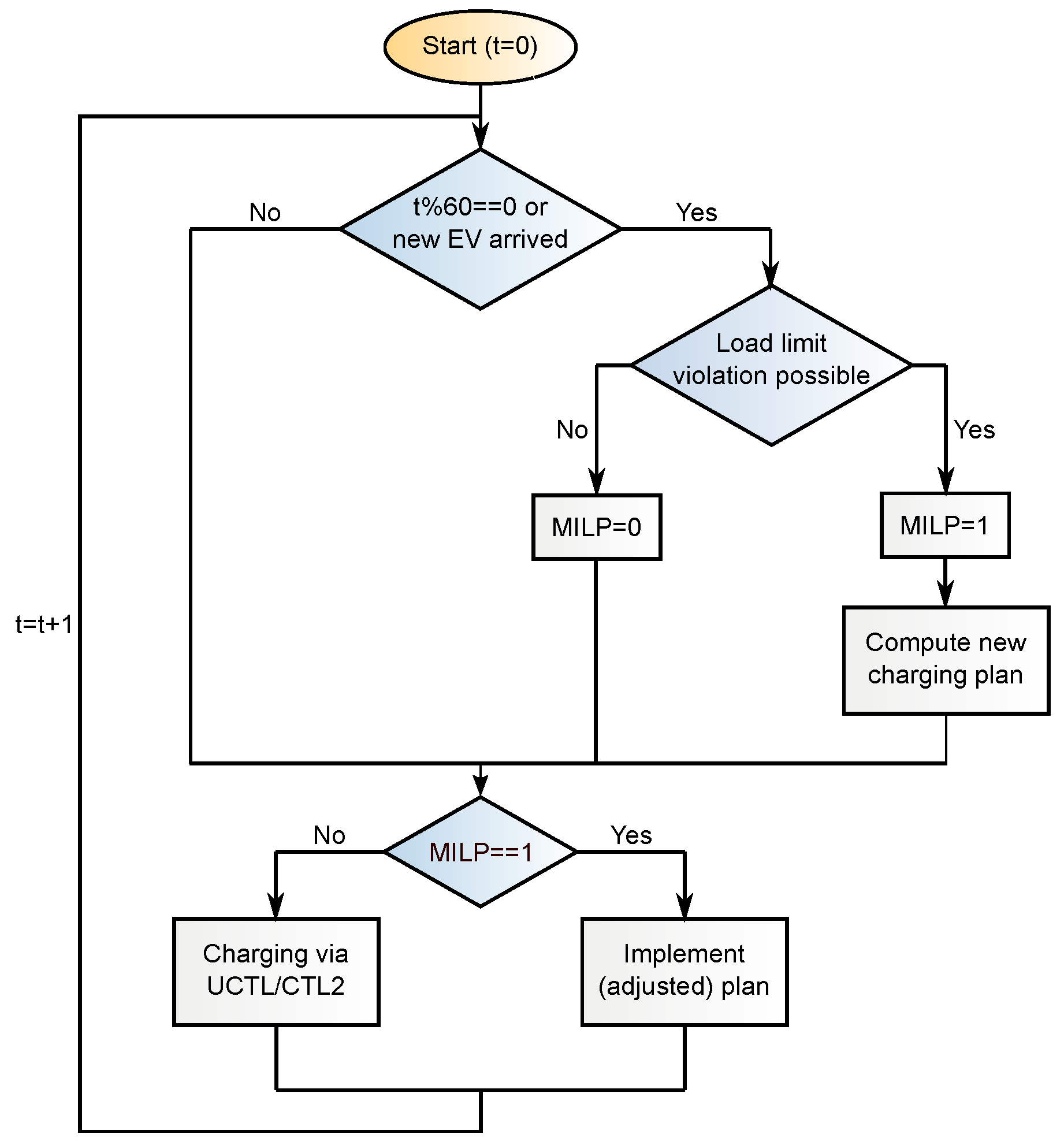
3. Controllers

We compare three control approaches with uncontrolled charging (UCTL), which charges plugged-in EVs until they are fully charged or until they depart: Rule-based control, control based on mixed integer linear programming, and control based on mixed integer quadratic programming.

3.1. Rule-Based Control

The rule-based controller computes every minute a new upper bound for the total charging power based on the energy consumed so far in the current 15-min interval. It assumes that the base load in the following time steps will be the same as the average base load in the last minute. The upper limit for the charging load is computed as

$$P_{charge}^{lim}=max(0,\frac{E_{charge}^{lim}}{T_{remain}·\Delta t}),$$

(2)

where $\Delta t$ is the length of a time step in hours (1/3600 in our case), $T_{remain}$ is the number of time steps remaining in the current 15-min interval, and $E_{charge}^{lim}$ is the energy, which is expected to be consumable in the remaining time steps of the current 15-min interval and which is computed as

$$E_{charge}^{lim}=E_{grid}^{lim}-E_{grid}-T_{remain}·P_{base}^{-1}·\Delta t.$$

(3)

where $E_{grid}^{lim}$ is the total energy, which can be consumed in 15 min ($P^{lim}·15/60$); $E_{grid}$ is the energy, which was consumed so far in the current 15-min interval; and $P_{base}^{-1}$ is the average base load in the previous minute.

In each time step, the allowed charging power is distributed to the plugged-in EVs. We assume two versions of the rule-based controller: The first version, CTL1, distributes the power equally to the EVs. For each EV n, the charging power is set to $P_{charge}^{lim}/N$, with N being the number of currently plugged in EVs. The second version, CTL2, considers the maximum possible charging power of the EVs in the distribution of the charging power, as outlined in Algorithm 1.

Algorithm 1: Distribution of allowed charging power $P_{charge}^{lim}$ to N plugged-in EVs according CTL2

Data: Charging power limit $P_{charge}^{lim}$,     Number N of plugged in EVs,     maximum charging power $P_n^{max}$, battery capacity $C_n$ and charge level $E_n$ of all plugged in EVs n     Result: Charging powers $P_n$ for all plugged in EVs n

First, a charging power $P_{EV}^{lim}$ for each EV is computed analogous to CTL1, then charging powers are allocated to EVs, which are not able to charge with $P_{EV}^{lim}$ because they are (nearly) fully charged or their maximum charging power is too low, and then $P_{EV}^{lim}$ is updated. At the end, the charging powers of remaining EVs are set to $P_{EV}^{lim}$. Note that, in contrast to CTL1, CTL2 has to know the maximum charging powers, battery capacities, and battery levels of all plugged-in EVs.

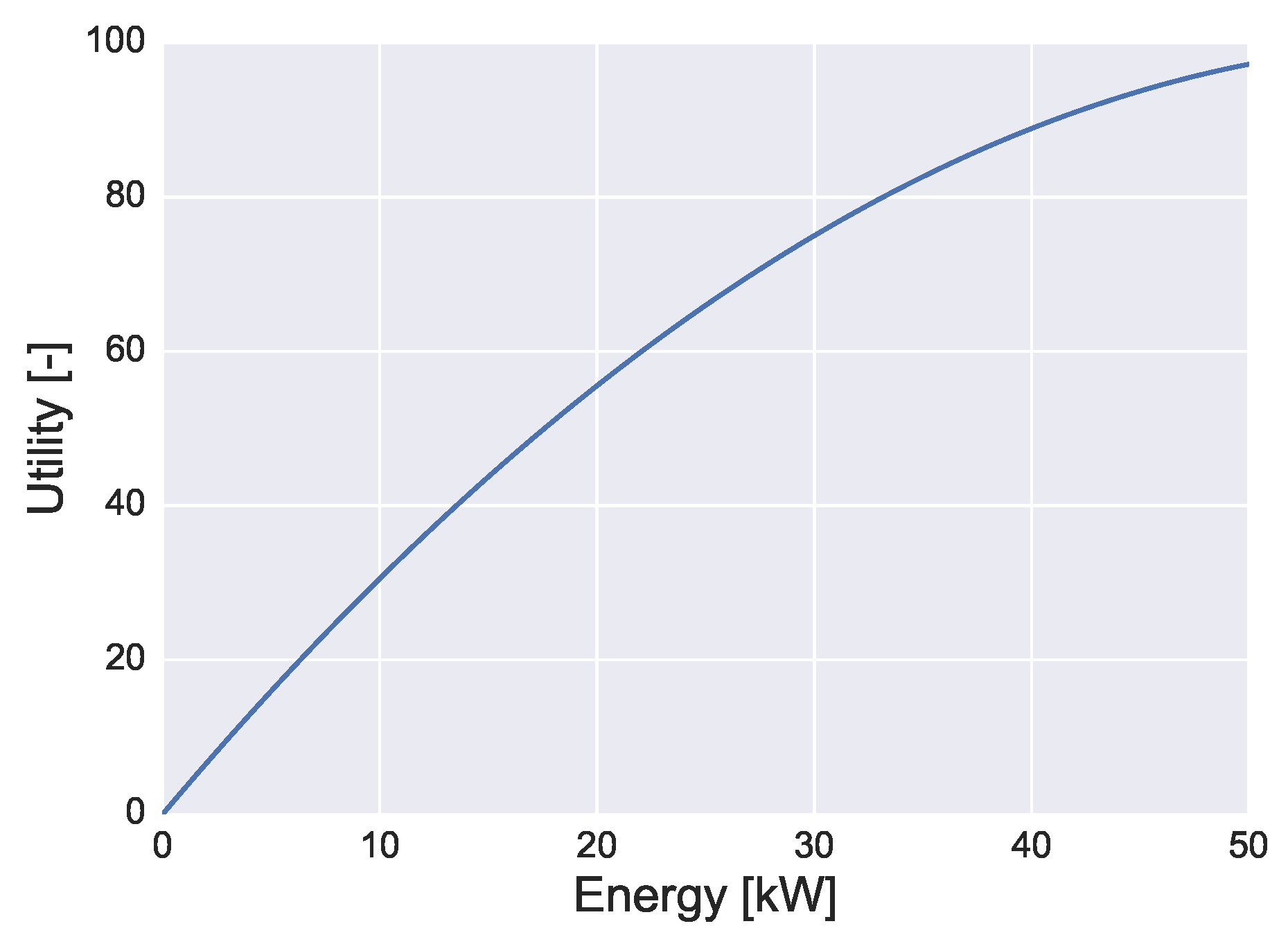
3.2. MILP-Based Control

The MILP-based controller computes charging profiles via MILP. We consider two versions of MILP-based control: An ideal controller ${\mathtt{MILP}}^{\mathtt{true}}$, which works on the true base load values, and a realistic controller ${\mathtt{MILP}}^{\mathtt{pred}}$, which works on predictions of the base load. The workflow of the MILP-based control is outlined in Figure 5.

Every minute and in each time step with a new plugged in EV, it is tested whether a violation of the load limit is possible. More precisely, a charging load profile is computed assuming that all currently plugged-in EVs charge with their respective maximum charging power until they depart. Then, it is checked whether the sum of this charging load profile and the (possibly predicted) base load results in a violation of the load limit. If no violation of the load limit is possible, ${\mathtt{MILP}}^{\mathtt{true}}$ switches the control strategy in the next time steps to uncontrolled charging. ${\mathtt{MILP}}^{\mathtt{pred}}$ switches to the rule-based strategy CTL2 because it cannot fully rely on the predictions of the base load. In the case that a load limit violation is possible, a new charging schedule is computed and is implemented in the next time steps. However, ${\mathtt{MILP}}^{\mathtt{pred}}$ requires a fallback solution to deal with prediction errors. Thus, it sets the charging power of all EVs to zero in time steps for which the rule-based approach sets an upper limit $P_{charge}^{lim}$ of zero for the charging power.

The computation of the charging plan is done with a scheduling interval length of up to 15 min. It requires the knowledge of the departure times and energy requirements of the plugged-in EVs. The plan is computed for all intervals from the current point in time up to the interval in which the last of the currently plugged in EVs departs. In order to be able to keep the 15-min average peak under a certain limit, the scheduling intervals have to be aligned to the 15-min intervals of the day. That is why the length $\Delta s_1$ of the first scheduling interval is set to the time remaining in the current 15-min interval, while the length $\Delta s$ of the following intervals is set to 15 min. With exception of the first scheduling interval, the real or predicted base load is considered as the base load in the computation of the charging plan. For the first scheduling interval, a limit $P_{charge}^{lim}$ for the charging power is computed analogous to CTL2 (Equations (2) and (3)) based on the energy, which was already consumed in the current 15-min interval. However, the version ${\mathtt{MILP}}^{\mathtt{true}}$ does not assume that the load stays the same as in the previous minute but uses the real future load values in the computation of the charging power limit. In order to consider the computed charging power limit for the first interval in the optimization of the charging plan, the base load $P_1^{base}$ for the first scheduling interval is set to $P^{lim}-P_{charge}^{lim}$. For each plugged in EV n, the scheduling interval $D_n$ in which it departs is computed. Furthermore, in order to consider the fact that EVs can depart at any time in this interval, the fraction $F_n\in (0,1]$ that an EV is plugged in during its departure interval is computed and is used in the computation of the charging schedule. In order to compute a charging plan for N plugged-in EVs over S scheduling intervals, the following MILP is solved:

$$\begin{array}{c}\hfill min100\sum _{n=1}^N{E}_n^{obj}+100\sum _{n=1}^N{E}_n^{surplus}-\sum _{s=1}^S\frac{0.05}{s}{P}_s^{charge}\end{array}$$

(4)

subject to

$$\begin{array}{cc}{P}_s^{charge}=\sum _{n=1}^N{\widehat{P}}_{n,s}\mathrm{with}{\widehat{P}}_{n,s}=\left\{\begin{array}{cc}{P}_{n,s}\hfill & ,\mathrm{if}s<D_n\hfill \\ F_n{P}_{n,s}\hfill & ,\mathrm{if}s=D_n\hfill \\ 0\hfill & ,\mathrm{otherwise}\hfill \end{array}\right.\hfill & \hfill \forall s,\end{array}$$

(5)

$$\begin{array}{cc}{P}_s^{charge}\le max(0,P^{lim}-P_s^{base})\hfill & \hfill \forall s,\end{array}$$

(6)

$$\begin{array}{cc}{E}_n^{bat}=E_n^{init}+P_{n,1}\Delta s_1+\sum _{s=2}^{D_n-1}{P}_{n,s}\Delta s+F_n{P}_{n,D_n}\Delta s\hfill & \hfill \forall n,\end{array}$$

(7)

$$\begin{array}{cc}{E}_n^{obj}\ge 1000-E_n^{req}\hfill & \hfill \forall n,\end{array}$$

(8)

$$\begin{array}{cc}{E}_n^{obj}\ge 1000-E_n^{bat}\hfill & \hfill \forall n,\end{array}$$

(9)

$$\begin{array}{cc}{E}_n^{surplus}\ge E_n^{bat}-E_n^{req}\hfill & \hfill \forall n,\end{array}$$

(10)

$$\begin{array}{cc}{E}_n^{surplus}\ge 0\hfill & \hfill \forall n,\end{array}$$

(11)

$$\begin{array}{cc}0\le P_{n,s}\le min(P_n^{max},P_{CS}^{max})\hfill & \hfill \forall n,\forall s\end{array}$$

(12)

The variable $E_n^{obj}$ reflects how much of the energy requirement $E_n^{req}$ of EV n is unsatisfied. By the constraints of Equations (8) and (9), it is set to $1000-min(E_n^{req},E_n^{bat})$, where $E_n^{bat}$ is the charge level of EV n after charging set by the constraint of Equation (7). The variable $E_n^{surplus}$ is the amount of energy by which the final charge level of EV n exceeds its energy requirement, and it is set by the constraints of Equations (10) and (11). $P_s^{charge}$ is the total charging power in scheduling interval s and is set by the constraint of Equation (5). The coefficients of $P_s^{charge}$ in the objective function decrease with an increasing s. This ensures that the EVs are charged as fast as possible. Equation (6) ensures for all scheduling intervals s that the sum of the charging power $P_s^{charge}$ and of the base load $P_s^{base}$ does not exceed the load limit $P^{lim}$ or that the charging power is set to zero if the base load already exceeds the load limit. Equation (12) ensures that an EV is not charged with a higher power than possible.

Compared to the simple rule-based control, the MILP-based control is more compute-intensive. This can cause issues for the practical application. We assume that a latency of 5 s is tolerable. Hence, in the simulations, we set a time limit of 5 s for solving the described MILP-problem.

3.3. MIQP-Based Control

As mentioned in Section 2, it is assumed that an objective of the charging control is to distribute the available energy in a fair way so that the total utility of the users is maximized. This objective cannot be formulated in linear form. That is why we consider a MIQP-based controller. Again, we consider two versions, ${\mathtt{MIQP}}^{\mathtt{true}}$ and ${\mathtt{MIQP}}^{\mathtt{pred}}$, which work on the true load and the forecasted load, respectively. They work like the corresponding MILP-based versions described in the last section. The only difference is that the variables $E_n^{obj}$ are squared in the objective function. The following objective function is used:

$$min\sum _{n=1}^N\frac{{(E_n^{obj})}^2}{2}+100\sum _{n=1}^N{E}_n^{surplus}-\sum _{s=1}^S\frac{0.05}{s}{P}_s^{charge}.$$

(13)

The first term of the objective function shown in Equation (4) is minimized by fulfilling as much as possible of the EVs’ energy requirements, while the minimization of the first term of the objective function shown in Equation (13) additionally requires to distribute the available energy in a way that prefers EVs with a lower battery level.

The MIQP-based control is even more compute-intensive than the MILP-based control. In the simulations, we also set a time limit of 5 s for the MIQP-based control.

4. Simulation Experiments

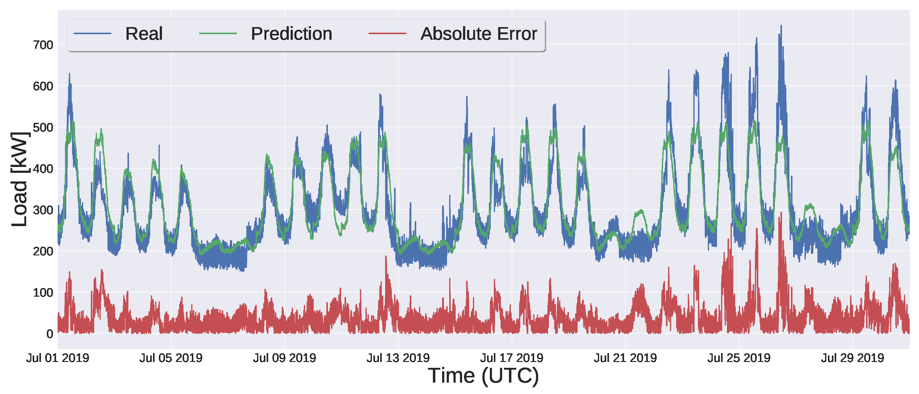
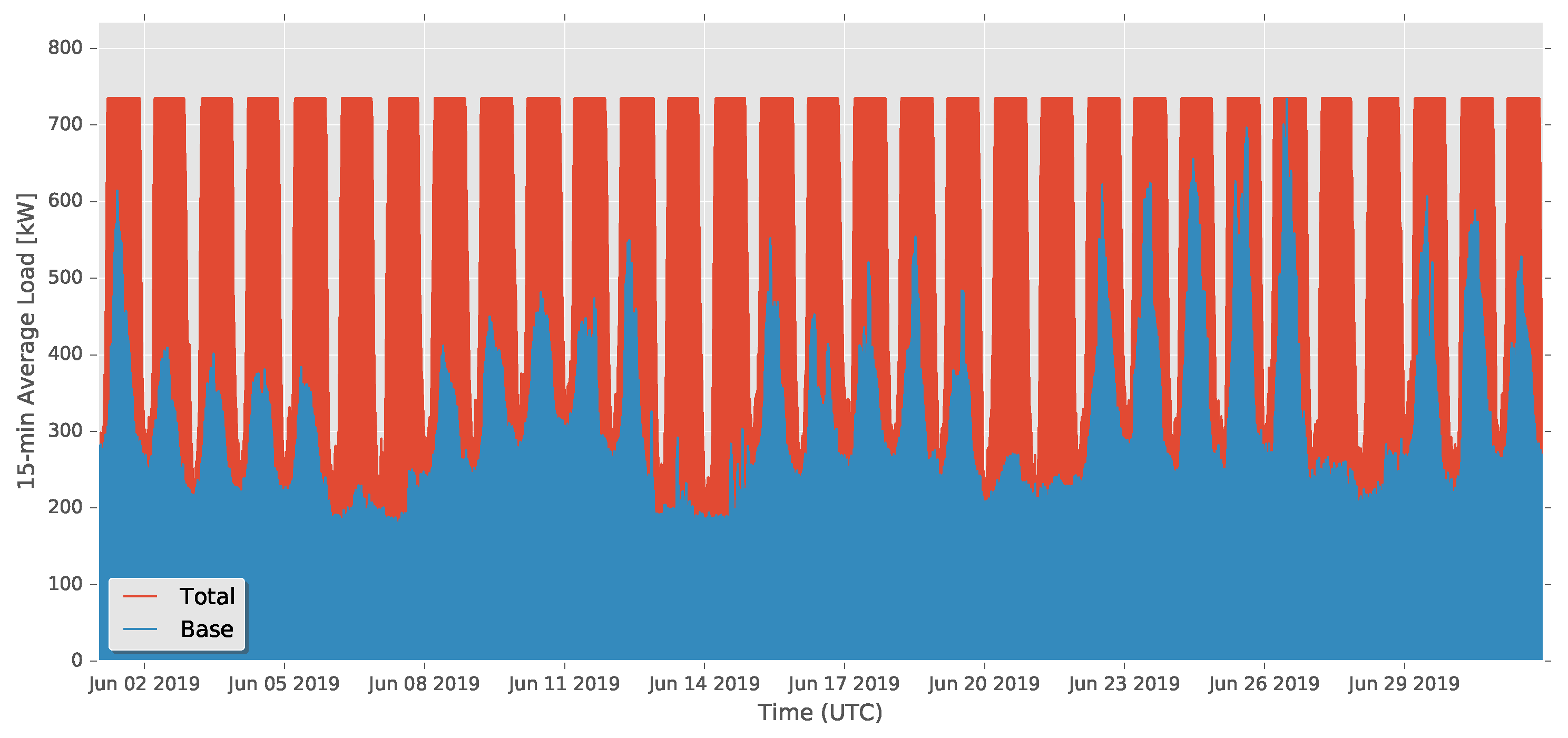
4.1. Experimental Setup

We implemented the simulation of the scenario described in Section 2 with controllers described in Section 3 in C++. Version 5.0.0 of the solver SCIP (Solving Constraint Integer Programs) [18] is used to solve the problems in the MILP- and MIQP-based control. As stated in the previous section, for each problem, a time limit of 5 s is set for its solution. In simulation experiments, we ran the simulation with different mean values $N_M$ of the number of EVs arriving per day and different numbers M of available charging stations. For each setting and each of the considered controllers, we executed 10 trials with 10 different charging requirements (arrival times, energy requirements, etc.) of the EVs on a 3.80  GHz Intel i5-7600 quad-core CPU.

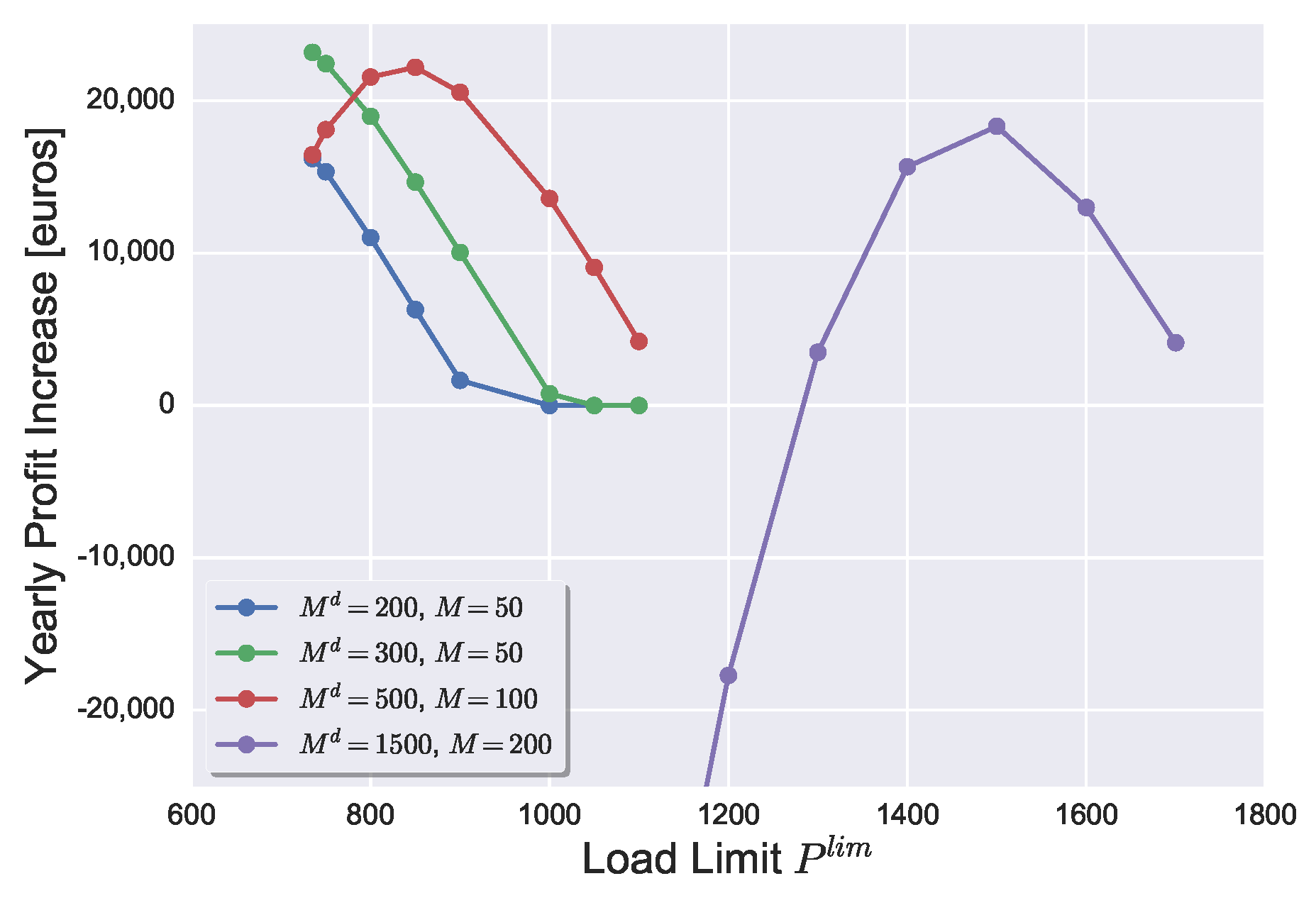
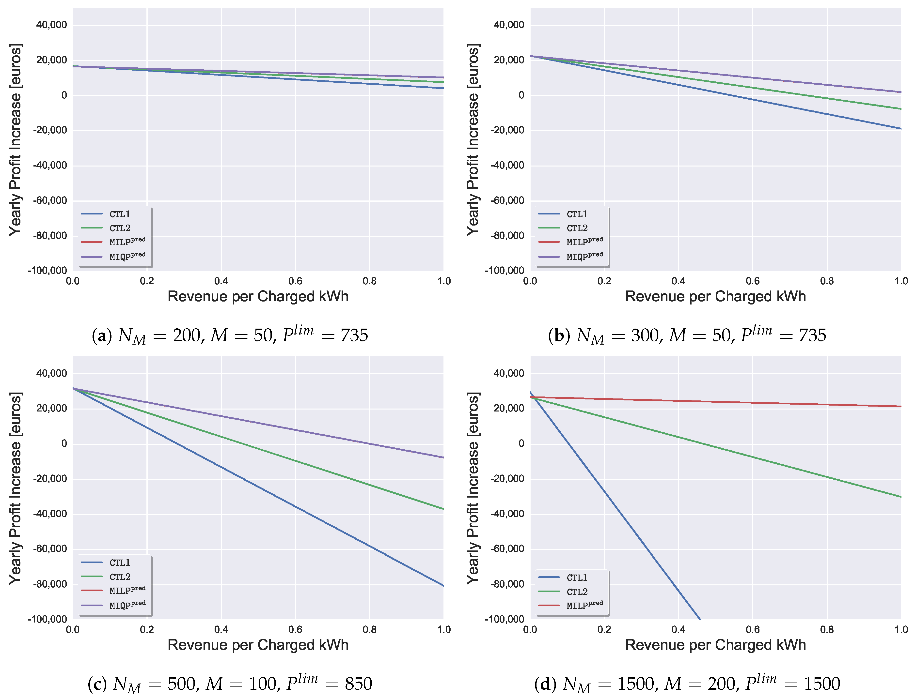
4.2. Experimental Results

In a first experiment, the simulations are done with a mean of $N_M=200$ EVs per day and with $M=50$ available charging stations. With this setup, nearly all arriving EVs can be served. Averaged over the 10 trials, only 2 out of 6136 arriving EVs cannot charge because all charging stations are occupied when they arrive. The results of the simulations with the different control approaches are shown in

Table 3. Results with a mean of $N_M=200$ EVs per day, with $M=50$ charging stations, and with a load limit $P^{lim}$ of 735  kW. Shown are mean values and standard deviations over 10 trials.

	Peak Load (kW)	Unsatisfied Demand (kWh)	Lost Utility per EV
UCTL	$911\pm 28$	$0\pm 0$	$0\pm 0$
CTL1	$742\pm 0.3$	$1054\pm 157$	$0.32\pm 0.05$
CTL2	$743\pm 0$	$754\pm 156$	$0.23\pm 0.05$
${\mathtt{MILP}}^{\mathtt{true}}$	$735\pm 0$	$364\pm 150$	$0.11\pm 0.05$
${\mathtt{MIQP}}^{\mathtt{true}}$	$735\pm 0$	$365\pm 150$	$0.08\pm 0.06$
${\mathtt{MILP}}^{\mathtt{pred}}$	$744\pm 1.0$	$527\pm 137$	$0.16\pm 0.04$
${\mathtt{MIQP}}^{\mathtt{pred}}$	$744\pm 0.7$	$525\pm 138$	$0.14\pm 0.03$

.

Shown are the 15-min average peak loads, the amount of unsatisfied energy requirements of charging EVs, and the amount of utility which is lost per charging EV compared to uncontrolled charging for the seven considered controller variants. More precisely, the mean values and standard deviations over the 10 trials are shown. With uncontrolled charging, the  peak load is on average 911 kW. With the MILP- and MIQP-based controllers on the true load, the peak is exactly at the desired limit. The rule-based control approaches and the optimization-based control on the predicted load result in peaks higher than the limit. However, the exceedance of the load limit can be assumed to be in an acceptable range. It can be seen that CTL2 performs much better than CTL1. This comes at the cost that CTL2 requires more information from the charging EVs than CTL1. With ${\mathtt{MILP}}^{\mathtt{true}}$ and ${\mathtt{MIQP}}^{\mathtt{true}}$, the amount of unsatisfied energy requirements is more than halved compared to CTL2, and with ${\mathtt{MIQP}}^{\mathtt{true}}$, the lost utility per EV is the lowest over all considered controllers. Not surprisingly, the performance of the MILP- and MIQP-based control drops when the control is done only on predictions of the base load. However, the results with ${\mathtt{MILP}}^{\mathtt{pred}}$ and ${\mathtt{MIQP}}^{\mathtt{pred}}$ are still notably better than with CTL2: The amount of unsatisfied energy requirements is on average about 30% lower and the lost utility per charging EV is about 30% to 40% lower. However, the lost utility per charging EV is generally low with all controller versions. The reason is that, most of the time, the EVs can be charged with the maximum possible power, as can be seen from Figure 6, which shows the base load and the total load resulting from ${\mathtt{MILP}}^{\mathtt{true}}$ in the first trial.

There are only a few time periods in which the charging load has to be regulated down in order to not exceed the load limit. Thus, while some of the EVs might lose a high amount of utility due to satisfying the load limit, there is only a small loss of utility seen over all EVs.

In two further experiments, we set $N_M=300$ and $M=50$, and $N_M=500$ and $M=100$. With the first setting, on average, 314 of 9235 arriving EVs leave because all charging stations are occupied, and with the second setting, on average, 9 out of 15,435 arriving EVs leave without charging. The results with $N_M=300$ and $M=50$ are shown in

Table 4. Results with $N_M=300$, $M=50$, and $P^{lim}=735$.

	Peak Load (kW)	Unsatisfied Demand (kWh)	Lost Utility per EV
UCTL	$970\pm 25$	$0\pm 0$	$0\pm 0$
CTL1	$742\pm 0.4$	$3465\pm 150$	$0.73\pm 0.03$
CTL2	$743\pm 0$	$2518\pm 151$	$0.53\pm 0.03$
${\mathtt{MILP}}^{\mathtt{true}}$	$735\pm 0$	$1550\pm 181$	$0.32\pm 0.04$
${\mathtt{MIQP}}^{\mathtt{true}}$	$735\pm 0$	$1549\pm 182$	$0.26\pm 0.04$
${\mathtt{MILP}}^{\mathtt{pred}}$	$744\pm 0.6$	$1712\pm 182$	$0.35\pm 0.04$
${\mathtt{MIQP}}^{\mathtt{pred}}$	$744\pm 1.0$	$1710\pm 180$	$0.30\pm 0.04$

and the results with $N_M=500$ and $M=100$ are shown in

Table 5. Results with $N_M=500$, $M=100$, and $P^{lim}=735$.

	Peak Load (kW)	Unsatisfied Demand (kWh)	Lost Utility per EV
UCTL	$1172\pm 21$	$0\pm 0$	$0\pm 0$
CTL1	$743\pm 0.1$	$\mathrm{23,324}\pm 486$	$2.85\pm 0.06$
CTL2	$743\pm 0$	$\mathrm{19,112}\pm 588$	$2.35\pm 0.07$
${\mathtt{MILP}}^{\mathtt{true}}$	$735\pm 0$	$\mathrm{14,808}\pm 561$	$1.80\pm 0.07$
${\mathtt{MIQP}}^{\mathtt{true}}$	$735\pm 0$	$\mathrm{14,792}\pm 617$	$1.46\pm 0.06$
${\mathtt{MILP}}^{\mathtt{pred}}$	$744\pm 0.8$	$\mathrm{14,905}\pm 555$	$1.79\pm 0.06$
${\mathtt{MIQP}}^{\mathtt{pred}}$	$743\pm 1.1$	$\mathrm{14,900}\pm 556$	$1.47\pm 0.05$

.

Again, all versions of the rule-, MILP, and MIQP-based control are able to satisfy the load limit to an acceptable degree. With the MILP- and MIQP-based controllers working on predictions of the base load, the amount of satisfied energy requirements is increased by around 800 kWh and 4000 kWh, respectively, compared to CTL2. Additionally, the lost utility per charging EV is decreased by 20% to 40%.

In a fourth experiment, we set $N_M=1500$ and $M=200$, resulting in 46,428 EVs which arrive on average, from which 4249 EVs leave without charging because all charging stations are occupied. The simulation results are shown in

Table 6. Results with $N_M=1500$, $M=200$, and $P^{lim}=735$. The problems of the mixed integer quadratic programming (MIQP)-based control could not be solved within the time limit of 5 s.

	Peak Load (kW)	Unsatisfied Demand (kWh)	Lost Utility per EV
UCTL	$1772\pm 17$	$0\pm 0$	$0\pm 0$
CTL1	$743\pm 0$	$\mathrm{241,048}\pm 673$	$11.19\pm 0.03$
CTL2	$743\pm 0$	$\mathrm{239,384}\pm 670$	$11.11\pm 0.03$
${\mathtt{MILP}}^{\mathtt{true}}$	$735\pm 0$	$\mathrm{231,260}\pm 761$	$10.68\pm 0.03$
${\mathtt{MIQP}}^{\mathtt{true}}$	-	-	-
${\mathtt{MILP}}^{\mathtt{pred}}$	$745\pm 2$	$\mathrm{231,319}\pm 756$	$10.62\pm 0.03$
${\mathtt{MIQP}}^{\mathtt{pred}}$	-	-	-

.

With up to 200 EVs which have to be considered in the charging planning, the MIQP problems became too compute-intensive and could not be solved within the time limit of 5 s. Thus, no results for the MIQP-based control are shown. The difference between the peak load with uncontrolled charging and the peak loads with the controlled charging versions would make a difference of more than 100,000 euros in the peak demand charges (assuming 100 euros per kW). However, this comes at the price of more than 200 MW of unsatisfied charging demand. Furthermore, there is a considerable loss of utility per charging EV. Due to the high number of charging EVs, most of the time, the total load is at the limit and the charging has to be regulated down, as can be seen in Figure 7.

The relative difference between CTL2 and ${\mathtt{MILP}}^{\mathtt{pred}}$ is smaller compared to the scenarios with lower numbers of charging EVs. However, ${\mathtt{MILP}}^{\mathtt{pred}}$ still outperforms CTL2 in terms of satisfied charging demand and user utilities.

In all investigated usage scenarios, the rule-based control is outperformed by the optimization-based control, although the optimization-based control is done on base load predictions with a comparatively high error. However, from an economic point of view, there is the question of whether the performance increase justifies the adoption of an optimization-based control, which is more complicated and costly in implementation and operation compared to a rule-based control. More precisely, an optimization-based approach requires a more powerful computational hardware than rule-based approaches. It requires a solver software to solve the optimization problem. A weather forecast might be required in order to predict the base load. Furthermore, an infrastructure is required, which allows users to state their charging requirements. Thus, in the following, it is investigated whether an optimization-based approach is beneficial from an economic point of view. We assume that the charging stations are commercially operated and that the operator gains a certain financial revenue r for each kWh, which is charged. Thus, unsatisfied charging demand results in loss in the revenue. On the other hand, the operator can save peak demand charges by reducing the peak of the 15-min average load. We assume that 100 euros are saved per kW by which the peak is reduced compared to uncontrolled charging as it is in reality for the considered office building. Based on these assumptions, we can compute from the simulation results for each controller version $CTL$ an estimate of the increase of the yearly profit compared to uncontrolled charging as follows:

$$profi{t}^{inc}=100·(pea{k}_{UCTL}-pea{k}_{CTL})-12·r·deman{d}_{CTL}^{uns},$$

(14)

where $pea{k}_{UCTL}$ and $pea{k}_{CTL}$ are the peak loads resulting from uncontrolled charging and controlled charging, respectively, and $deman{d}_{CTL}^{uns}$ is the unsatisfied charging demand resulting from controlled charging according to the simulation results. The unsatisfied demand is multiplied by 12 since, in the simulations, only one month is simulated and we assume that the unsatisfied charging demand is similar in the other months of the year.

From the results in Table 3, Table 4, Table 5 and Table 6 we could now compute the yearly profit increases with different controller versions in the different usage scenarios with Equation (14). However, in the simulations we described so far, we considered a load limit $P^{lim}$ of 735  kW, which might be economically not reasonable—especially for the scenarios with high numbers of charging EVs. Thus, we determined for the different usage scenarios reasonable values for the load limit by simulating one trial (EV charging patterns of the first of the 10 trials are used) with CTL2 control and different values for $P^{lim}$. The corresponding increases of the yearly profit according to Equation (14)) with a revenue r of 0.1 euro per charged kWh are shown in Figure 8.

One can see that, for the scenarios with $M^d=200$ and $M^d=300$, the profit is the highest with a load limit of 735  kW. However, for the scenario with $M^d=500$, a load limit of 850  kW yields the highest profit. For the scenario with $M^d=1500$, the profit is negative for all considered values of the load limit under 1300  kW. The highest profit is achieved with a load limit of 1500  kW. Thus, we repeated the simulations with the rule-based controllers and the optimization-based controllers on the predicted base load for the last two usage scenarios with a load limit of 850  kW and of 1500  kW, respectively. The results are shown in

Table 7. Results over 10 trials for $N_M=500$ and $M=100$, and $N_M=1500$$M=200$ with load limits of 850 kW and 1500 kW, respectively.

$N_M=500$, $M=100$, $P^{lim}=850$ kW
	Peak Load (kW)	Unsatisfied Demand (kWh)	Lost utility per EV
UCTL	$1172\pm 21$	$0\pm 0$	$0\pm 0$
CTL1	$853\pm 0.9$	$9374\pm 280$	$1.12\pm 0.03$
CTL2	$855\pm 0$	$5725\pm 295$	$0.69\pm 0.03$
${\mathtt{MILP}}^{\mathtt{pred}}$	$855\pm 0.02$	$3280\pm 229$	$0.38\pm 0.03$
${\mathtt{MIQP}}^{\mathtt{pred}}$	$855\pm 0.02$	$3279\pm 230$	$0.29\pm 0.02$
$N_M=1500$, $M=200$, $P^{lim}=1500$ kW
UCTL	$1772\pm 17$	$0\pm 0$	$0\pm 0$
CTL1	$1476\pm 3$	$\mathrm{23,553}\pm 282$	$1.01\pm 0.01$
CTL2	$1505\pm 0.3$	$4731\pm 335$	$0.20\pm 0.01$
${\mathtt{MILP}}^{\mathtt{pred}}$	$1504\pm 0.4$	$444\pm 151$	$0.02\pm 0.01$

.

In the scenario with $N_M=1500$, the peak with CTL1 is relatively far below the load limit. The reason is that CTL1 is prone to allocating more power to an EV than the EV is actually able to charge. This results in a high amount of unsatisfied charging demand.

From the mean results in Table 3, Table 4, and Table 7, we computed the corresponding yearly profit increases for different values of the revenue r, between 0 and 1 euro, per charged kWh. The results can be seen in Figure 9. Note that the graphs for ${\mathtt{MILP}}^{\mathtt{pred}}$ are obscured by the graphs for ${\mathtt{MIQP}}^{\mathtt{pred}}$ in the first three plots.

One can see that the difference between the control approaches increases with an increasing number of charging EVs. With a revenue of 1 euro per charged kWh, which can be expected to be unrealistically high (For comparison, the electricity tariff for private households in Germany is on average around 0.3 euro per kWh at the time of writing), the difference between CTL2 and ${\mathtt{MILP}}^{\mathtt{pred}}$ is about 2700 euros in the scenario with $N_M=200$, while in the scenario with $N_M=1500$, the difference in the profit increase is more than 52,000 euros and CTL2 yields a lower profit than uncontrolled charging. With a more realistic revenue of 0.1 euro per kWh, the difference is only about 170 euros in the scenario with $N_M=200$ and about 5200 euros in the scenario with $N_M=1500$. Probably, a yearly profit increase of 170 euros does not justify an adoption of the more complex optimization-based approach while an increase of 5200 euros possibly does. A potential decline of the number of users due to unsatisfied charging demands is not reflected by the computed profit increases. The higher quality of the charging service from a user’s perspective might be an argument for an optimization-based approach, especially for an approach like the MIQP-based approach, which distributes the energy in a fair way.

5. Conclusions

In the present work, optimization-based approaches for EV charging control were compared with rule-based approaches in a realistic scenario based on simulation experiments. The optimization-based approaches outperformed the rule-based approaches, and the MIQP-based approach yielded a higher user utility compared to the MILP-based approach. This is the case not only when the optimization-based approaches work on the real base load but also when they work on a prediction of the base load, although the error of the prediction is comparatively high. However, also the rule-based approaches were able to satisfy the load limit to an acceptable degree. An investigation from an economic point of view has shown that the differences between the results of the optimization-based approaches and those of the rule-based approaches—especially of an advances variant, which considers the current states of the EVs—do not necessarily justify the adoption of optimization-based control, which is more complex and more costly than rule-based control. Furthermore, the MIQP-based approach has the drawback of a high computational intensity. While the MIQP problems could be solved within 5 s for 100 considered EVs, this was no longer the case for 200 EVs. Thus, it can be concluded that it has to be decided based on the concrete scenario which control approach is the most beneficial one. Generally, the optimization-based approaches become more favorable with an increasing number of charging stations and of charging EVs.

Although the used simulation reflects reality to a large degree, it has certain limitations: Delays due to computations and communication are not taken into account. Since the base load was only available with a resolution of 1 min, it is assumed that the rule-based approaches update the charging power limits in intervals of 1 min. For a practical application, a higher update frequency would be preferable and might yield better results. Solving these issues might be a topic of future work.

Furthermore, an analogous comparison of controller approaches for the case of DC fast charging could be an interesting topic of future research. For the case of slow AC charging, which is considered in the present work, the maximum charging power of an EV can be assumed to be independent of its state-of-charge (SOC). This is not the case for DC fast charging, where the maximum charging power considerably reduces with an increasing SOC [19]. The charging profile, which expresses the maximum charging power as a function of the SOC, is typically nonlinear. This could be considered in an optimization-based control with help of nonlinear programming [20] or by using a piece-wise linearization of the charging profile [21]. However, this further increases the compute intensity of the optimization. Even more problematic is that the charging profile is different for different batteries and that it depends on operating conditions, like the ambient temperature [22]. Thus, the exact charging profile is typically not known at the time of charging. A detailed investigation on how this affects the performance of the charging control in practice and how to deal with this issue could be of great value.

A further topic of future work could be the modeling of the reaction of users to unsatisfied charging demands with help of a multi-agent simulation [23] in order to consider potential declines of users due to a low quality of the charging service in the investigation of the economic benefit of different control approaches. Additionally, one could think about extensions of the scenario. A possible extension could be, for example, that different priorities of EVs or of charging points are considered, like it is done by Olson [15].

References

- Chen, N.; Tan, C.W.; Quek, T.Q.S. Electric Vehicle Charging in Smart Grid: Optimality and Valley-Filling Algorithms. IEEE J. Sel. Top. Signal Process. 2014, 8, 1073–1083. [Google Scholar] [CrossRef]
- Zhang, G.; Tan, S.T.; Wang, G.G. Real-Time Smart Charging of Electric Vehicles for Demand Charge Reduction at Non-Residential Sites. IEEE Trans. Smart Grid 2018, 9, 4027–4037. [Google Scholar] [CrossRef]
- Gjelaj, M.; Træholt, C.; Hashemi, S.; Andersen, P.B. Cost-benefit Analysis of a Novel DC Fast-charging Station with a Local Battery Storage for EVs. In Proceedings of the 2017 52nd International Universities Power Engineering Conference (UPEC), Crete, Greece, 28–31 August 2017; pp. 1–6. [Google Scholar] [CrossRef]
- Gjelaj, M.; Træholt, C.; Hashemi, S.; Andersen, P.B. DC Fast-charging Stations for EVs Controlled by a Local Battery Storage in Low Voltage Grids. In Proceedings of the 2017 IEEE Manchester PowerTech, Manchester, UK, 18–22 June 2017; pp. 1–6. [Google Scholar] [CrossRef]
- Wang, Z.; Wang, S. Grid Power Peak Shaving and Valley Filling Using Vehicle-to-Grid Systems. IEEE Trans. Power Deliv. 2013, 28, 1822–1829. [Google Scholar] [CrossRef]
- Alam, M.J.E.; Muttaqi, K.M.; Sutanto, D. A Controllable Local Peak Shaving Strategy for Effective Utilization of PEV Battery Capacity for Distribution Network Support. In Proceedings of the 2014 IEEE Industry Application Society Annual Meeting, Vancouver, BC, Canada, 5–9 October 2014; pp. 1–8. [Google Scholar] [CrossRef]
- Kaur, K.; Dua, A.; Jindal, A.; Kumar, N.; Singh, M.; Vinel, A. A Novel Resource Reservation Scheme for Mobile PHEVs in V2G Environment Using Game Theoretical Approach. IEEE Trans. Veh. Technol. 2015, 64, 5653–5666. [Google Scholar] [CrossRef]
- Gan, L.; Topcu, U.; Low, S.H. Optimal Decentralized Protocol for Electric Vehicle Charging. IEEE Trans. Power Syst. 2013, 28, 940–951. [Google Scholar] [CrossRef]
- Limmer, S.; Rodemann, T. Peak Load Reduction through Dynamic Pricing for Electric Vehicle Charging. Int. J. Electr. Power Energy Syst. 2019, 113, 117–128. [Google Scholar] [CrossRef]
- Flath, C.M.; Ilg, J.P.; Gottwalt, S.; Schmeck, H.; Weinhardt, C. Improving Electric Vehicle Charging Coordination Through Area Pricing. Transp. Sci. 2014, 48, 619–634. [Google Scholar] [CrossRef]
- Huang, J.; Gupta, V.; Huang, Y. Scheduling Algorithms for PHEV Charging in Shared Parking Lots. In Proceedings of the 2012 American Control Conference (ACC), Montreal, QC, Canada, 27–29 June 2012; pp. 276–281. [Google Scholar] [CrossRef]
- Kuran, M.Ş.; Carneiro Viana, A.; Iannone, L.; Kofman, D.; Mermoud, G.; Vasseur, J.P. A Smart Parking Lot Management System for Scheduling the Recharging of Electric Vehicles. IEEE Trans. Smart Grid 2015, 6, 2942–2953. [Google Scholar] [CrossRef]
- Ottesen, S.Ø. Techno-Economic Models in Smart Grids: Demand Side Flexibility Optimization for Bidding and Scheduling Problems. Ph.D. Thesis, Norwegian University of Science and Technology, Trondheim, Norway, 2017. [Google Scholar]
- Limmer, S. Dynamic Pricing for Electric Vehicle Chargin—A Literature Review. Energies 2019, 12, 3574. [Google Scholar] [CrossRef]
- Olson, R.S.; Bartley, N.; Urbanowicz, R.J.; Moore, J.H. Evaluation of a Tree-based Pipeline Optimization Tool for Automating Data Science. In Proceedings of the Genetic and Evolutionary Computation Conference, Denver, CO, USA, 20–24 July 2016; ACM: New York, NY, USA, 2016; pp. 485–492. [Google Scholar] [CrossRef]
- Olson, R.S.; Urbanowicz, R.J.; Andrews, P.C.; Lavender, N.A.; Kidd, L.C.; Moore, J.H. Automating Biomedical Data Science Through Tree-Based Pipeline Optimization. In Proceedings of the 19th European Conference on Applications of Evolutionary Computation, EvoApplications 2016, Porto, Portugal, 30 March–1 April 2016; pp. 123–137. [Google Scholar] [CrossRef]
- Wang, C.; Limmer, S.; Batri, M.; Bäck, T.; Hoos, H.H.; Olhofer, M. Automated Machine Learning for Short-term Electric Load Forecasting. In Proceedings of the 2017 IEEE Symposium Series on Computational Intelligence (SSCI), Honolulu, HI, USA, 27 November–1 December 2017. in press. [Google Scholar]
- Gleixner, A.; Eifler, L.; Gally, T.; Gamrath, G.; Gemander, P.; Gottwald, R.L.; Hendel, G.; Hojny, C.; Koch, T.; Miltenberger, M.; et al. The SCIP Optimization Suite 5.0; Technical Report 17-61, ZIB, Takustr.7; ZIB: Berlin, Germany, 2017. [Google Scholar]
- Dronia, M.; Gallet, M. Field Test of Charging Management System for Electric Vehicle. In Proceedings of the CoFAT 2016—5th Conference on Future Automotive Technology, Fürstenfeld, Austria, 3–4 May 2016. [Google Scholar] [CrossRef]
- Korolko, N.; Sahinoglu, Z. Robust Optimization of EV Charging Schedules in Unregulated Electricity Markets. IEEE Trans. Smart Grid 2017, 8, 149–157. [Google Scholar] [CrossRef]
- Han, J.; Park, J.; Lee, K. Optimal Scheduling for Electric Vehicle Charging under Variable Maximum Charging Power. Energies 2017, 10, 933. [Google Scholar] [CrossRef]
- Mies, J.J.; Helmus, J.R.; Van den Hoed, R. Estimating the Charging Profile of Individual Charge Sessions of Electric Vehicles in The Netherlands. World Electr. Veh. J. 2018, 9, 17. [Google Scholar] [CrossRef]
- Rodemann, T.; Eckhardt, T.; Unger, R.; Schwan, T. Using Agent-Based Customer Modeling for the Evaluation of EV Charging Systems. Energies 2019, 12, 2858. [Google Scholar] [CrossRef]