Article

A Standard-Based Method to Simulate the Behavior of Thermal Solar Systems with a Stratified Storage Tank

by
Edoardo Alessio Piana
1,*,
Benedetta Grassi
2 and
Laurent Socal
3
1
Department of Mechanical and Industrial Engineering, University of Brescia, 25123 Brescia, Italy
2
Independent Consultant, 25128 Brescia, Italy
3
Independent Consultant, 30020 Noventa di Piave, Italy
*
Author to whom correspondence should be addressed.
Energies 2020, 13(1), 266; https://doi.org/10.3390/en13010266
Submission received: 10 December 2019 / Revised: 31 December 2019 / Accepted: 3 January 2020 / Published: 5 January 2020

Abstract

:
Thermal solar systems are interesting solutions to reduce CO 2 emissions and gradually promote the use of renewable sources. However, sizing such systems and analysing their behavior are still challenging issues, especially for the trade-off between useful solar energy maximization and stagnation risk minimization. The new EPB (Energy Performance of Buildings) standard EN 15316-4-3:2017 offers several methods to evaluate the performance of a forced circulation solar system. One of them is a dynamic hourly method that must be used together with EN 15316-5:2017 for the simulation of the stratified storage tank connected with the solar loop. In this work, such dynamic hourly method is extended to provide more realistic predictions. In particular, modeling of the pump operation due to solar fluid temperature exceeding a set threshold, or due to low temperature differential between solar field and storage tank, is introduced as an on–off control. The implemented code is applied to a case study of solar system for the preparation of domestic hot water and the impact of different design parameters is evaluated. The model predicts a higher risk of overtemperature lock-out or stagnation when the solar field surface is increased, the storage volume is reduced and water consumption is set to zero to simulate summer vacation periods. Finally, a simple modulating control with a time step of a few seconds to a few minutes is introduced, quantitatively showing the resulting benefits in terms of useful solar energy increase, back-up operation savings and reduced auxiliary energy use.

Graphical Abstract

1. Introduction

Thermal solar systems are of interest to reduce CO 2 emissions and gradually introduce renewable sources as a replacement for fossil fuels. The sun is indeed one of the main potential sources of energy, with an estimated 120,000 TW of power excluding the radiation reflected by the atmosphere. According to Ivancic et al. [1], this large potential is not fully deployed yet, with a share in heating and cooling applications still below 1%. This may be partly due to the 2008 economic crisis, which hit particularly hard on the works entailing a large initial investment, but also to the existence of several alternatives to increase the energy performance of buildings and fulfill legal obligations [2], to the growth of competing sources, such as photovoltaic, and to the discontinuous availability of solar energy that requires storage capacity. Thermal solar systems coupled with a storage are among the most economically viable renewable energy storage systems to produce domestic hot water enabling, inter alia, the reduction of peak loads associated with water heating. Pezzutto et al. [3] analyze data collected from various sources about the potential in space heating and domestic hot water applications in Europe, showing that the number of installed solar collectors slightly exceeds one million, 85% of which are flat plate collectors, for a total of 1000 annual equivalent full-load hours, about 50% less than combined heat and power internal combustion units.
In a recent review, Gautam et al. [4] summarize the main types, components and technical advancements of solar heating systems, but above all, they stress the importance of increasing the performances in order to build more reliable systems and reduce the payback time. Hernandez and Kenny [5] focus on solar systems for the preparation of domestic hot water. On the one hand, the authors present the most widespread calculation methods, from rule-of-thumb correlations to extremely detailed software simulations and identify the fundamental calculation outputs. On the other hand, they compare the predicted and measured savings of some real installations in Ireland, showing how proper sizing, installation and operation/control have a paramount impact on system performances.
One of the most relevant technical problems to face when dealing with thermal solar systems is stagnation. Stagnation is the condition in which the energy flow absorbed and not transmitted to the connected system is completely wasted as thermal losses by the collector. In forced-circulation solar systems, this condition is triggered when the output temperature of the collector reaches the maximum set and the solar pump is turned off. This determines the overheating of the collector and can even lead to fluid boiling; such a condition is destructive because it may result in materials deterioration and premature aging, deformation of components and degradation of the heat transfer fluid that, becoming more acid, gets extremely corrosive [6,7]. Some interesting experimental data on the evolution of the temperatures in a solar system can be found in [8]. The set-up is located in Spain and the study is performed in April. The water temperature in the top portion of the solar field is reported to grow by 4–6 C per minute, so that in only a quarter of an hour steam bubbles appear in the flow. In this respect, solutions with draining features like the so-called “drain-back” systems are a possible alternative [9] that, however, introduces other types of practical challenges such as loop design to ensure the necessary slope, pump sizing to provide the initial head required to fill the system, and suitability to cold climates.
The stagnation behavior of a thermal solar system depends on the characteristics and the reciprocal influence of the individual parts. Insights into the solar collectors with respect to stagnation are given in Kessentini et al. [10], who numerically and experimentally develop an overheating-proof collector; Eismann [11], who points out that stagnation temperature is overestimated by the widely used correlation developed by Hollands et al. in the 1970s and proposes an alternative method to study these quantities; Hussain and Harrison [12], who numerically and experimentally study the passive air cooling of a flat collector as a possible mean to control stagnation and extend the life of the component; Streicher [13], focusing on the problem of condensate-induced water hammer occurring during stagnation. Studies on the heat transfer fluid date back the late 1980s, with the works by Rossiter [14] and Clifton et al. [15], and with the series of papers by Monticelli et al. [16,17,18] dedicated to corrosion in solar heating systems. Other information on high-temperature deterioration of solar heat transfer fluid (“glycol cracking”) can be found in reports from chemical manufacturers (see for instance [19,20]).
The solar loop, including collectors, heat exchanger (coil) and storage volume must be seen system-wise, since the control strategy and the water storage tank properties have an important role in the overall performances. It has been shown that obtaining and maintaining thermal stratification has a positive effect on the efficiency, as this allows to deliver highest temperature water to the user, whereas water at the lowest temperatures is sent back to the solar collectors, thus increasing their efficiency [21]. The thermal solar stratified storage tank literature and modeling techniques have been extensively reviewed by Fertahi et al. [22]. The stratification of the storage tank has been a popular topic since the late 2000s, with several works reviewing all aspects of thermal stratification including phenomenology, modeling and performance [23,24] or focusing on specific aspects, such as the influence of charge and discharge cycles on stratification [25].
Concerning control, operation of the collector loop pump is usually controlled according to the temperature difference between the solar field output and the bottom of the storage tank where the solar coil is immersed into. Well-established techniques developed in 1970s–1980s, such as on–off (“bang-bang”) or modulating (“differential”) control, are usually implemented in commercial controllers. Refinements of proportional control are proposed in [26], and complex algorithms are more and more commonly found in the literature, for example using optimal control to determine the correct primary flow rates to maximize energy gain, whilst meeting user-defined tank temperatures with minimum energy usage in the secondary loop of the system [27]. Valdiserri [28] includes on–off control in the TRNSYS simulation of solar water heating systems located in seven European cities, analyzing the effect of night switch-offs.
Modeling approaches and techniques cover a wide portion of thermal solar systems literature. The reference works by Klein, Beckman and Duffie [29,30] date back the late 1970s and were the foundations of the popular f-chart method and TRNSYS simulation software. As a matter of fact, being the system based on solar energy, its modeling is transient by nature, as pointed out by Shrivastava et al. [31], who review the major achievements in solar system from a TRNSYS point of view. f-chart was developed using a large number of transient simulations to develop correlations among dimensionless parameters that could be easily calculated from available input data [32]. The f-chart method is still used nowadays as a base for sizing [33], energy performance evaluations [34] and standards [35], but it assumes that the system is correctly sized and operated.
Standards are indeed another resource in terms of solar heating design and energy performance calculation methods, and in particular the set of standards about Energy Performance of Buildings (EPB). The history of EPB standards is described in [36]. The first mandate to produce a comprehensive set of standards for the application of the first EPB directive (EPBD), 2002/91/EC, was given to CEN (European Committee for Standardization) in 2002. The result was a set of forty standards, issued between 2007 and 2008, whose application turned out to be very difficult due to the very variable quality of individual calculation modules and to the lack of coordination between the modules. The European Commission therefore gave a second mandate to CEN to revise all the standards of the first EPB set, and the work started in 2012 (after the 2010/31/EU directive, “EPBD recast”, had been published) with a preliminary phase which lasted over two years. During this phase an expert group of CEN (core team leaders, CTL) designed a modular structure for the standards, defined their contents and established requirements and common features that all standardization documents should have fulfilled (Detailed Technical Rules, CN/TS 16629:2014). Based on these guidelines, all the standards should have included both monthly and hourly time-step calculation methods and default data set to enable their application even in the absence of national data. Moreover, they should have been tested individually and accompanied by a calculation spreadsheet and a technical report with informative content. This long process was deemed essential to create a common modular framework and a set of consistent, “software proof” calculation modules, that could effectively support regulation and that could be the base of energy performance evaluation software.
Between 2014 and 2016, the whole EPB set of standards has been revised [37]. Among these documents, EN 15316-4-3 [35] now provides three methods to calculate the energy performance of thermal solar systems for domestic hot water (DHW) preparation and space heating (SH). Method 1 allows to estimate the energy performance of solar DHW preparation systems, using overall system performance data in conformity with product standards; method 2 (monthly) and method 3 (hourly) are suitable to evaluate the energy performance of DHW, SH and combined systems, using component data declared in conformity with product standards. Method 2 is still based on f-chart and it can be used to estimate the fraction of the required output energy covered by the thermal solar system month by month. Method 3 allows the calculation of the hourly value of heat collected and delivered to the collector loop. When coupled with the calculation of the stratified storage tank described in EN 15316-5 [38], this allows the calculation of all the relevant temperatures of the system on an hourly time step.
The main goal of the EN 15316-4-3 is the energy assessment of a thermal solar system for energy performance calculation purpose, but introducing some enhancements it can be used also as a modeling tool to check the correct sizing of the system and the possible occurrence of undesired events, such as overheating and boiling. The main modification concerns the control of the solar pump: the standard approach implies that, in presence of a non-negligible solar radiation, the pump is always on and the solar fluid circulates at a fixed flow rate, but this does not match the behavior of real systems, where the pump is switched off under certain conditions. At zero flow, no heat is removed from the solar collectors by the heat transfer fluid, and the collectors and the storage tank become two independent systems until the pump restarts. Moreover, nowadays the pump operation is often modulated according to a reference temperature differential.
In this paper the standard dynamic hourly method of EN 15316-4-3 is implemented in Matlab language and integrated with the possibility to take into account stagnation and custom control types. This is done by introducing a module to check if the maximum loop temperature is exceeded and for the calculation of the solar fluid flow rate at the beginning of each time step, according on the specific control type and based on the current system condition. In case of pump lock-out due to high loop temperature, a literature model for exponential variation of the solar field temperature and a simple approach to take into account heat transfer fluid boiling occurrences are added to the standard solution. The goal is to increase the method prediction capabilities while maintaining the reference EPB framework, that was developed to ensure applicability, consistency and reproducibility and that will be—or has already been—included in the energy performance calculation software packages. With these enhancements, the method can be used even at design stage to make decisions and for sizing purposes. A case study serves as a demonstration of the method potential.

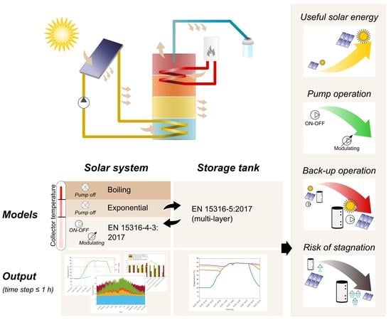
2. Standard-Based Modeling

2.1. Standardized Methods for Thermal Solar Systems

In a thermal solar system, two energy paths can be identified: a primary (generation) solar path starting from the collectors and ending into the storage tank, and a secondary user path (demand), starting in the storage tank and ending at the user terminals (Figure 1). The two paths are considered separately because they run independently, and the storage acts as a connection and buffer between generation and demand. On the generation path, the available solar energy progressively reduces due to thermal solar system losses; on the demand side, the energy must be carried from the storage to the points of use, such as the taps or the heating terminals, thus the energy to be supplied is far more than the needs due to distribution losses. The solar fraction is the ratio between the solar energy that reaches the storage, Q sol ; loop ; out , and the gross need, Q sto ; out , which includes actual needs (for example, Q W ; nd of domestic hot water at the tap) and distribution and storage thermal losses, Q dis ; ls and Q sto ; ls .
Thermal solar systems are nearly always assisted by a back-up heater to supply heat when solar radiation is scarce and/or storage temperature is too low. The solar fraction f sol is the quota of the heat Q sto ; out to be supplied to the distribution system (“load”) which is covered by heat coming from the solar collector, Q sol ; loop ; out . The monthly method described in paragraph 6.1.2 of EN 15316-4-3 is based on the f-chart method, which outputs the solar fraction for each m-th month as
f sol , m = Q sol ; loop ; out , m Q sto ; out , m = a Y m + b X m + c Y m 2 + d X m 2 + e Y m 3 + f X m 3 ,
in which Q sol ; loop ; out , m is the solar contribution in the specific month; Q sto ; out , m is the monthly gross need; X m and Y m are two dimensionless parameters related, respectively, to the collector loop losses and to the solar energy captured by the system, both referred to the total monthly need. The coefficients a f are empirical factors whose values were estimated based on extensive transient simulations [32] and depend on the type of system. The diagram for the use of f-chart method during sizing is shown in Figure 2.
The dynamic hourly method is described in paragraph 6.1.3 of EN 15316-4-3. The calculation is based on an energy balance on the solar collector that, hour by hour, takes into account collected energy, thermal losses and heat removed by the heat transfer fluid. The standard primarily aims to quantify the energy performance of a correctly designed system, and for this reason the method assumes that, as long as the collected energy is significant (at least three times the electric energy consumption of the solar pump), the circulation of fluid never stops and its flow rate is constant in time. This implies that, in this framework, the solar loop and the storage tanks are always interdependent. The calculation flow is shown in Figure 3: after gathering the necessary system information, such as data about the collectors, loop pipes and storage tank, type of application (DHW, SH or combined), set-point temperatures, hourly load and weather data, the calculation is performed for all the time steps h. For each time step, an initial value for average temperature of the collectors θ col ; avg , h is estimated and the corresponding collector efficiency η col , h is calculated as
η col , h = η 0 K hem a 1 T * a 2 T * 2 I sol , h
with
T * = θ col ; avg , h θ e , h I sol , h ,
where η 0 is the zero-loss efficiency of the collector, K hem its incidence angle modifier, a 1 and a 2 the first- and second-order heat loss coefficients (all of which can be found on the collector test report according to EN 12975), θ e the outdoor air temperature and I sol the solar irradiance on the collector plane. The resulting collected heat delivered to the fluid and the solar loop losses are calculated, to obtain the net heat which is transferred to the water stored in the tank. The multi-layer model described in EN 15316-5 standard is then invoked. The temperature of the layer that the solar loop is immersed into is related to the inlet, outlet and average temperatures of the solar coil, that is, of the collector loop. A new θ col ; avg , h can be calculated and the second iteration starts. The prescribed convergence condition is reached after 4 iterations or when the percentage variation of the solar heat delivered to the stored water with respect to the previous iteration falls below 5%. It is worth noting that the method is dynamic, as the condition at h-th time step depends on the condition at h 1 -th time step.

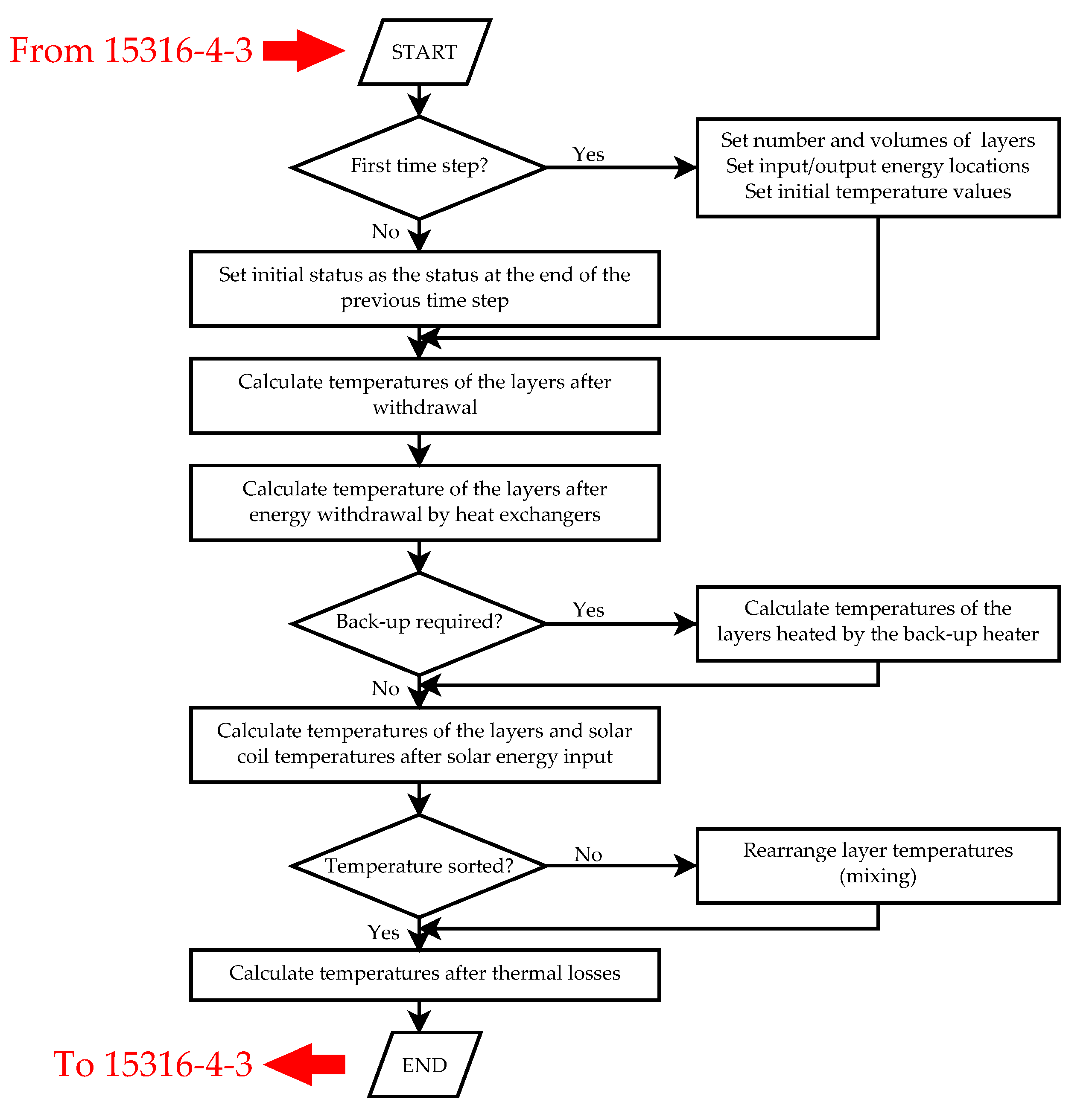
2.2. Standardized Method for Stratified Storage

EN 15316-5 standard allows to calculate the temperature profile of the storage vessel depending on the water draw-off and on the energy supplied to or withdrawn from each layer by heat exchangers. Method A models the storage as a multi-layer unit, whereas Method B as a single-layer unit. Method A is the required option for storage tanks connected to thermal solar systems, where stratification is a key element of solar energy storage and back-up heater contribution minimization. DHW preparation, SH and combined applications can be modeled.
Once the storage volume has been divided into volume layers, initial temperatures are set (for example, set-point temperatures or realistic values for the initial period of calculation). Input and outputs are connected to some of these volume fractions. The default (and minimum) configuration for a storage connected to a thermal solar loop and a back-up heater is a four-layer model, however the number and individual volumes of the layers are a modeling choice. The solar coil is connected to the bottom layer, whereas the back-up coil is usually located in the second-upper layer.
For the purpose of the standard, the energy stored in the tank is estimated (here, energy should be referred to cold water temperature rather than to service temperature as currently specified by the standard). The next step is to calculate the volume withdrawn from the storage in the time step at hand, based on the load profile. In case of DHW service, withdrawals are assumed to occur from the top layer, while an identical amount of cold water enters the bottom of the cylinder (“piston movement”). The resulting temperature profile is obtained as a weighted average on each layer, simulating mixing. The standard already takes into account the effect of the layer temperature on the water volume draw-off as well as the minimum required temperature depending on use.
The possible energy input coming from external sources, such as solar systems and/or back-up generator, are therefore included and the relative temperature increments calculated. If the resulting overall temperature profile is not sorted, it must be rearranged. For this reason, as long as the temperature of layer l is higher than the temperature of the upper layer l + 1 , the two volumes are mixed. Finally, the thermal losses and the inlet/outlet temperatures of the heat exchangers are calculated. Figure 4 shows the flow chart of the calculation procedure. The location of the storage module within the global calculation can be found in Figure 3.

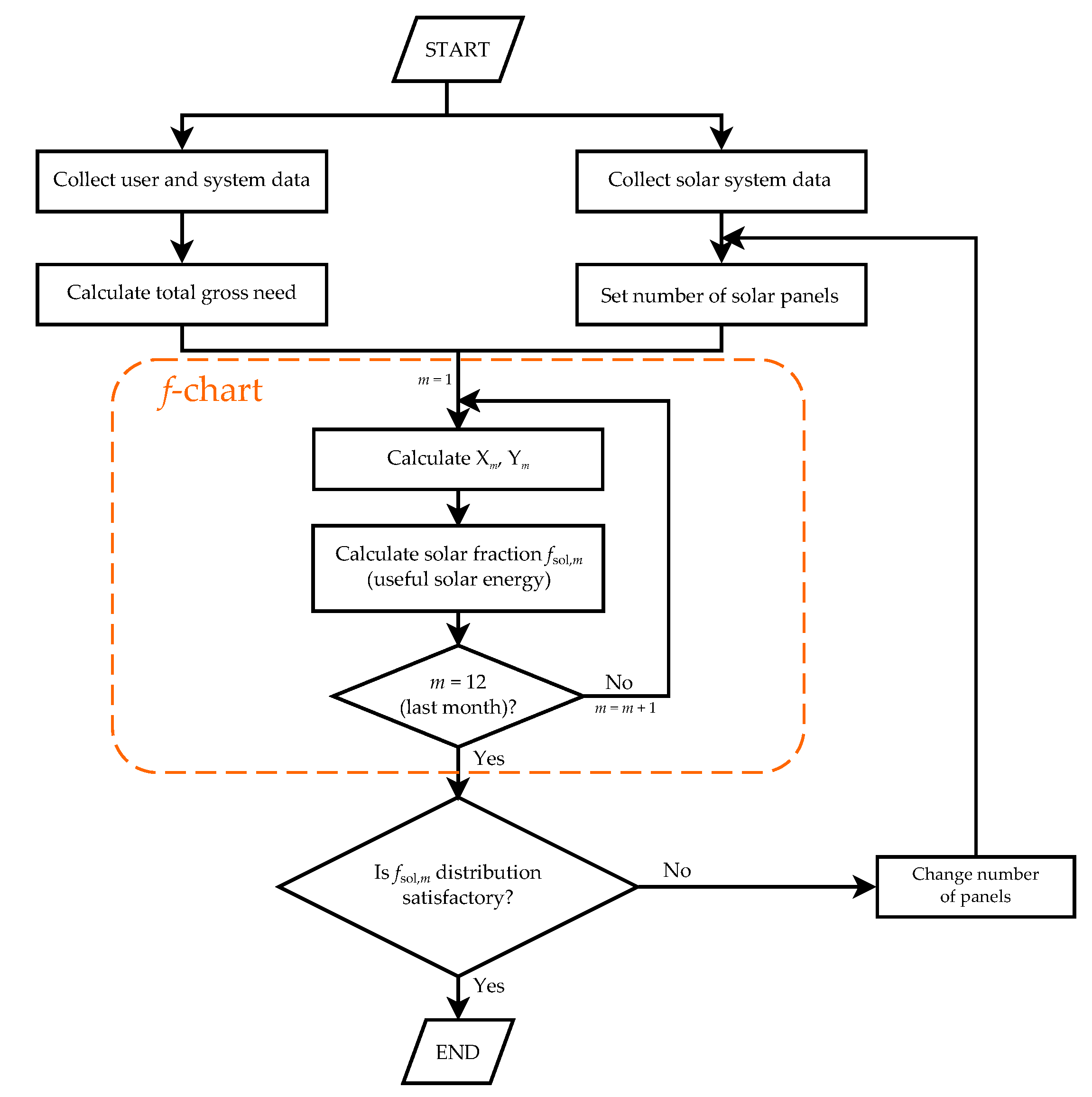
2.3. Modified Dynamic Hourly Method

To expand the capabilities of the standard hourly method, some new aspects must be taken into account:
  • The solar fluid is usually a mixture of glycol and water, not water alone.
  • In a real installation, the thermal solar system is driven by a controller that controls and switches on and off the pump according to the specific conditions
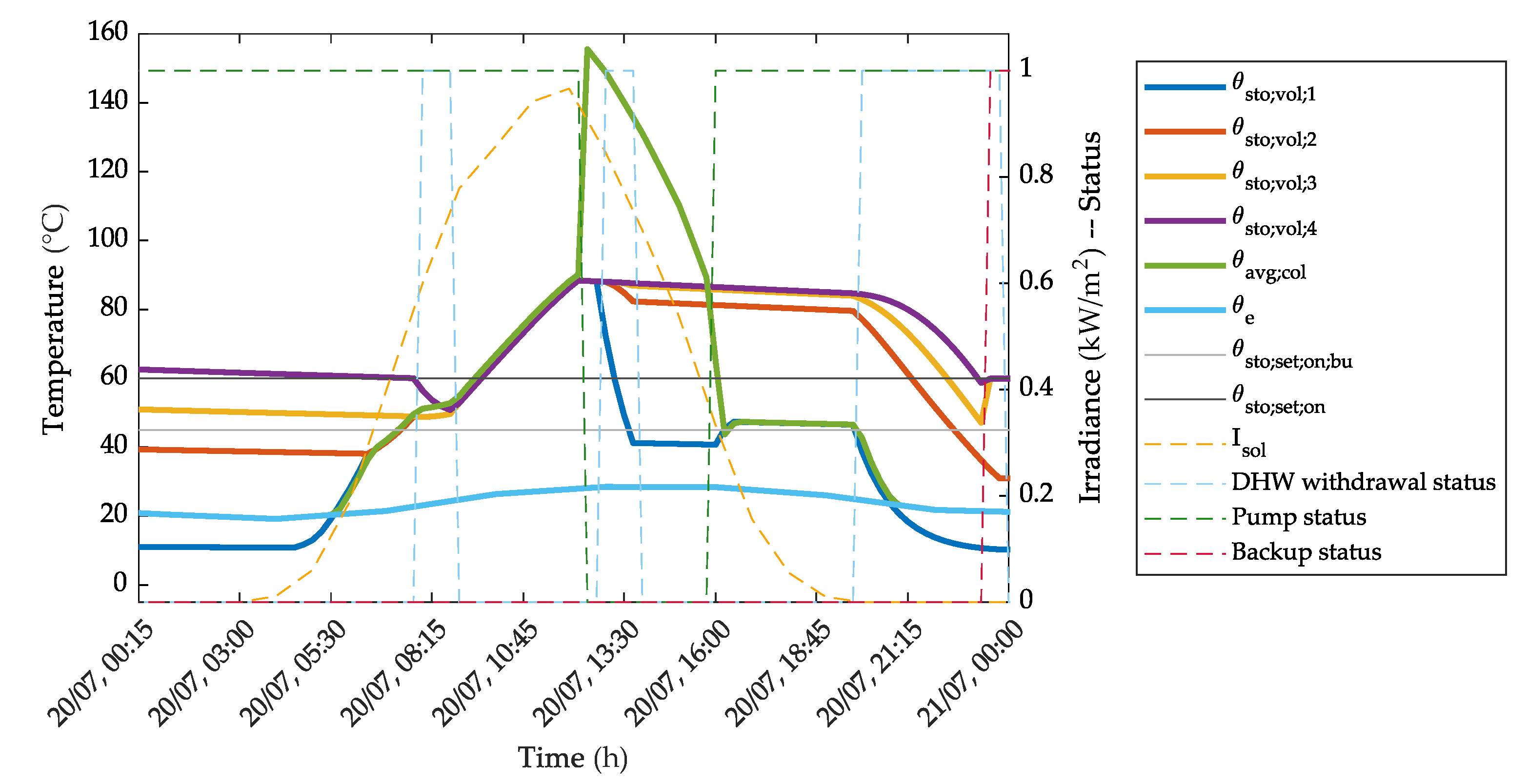
  • When the pump is off, the solar collectors and the storage tank are independent of each other and the average temperature of the collectors depends on the balance between collected solar heat and thermal losses of the collector alone
  • The temperature of the collector may even reach the boiling point. Then the temperature remains constant during the evaporation process and it rises again during superheating, after complete evaporation of the fluid within the collector.
The new elements are incorporated as it follows. First of all, the solar fluid is generally a water-glycol mixture. For the case study presented in this work, a 30% propylene glycol-water mixture has been chosen for its freezing point below −10 C, in the light of the lowest temperatures that can be reached in the considered area. The properties required for the calculation are specific heat at constant pressure c p , density ρ , latent heat of evaporation and boiling temperature. The standard currently recommends to use water properties at 20 C, thus the same temperature is assumed for the mixture properties.
Control-related aspects are taken into account by considering the heat capacity effects and the simplified model by Klein (1974) [32]. In a single-cover collector, whose absorber plate and water content are at uniform temperature T,
m c eff d T d t = Q ˙ sol Q ˙ ls
with ( m c ) eff effective heat capacity of the collector, which can be found on collector test reports according to EN 12975. Q ˙ sol is the flow of solar energy input and Q ˙ ls are the thermal losses. In practical applications, a temperature sensor is mounted on the solar collector outlet, and when its temperature exceeds a safety threshold value the pump is stopped to preserve the loop components. To model this situation, the following assumptions are made:
  • Steady state condition. When the pump is on and the solar fluid flow rate is m ˙ , the standard framework of a steady problem is maintained and the balance on the water-side of the solar collector reads:
    Q ˙ sol = Q ˙ ls = m ˙ c p θ sol ; loop ; out θ sol ; loop ; in
    = 2 × m ˙ c p θ col ; avg θ sol ; loop ; in
    θ col ; avg = Q ˙ sol 2 × m ˙ c p + θ sol ; loop ; in
    which is exactly the equation proposed by the standard (in 2017 version of EN 15316-4-3, in the formula for the calculation of θ col ; avg the solar energy should be divided by the time step to obtain an energy flow).
  • Exponential behavior. When the pump is off due to the solar collector temperature exceeding a safety threshold θ off , the problem can no longer be considered as stationary. Approximating the expression of the captured energy as a first-degree polynomial (that is to say, neglecting a 2 , which leads to underestimate the thermal losses, especially at high temperature), Equation (4) becomes
    m c eff d T d t = A col η 0 K hem I sol A col a 1 T T e ,
    where A col is the reference collector area for η 0 and a 1 . In case a 2 cannot be neglected, a coefficient a = a 1 + a 2 × Δ T could be used in Equation (8) instead of a 1 , with Δ T temperature difference between collector and external air at the previous time step. The differential Equation (8) can be written in the form
    d T d t = K 1 T + K 2
    once the coefficients K 1 and K 2 have been defined:
    K 1 = A col m c eff a 1 K 2 = A col m c eff η 0 K hem I sol + a 1 T e .
    The solution to the differential equation is
    T ( t ) = K 2 + T ( 0 ) K 1 e ( K 1 t ) K 1 K 2 K 1 .
  • Boiling. When the boiling temperature θ boil is reached, the solar input contributes to the evaporation process at constant temperature. This amount of energy must be released completely before the fluid can condense and the temperature can decrease again. A basic model can be introduced in which pressure remains constant during the process, the phase change is uniform in the solar field, and the solar field is at a uniform temperature. When the boiling temperature is achieved the energy balance reads that, in the considered time step of length t ci , the energy available for liquid evaporation is the difference between solar input Q sol and thermal losses Q ls :
    Q sol = I sol A sol K hem η 0 t ci ,
    Q ls = a 1 T * + a 2 T * 2 I sol A sol t ci .
    The total energy contained in the evaporated solar fluid at time step h is
    Q evap , h = Q sol , h Q ls , h + Q evap , h 1 ,
    with Q evap , h 1 energy stored as latent heat during the previous time step, that is to say, in the portion of liquid that has already evaporated. When Q evap , h equals the latent heat of evaporation of the remaining liquid, all the collectors content has evaporated. When Q evap , h becomes zero, the fluid has completely condensed back to liquid. It was chosen to neglect the superheating of the evaporated solar fluid, since the modified method is conceived as a tool to size the plant so to limit the overheating periods as much as possible. In this respect, the sole achievement of boiling periods is a warning that a correction is needed. Moreover, the main time constant of the whole evaporation/recondensation process if often far below the hour.
In conclusion, three cases can be identified which lead to three calculation types (Table 1).
The code has been implemented in Matlab language with the following structure:
  • Input:
    • hourly weather and consumption data
    • system information, including collector, storage and fluid characteristics, and control settings
  • Calculation scripts:
    • main code based on EN 15316-4-3
    • function to check the pertinent case as per Table 1 at each time step
    • code to calculate the fluid flow rate at the beginning of each time step based on the chosen pump control type (standard, on/off with overtemperature lock-out or modulating)
    • storage module, invoked by the main script to provide the stratified storage tank thermal profile and the solar loop inlet and outlet temperatures
  • Output:
    • temperature and status time series for the desired period
    • yearly number of pump operating hours, back-up operating hours and overheating occurrences
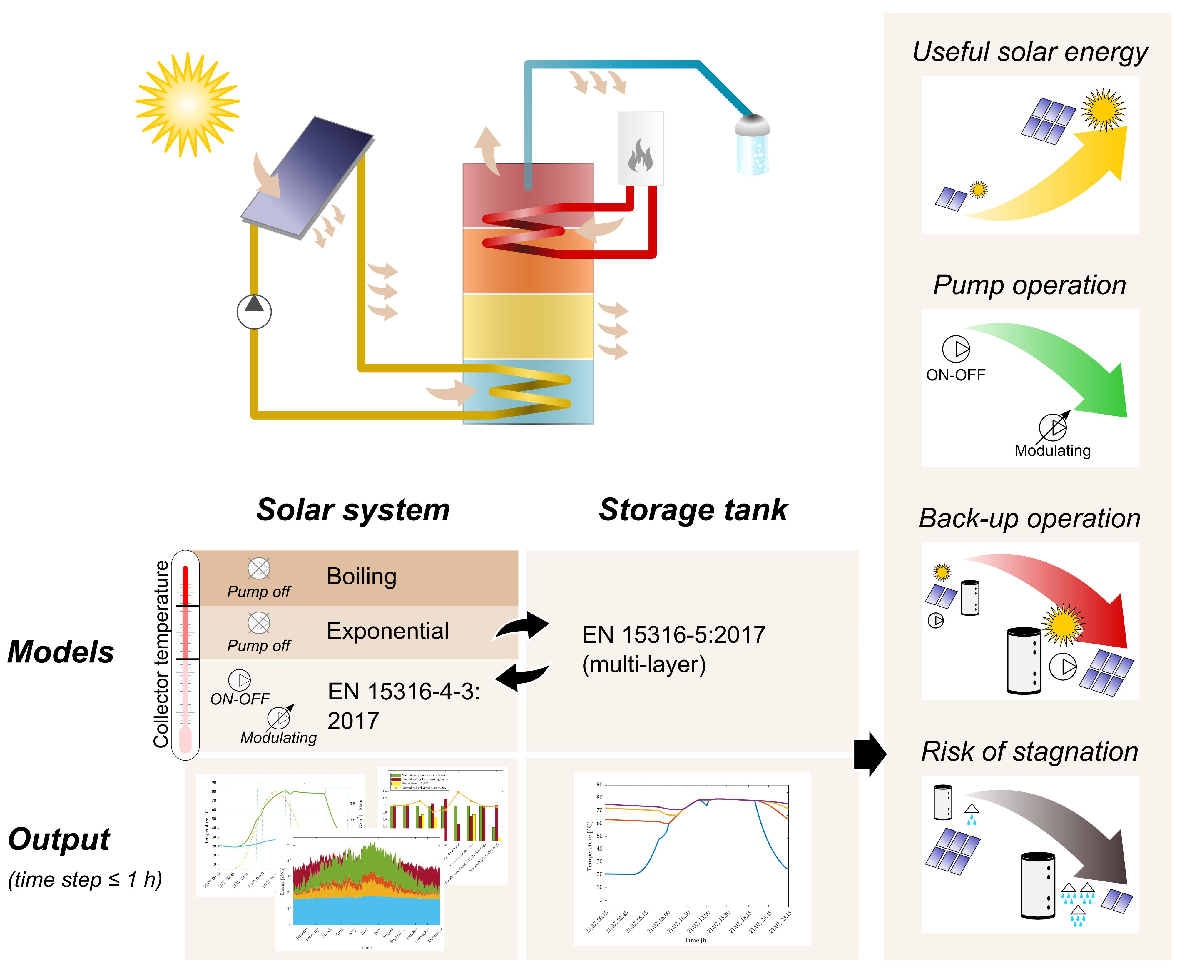
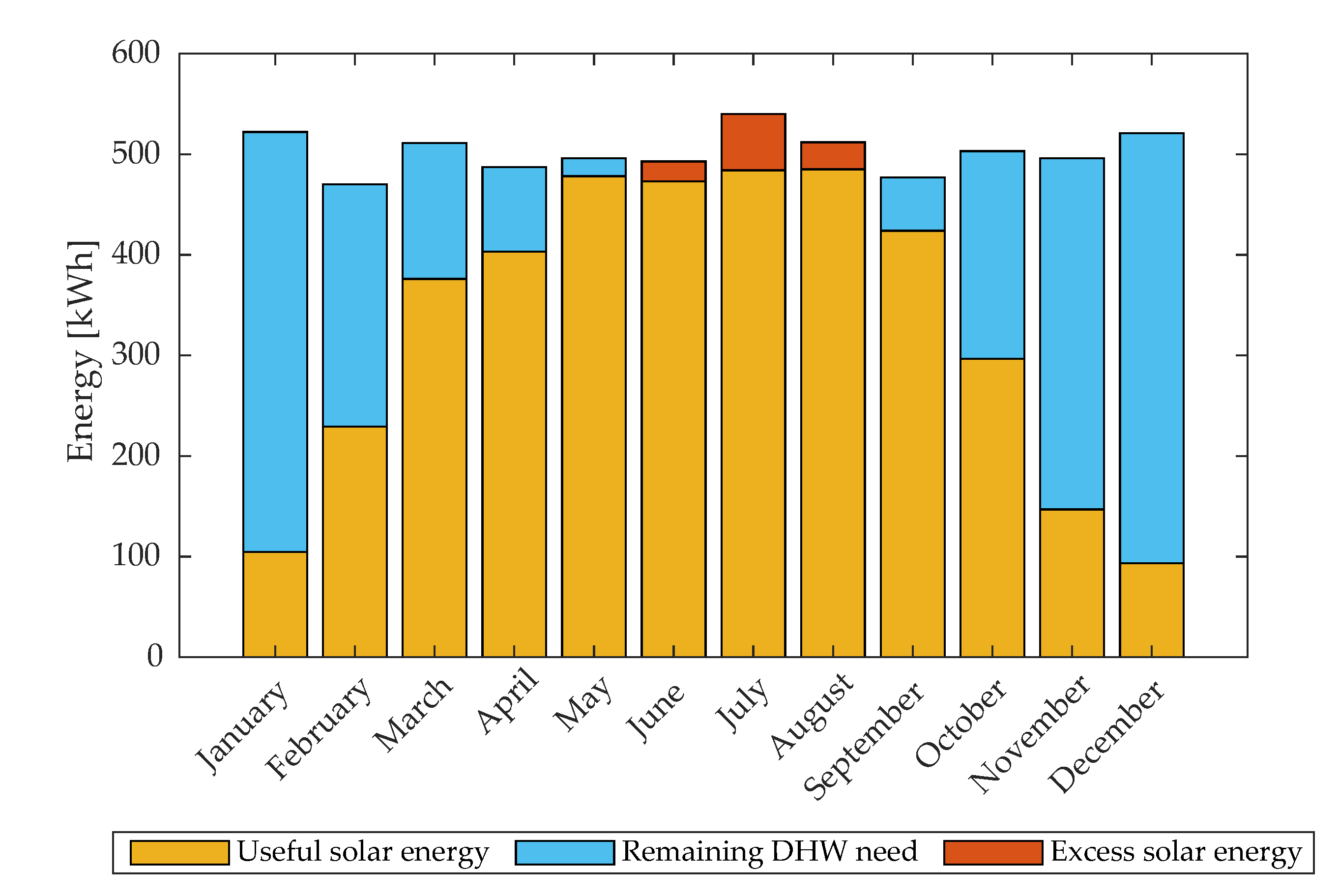
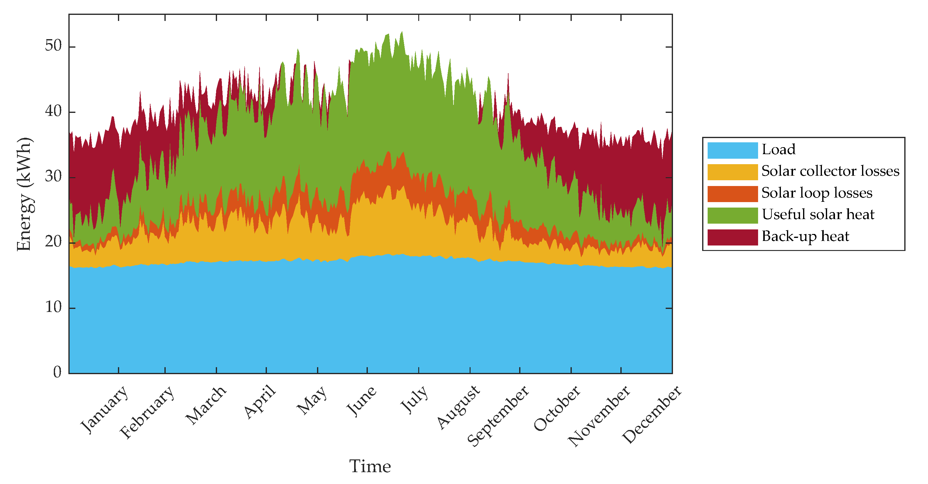
The calculation time for the annual simulation with hourly time step is around 80 s (fourth generation Intel i7 quad-core CPU, 2.50 GHz).

3. A Case Study

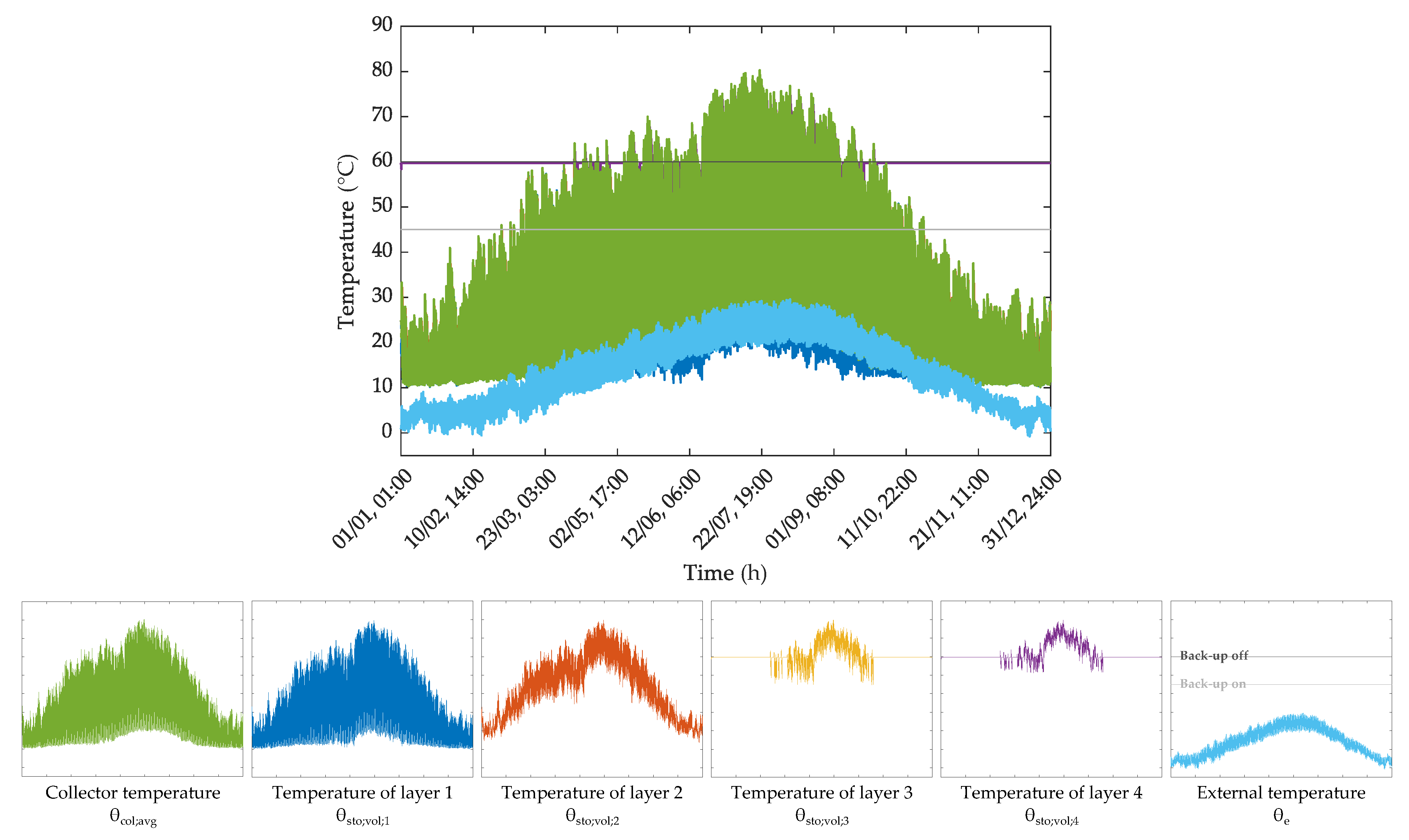
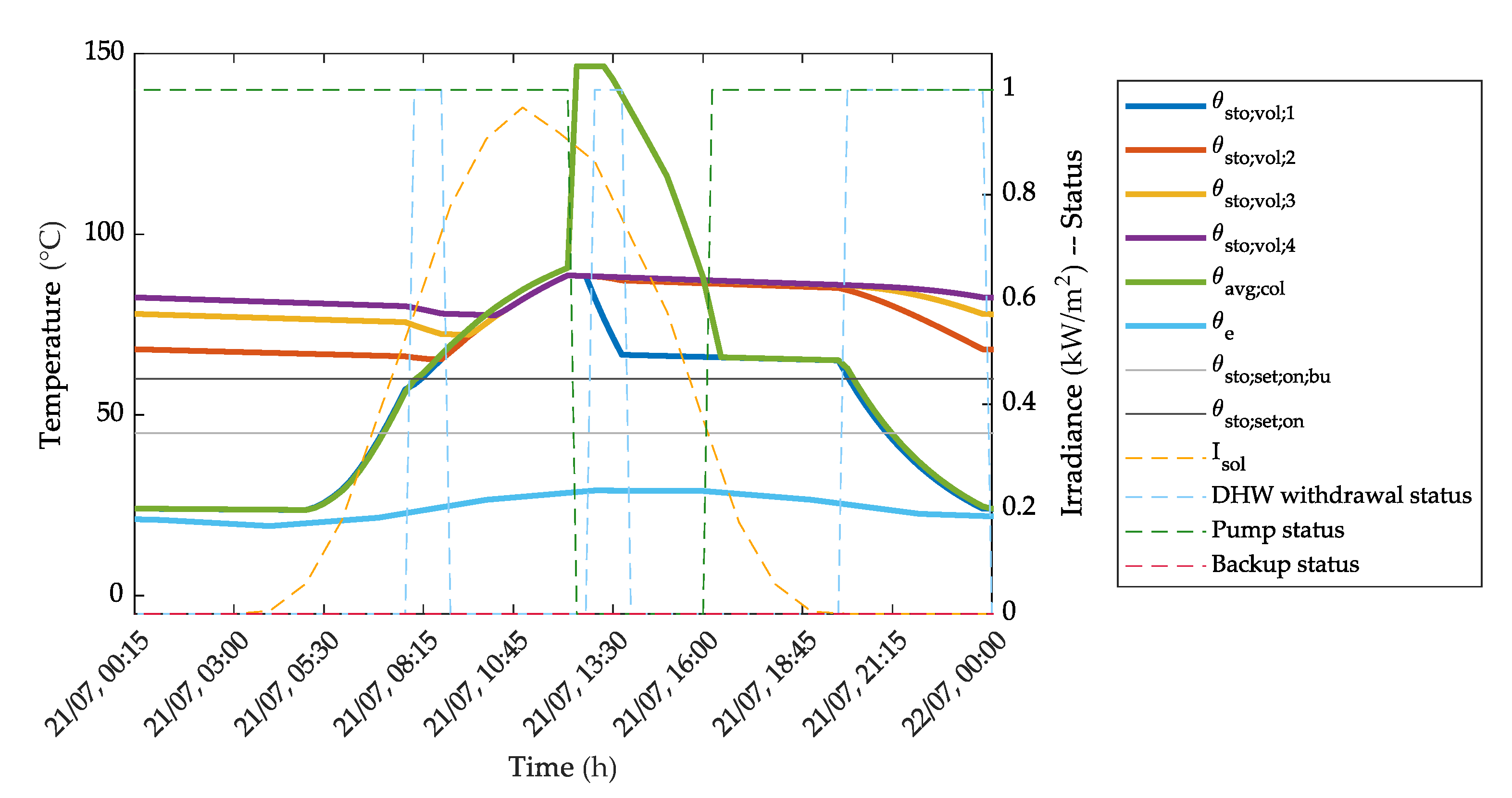
3.1. Preliminary Sizing and Standard Simulations

The goal of the work is to visualize the potential of the hourly method and of its extensions both qualitatively, by means of time series plots, and quantitatively, by means of data analysis. The plots have been extracted for different time intervals: full year, a winter day, a summer day and the transition periods. The simulations also provide the operation time of the solar pump and of the back-up generator, the useful solar energy over the year and the number of times the pump is switched off due to overheating (stagnation cycle). Potentially, all the calculation data can be extracted, processed and displayed.
It was chosen to apply the code to a two-family dwelling in Northern Italy, assuming that the system is used to prepare domestic hot water only. Hourly weather data have been obtained by PVGIS portal [39] as the average of years 2007 to 2016. In case a time step below the hour is set, the code linearly interpolates the available data. The net DHW needs have been estimated based on the Italian standard UNI/TS 11300-2, which, for residential applications, relates the required volume of water at the tap (mixed water, 40 C) to the useful surface of the dwelling. As prescribed by EN 15316-4-3 in the case of unavailability of cold water temperature for the specific location, water mains temperature is assumed as 10 C. The result is approximately 50 L/(person day) for two apartments occupied by 4-people families and, for preliminary sizing purpose, the volume water needs are assumed to be uniform throughout the year. The consumption profile has been set as a typical schedule for a family (six identical 2.32 kWh withdrawals at 8, 13, 20, 21, 22 and 23). The total needs Q sto ; out are obtained as the sum of the net needs and the thermal losses of the domestic hot water distribution and storage subsystems, calculated month by month for the storage tank (volume 500 L) and for the piping system (40 m pipe of internal diameter 16 mm, average distribution temperature 48 C) in three daily hot water tapping cycles, according to EN 15316-3-2 standard.
The heat transfer fluid flow rate has been estimated so that it can remove heat from the collectors at the maximum solar irradiance, with a temperature difference between collector inlet and outlet not exceeding 10 K. After a first sizing stage performed with the monthly f-chart-based method (Figure 5, Table 2), the number of collectors has been set to 4.
The dynamic hourly simulation according to the EN 15316-4-3 standard method has been performed on this demonstrative system. The storage tank has been, for the scope of EN 15316-5 calculations, divided in 4 layers of, respectively, 1/6, 1/2, 1/6 and 1/6 of the total volume from bottom to top. In normal operation, all day long, the back-up generator switches on when the calculated temperature of layer 3 falls below θ sto ; set ; on ; bu = 45 C, and it switches off when the temperatures of layers 3 and 4 reach θ sto ; set ; on = 60 C.
Figure 6 and Figure 7 show the results of the simulation. The time step is 15 min for daily simulations and 1 h elsewhere. From one-day details it can be observed that sun path is regularly followed by the average temperature of the collectors and, as a consequence, by the bottom temperature of the cylinder. As indicated by literature studies [40] the most pronounced thermal stratification occurs in correspondence of consumption periods and over night, whereas during loading the temperature tends to become uniform. The effect of water withdrawals is also observed. Figure 8 shows the distribution of the main input and output energy flows along the year: the back-up heater is on 60% of the time, between late September and mid-April, which is in line with the heating season defined by the Italian legislation for the climatic zone at hand (Presidential Decree 412 of 26 August 1993, zone E, 15 October to 15 April). The overall solar energy delivered to the tank is about 4200 kWh/y. The maximum temperature reached by the solar field is 80 C.

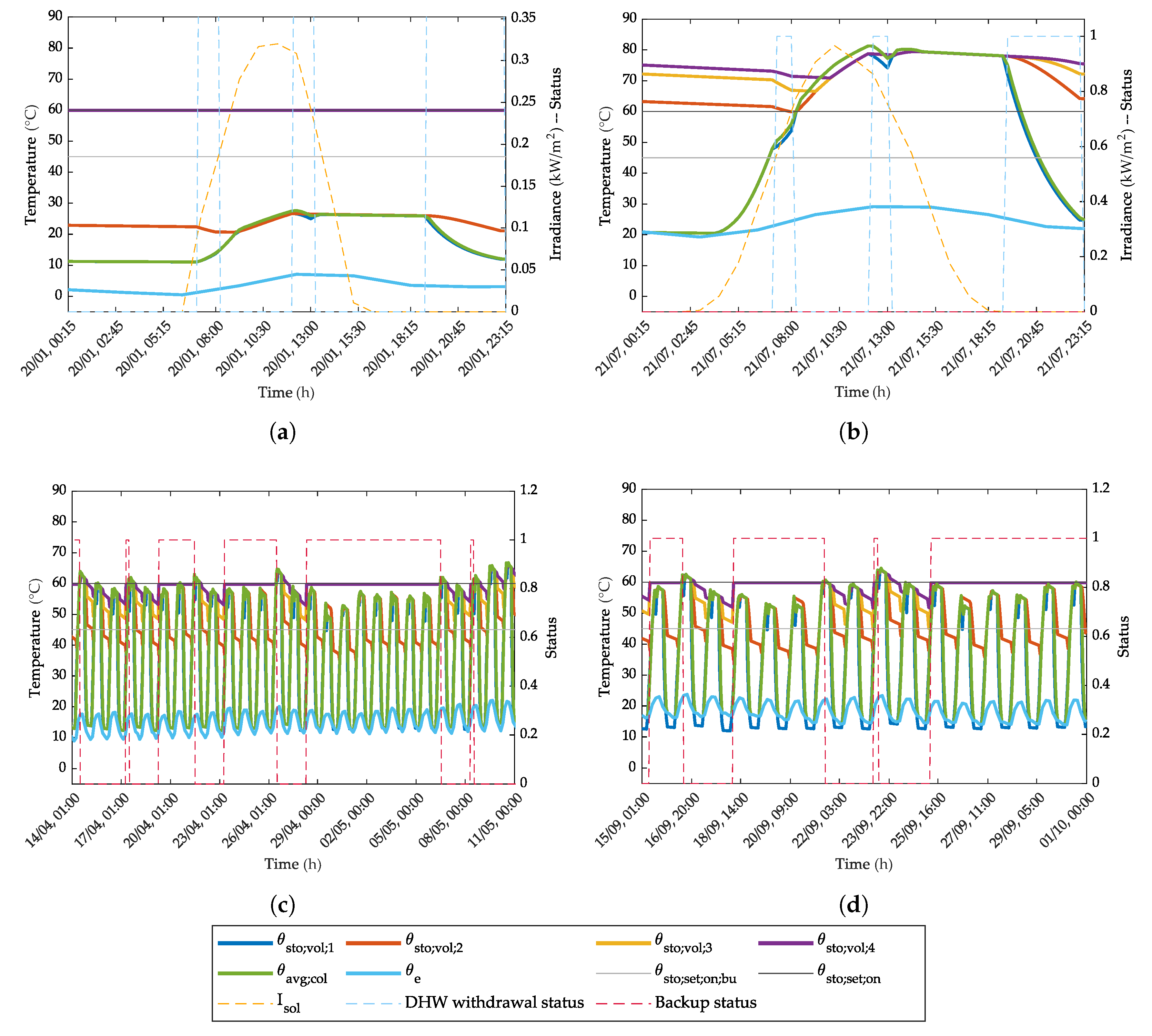
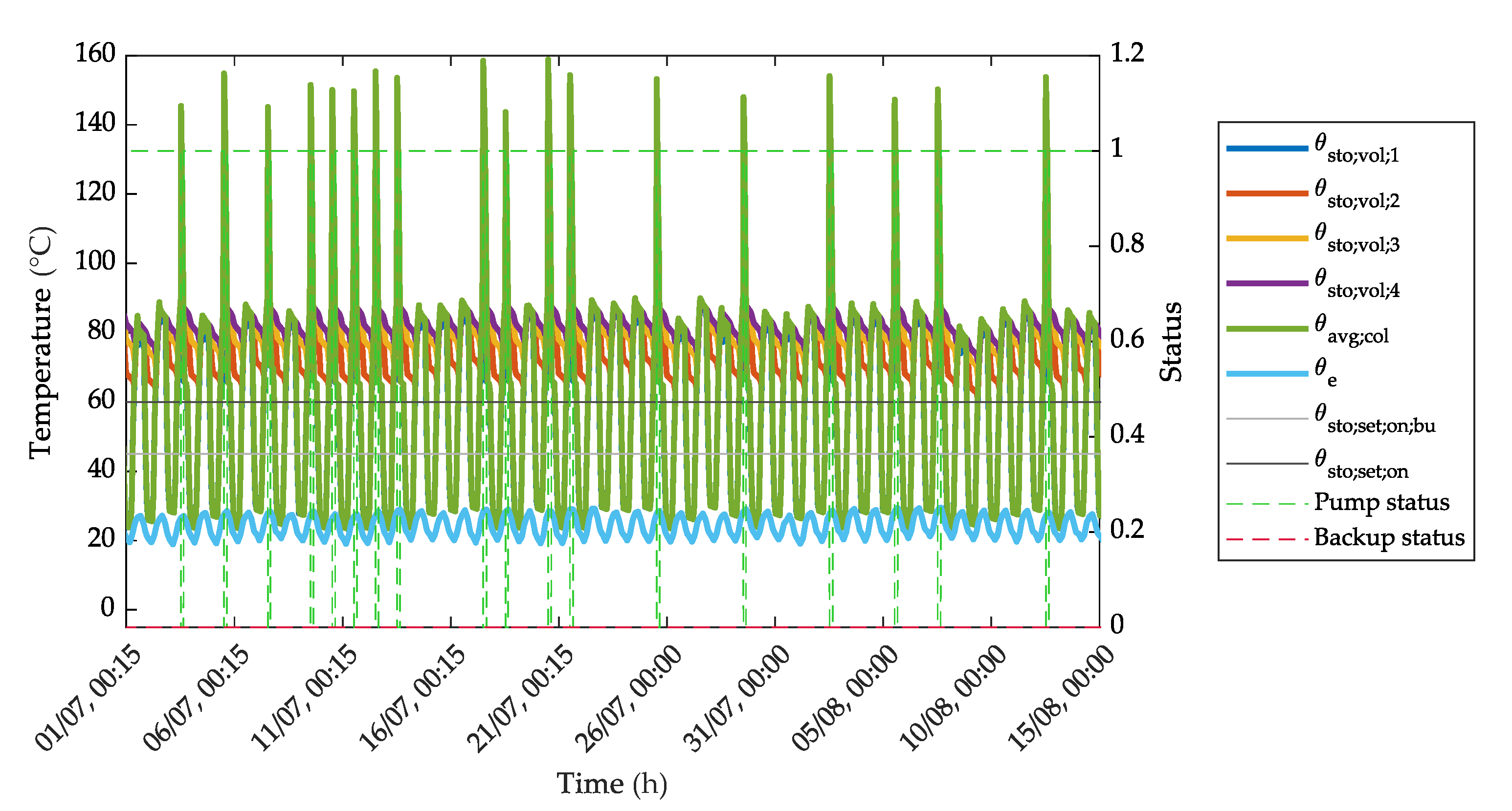
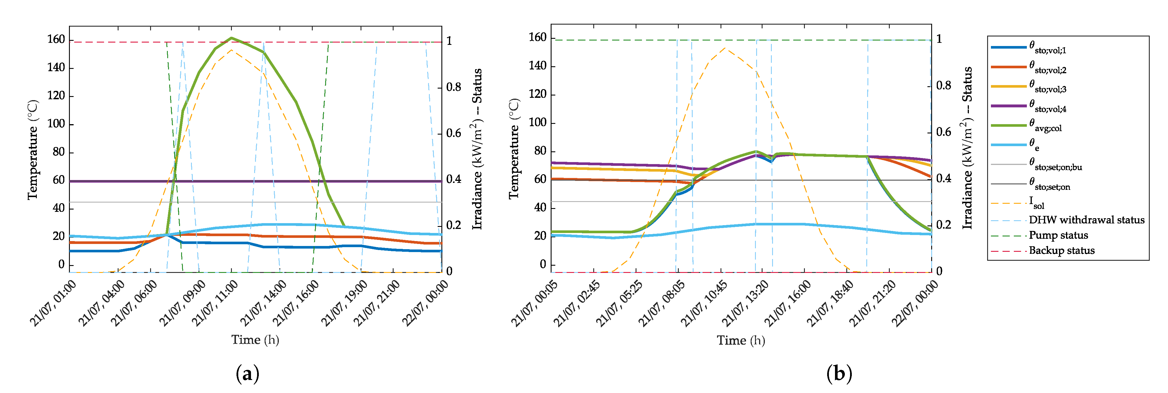
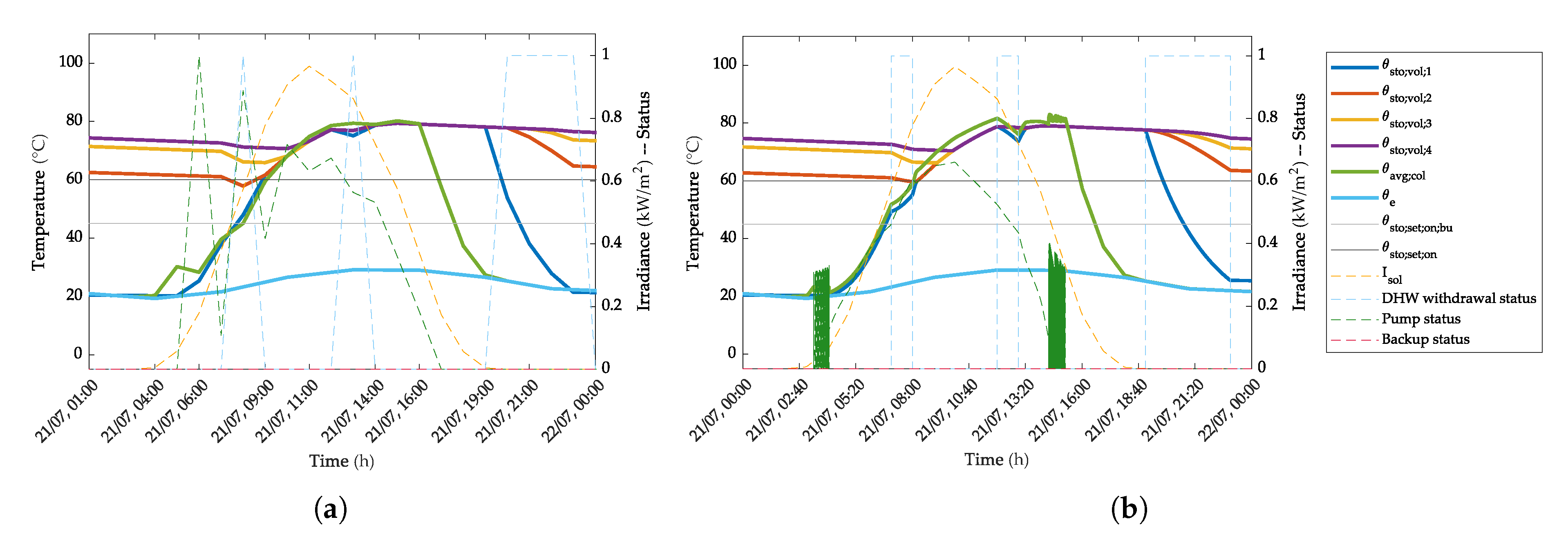
3.2. Modified Method: On-Off Control

Introducing pump-off when solar collector outlet temperature exceeds θ off = 90 C (case 2 in Table 1) apparently brings no changes with respect to the standard calculations. This is because the solar field temperature never reaches the safety threshold in a well-designed system with uniform load. However, stressing the system so to explore the influence of different parameters will highlight new information. For example, a smaller water volume may be set to investigate the possibility of keeping an existing storage tank instead of replacing/adding a new component. This might be the case of a renovation or, sometimes, of an attempt to minimize the storage footprint and save valuable space. Figure 9 shows the impact of using a 200 L storage tank instead of a 500 L volume over the temperature time series in a hot summer day.
The morning withdrawal impacts more on the storage temperature profile because of the smaller volume. At the maximum insolation the temperature of the solar field rises above the safety threshold and the pump stops, causing the rapid increase of the fluid temperature almost to the boiling value which is estimated to be around 168 C at 6 bar. While the pump is off, any DHW withdrawal is not compensated by solar energy flow and the temperatures in the storage tank fall. The pump is switched on only in late afternoon, at sunset, when little energy can be transferred to the DHW tank. As a result, the next withdrawal causes the temperatures to fall again. In particular, the temperature of layer 3 decreases below θ sto ; set ; on ; bu and the back-up source starts to heat the upper layers. In this configuration, 18% less energy is delivered to the storage tank with 70 h less of solar pump operation. On the opposite, the back-up works over 300 h more than in the 500 L original situation.
A similar result is obtained increasing the number of collectors from 4 to 6. This might represent the attempt to cover 100% of the needs April to September instead of May to August. The delivered solar energy increases by 14% and the back-up source works 30% less time, but the collectors overheat several times during the summer months (Figure 10).
When the solar fluid flow rate is reduced, the temperature of the solar field is higher and it increases more evidently during maximum insolation, because less heat is removed from the collectors. On the other hand, during morning withdrawals the temperature at the bottom of the storage tank decreases more rapidly because less solar energy is transferred to the water (Figure 11a). With one-tenth flow rate reduction, 11% less energy is delivered to the water over the year with the pump always running. The back-up is operated over 1000 h more, mainly concentrated in mid-seasons (Figure 11b).
An example of boiling occurrence is obtained by reducing the collector loop pressure from 6 bar to 3 bar, which causes the reduction of the boiling temperature. Repeating the simulation with 6 collectors, it was found that the fluid reaches the evaporation condition for three times in July (Figure 12).
The suitability of the designed system to a different location or to different consumption profiles can simply be evaluated by changing the input time series. The necessary information are hourly irradiance on the collector plane, expressed in watts per square meter, the hourly outdoor air temperature in degrees Celsius, and the hourly consumption in kilowatthours. As concerns weather data, different choices are possible, such as considering actual data or artificial reference years, but also defining “extreme” reference years to analyze the behavior of the system in particularly hot or cold periods (resilience assessment, [41]). Meaningful daily consumption cycles can be derived from the Regulation n. 814/2013 [42], where typical load profiles for water heater testing are given. Residential applications are represented by profiles M to XXL depending on the number of people. Thus varying the load profile over the year can be a possible way to take into account different water need conditions. Completely removing the load for a given summer interval can be used to predict the solar system behavior during a period of vacation, and to find possible solutions to protect the collectors from overheating. For example, in Figure 13a it can be observed that, when the load is removed, overheating occurs immediately and the pump is stopped the first or the second day. Figure 13b shows that, when a “discharge profile” is created with three close water withdrawals in the sunniest moment of the day, overheating is prevented.

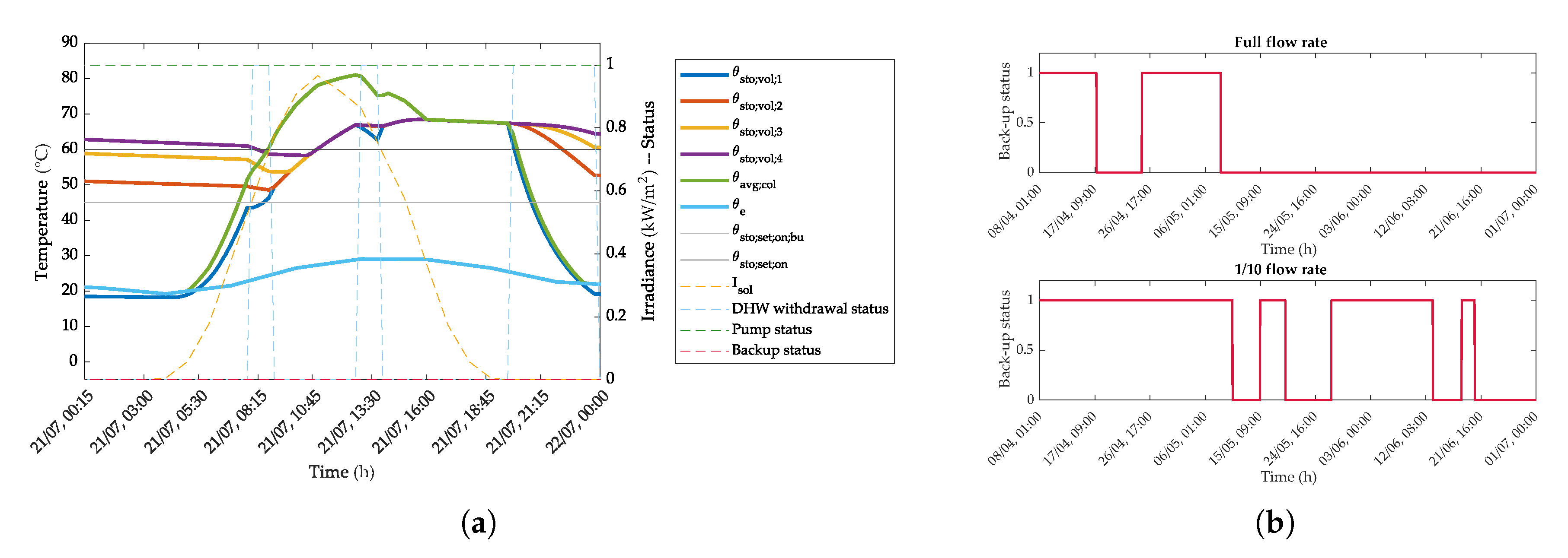
3.3. Influence of Control Strategy

Real-world controllers are more complex than just switching off the pump when a safety temperature is reached by the fluid. For example, a controller switches off the pump even when the temperature differential between solar field outlet and bottom layer of the storage tank (“reference differential”) is low. Moreover, with the widespread diffusion of electronic circulator pumps, even the simplest controller instantly modulates the speed of the pump based on the reference differential.
Such controls can be easily included in the code by calculating the flow rate based on the simulated temperatures, but a particular attention must be paid to the time step t ci . For example, if a lower threshold is introduced for the reference differential, below which the pump is switched off, the results of the simulation can be extremely different according to the time step, as shown in Figure 14.
The reason of this behavior lies in the quick variation of solar irradiance and in the too long time step compared to the circuit time constant: as the sun goes up, the temperature of the solar field grows rapidly; if the time step is too large the code may calculate a too large increase in the temperature of the collectors, and this would cause the pump to stop (Figure 14a). The result is completely misleading, as it would predict the waste of the solar energy and, paradoxically, the extensive intervention of the back-up generator in the sunniest days. A more realistic trend is shown in Figure 14b, where the only variation is the reduction of the time step from 1 h to 5 min.
A similar idea applies to the modulating control. A simple proportional model has been included in which the pump speed is varied linearly from 0% to 100% with the reference differential varying from 0 to 10 K. In this case, with hourly time step the oscillation of the proportional control results amplified when the sun rises and canceled when it sets (Figure 15a), whereas a more realistic behavior is represented in Figure 15b. The oscillations can be reduced by decreasing the slope of the proportionality curve, but in this case the pump would run at lower speeds and the delivered energy would decrease.
The pump is estimated to work only 38% of the year and almost always in modulation. Figure 16 shows the normalized distribution of the modulation levels over the pump yearly operation time. For example, the pump runs between 28% and 32% modulation for 9% of the running time, that is, for 3.4% of the year. With modulating control, the delivered solar energy decreases by less than 5%.

4. Discussion

The investigated method is a non-invasive addition to the standard framework, handled through an initial decision (“Calculation according to standard? Yes/No”) and the automatic check of the solution case. The benefit of this approach lies in that the impact of different parameters and design choices can be explored, and evaluations can be made on both hourly and annual analyses.
In (Figure 17) several simulations are compared in terms of solar pump and back-up annual operation times and solar energy delivered to the storage tank, whose values have been normalized over the corresponding values obtained from the standard simulation. The time step is one hour unless otherwise specified. For the “On-off” simulations, no lower reference differential threshold has been set. It can be observed that:
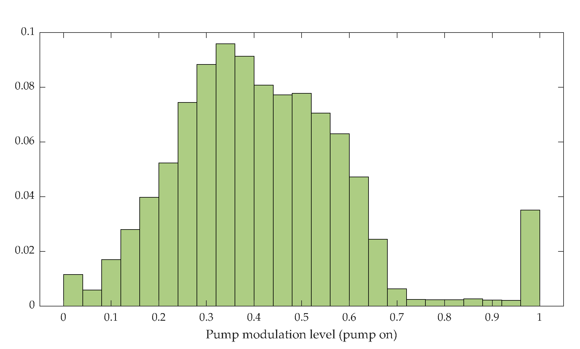
  • the pump works almost all the time except in the case of modulating control: moreover, with this control the pump works above 95% only 4% of the time; this highlights the benefit of efficient variable speed control for these applications using modern electronic pumps;
  • the reduction of the back-up operating time is linked to the increase in the captured solar energy, either due to the addition of collectors or to the sunnier geographical location (such as Lampedusa, one of the three Southern Italy’s localities in Italian climatic zone A): the higher the delivered solar energy, the lower the back-up operating time;
  • on the other hand, back-up operating time increases as the storage tank volume or the flow rate are decreased.
Figure 17 also shows the occurrences of pump stops, whose number increases as a result of inaccurate design choices like oversizing the solar field or undersizing the storage tank. Interestingly, the simulation in a sunnier location does not display significant overheating occurrences, the reason being that the selected location features higher temperatures and solar energy availability than Northern Italy in winter and mid-seasons (hence the strong reduction in back-up operating time), but comparable peak irradiances in summer.
It is worth remarking that the calculation code generates arrays containing values at each time step for all the relevant variables, including, among others: heat generated in the collector absorber; collector loop heat output (useful solar energy); collector efficiency; average collector temperature; average temperatures of the storage layers; pump status (0 or 1 in case of on–off control, or a value between 0 and 1 in case of modulating control); back-up energy input. These data, together with outdoor temperature, irradiance and energy demand for hot water, give the possibility to perform many detailed analyses and to look for correlations (for example, between weather data and stored energy, or between stratification and storage efficiency).

5. Conclusions

Thermal solar solution is an interesting way to exploit renewable sources, especially for domestic hot water preparation, but the system must be sized correctly to extend its lifespan as much as possible. EPB standards offer a sufficiently complete framework to perform dynamic calculations; adding the calculation for pump stops and modulation allows to evaluate the influence of several parameters and to use this approach also as a design tool. In particular, the simple addition of the simulation of pump stops due to overtemperature, the increased risk of stagnation deriving from increased solar field surface or decreased storage volume could be quantified. The solar fluid flow rate seems a less influencing parameter, although its reduction increases the operation time of the back-up heater in mid-seasons. The complete cancellation of domestic hot water needs to simulate periods of summer holidays shows that stagnation is very likely to occur in these circumstances unless precautions are taken, such as the installation of collector shutters or the timed discharge of part of the heated water. The enhanced method proposed in this work proved to be flexible and to provide helpful information. If detailed investigation on control strategy is to be performed, the time step must be reduced far below the hour in order to have realistic results.
Possible future developments include: modeling the superheating stage for those situations in which boiling cannot be avoided and for life cycle evaluations; applying the method to combined domestic hot water and space heating services; adding models of more complex control types, to estimate the associate pros and cons and electric power consumption; and, finally, modeling a more realistic back-up heater with a limited power, which might be very helpful in non-residential applications such as hotels, where the back-up heater is often a heat pump and where there are severe load peaks in the morning and in the evening.

Author Contributions

E.A.P. performed the literature survey and wrote the paper. B.G. implemented the scripts and carried out the simulations. L.S. conceived the study, supervised the work and reviewed the manuscript. All authors have read and agreed to the published version of the manuscript.

Funding

This research received no external funding.

Conflicts of Interest

The authors declare no conflict of interest.

Nomenclature

Symbols
t ci Calculation intervalh
QThermal energykWh
Q ˙ Thermal energy flowW
ISolar irradianceW/m 2
θ Temperature C
TAbsolute temperatureK
T * Reduced temperature of the collector(m 2 K)/W
A col Collector reference aream 2
η 0 Collector zero-loss efficiency-
η col Collector efficiency-
a 1 First-order heat loss coefficientW/(m 2 K)
a 2 Second-order heat loss coefficientW/(m 2 K 2 )
K hem Incidence angle modifier at 50 -
m c eff Effective heat capacity of the collectorJ/K
m ˙ Solar fluid mass flow ratekg/s
c p Solar fluid specific heatJ/(kg K)
VVolumeL
HHeat lossW/K
PElectric powerW
Subscripts
hHourly
mMonthly
avgAverage
boilBoiling
buBack-up
colCollector
disDistribution
eExternal
effEffective
evapEvaporated
lsLosses
minMinimum
ndNeed
offOff
onOn
outOutput
pmpPump
setThermostat setting
solSolar
stoStorage
volVolume
WDomestic water heating

References

  1. Ivancic, A.; Mugnier, D.; Stryi-Hipp, G.; Weiss, W. Solar Heating and Cooling Technology Roadmap; Technical Report; European Technology Platform on Renewable Heating and Cooling (RHC): Brussels, Belgium, 2014. [Google Scholar]
  2. Fabbri, K.; Tronchin, L.; Tarabusi, V. Energy retrofit and economic evaluation priorities applied at an Italian case study. Energy Procedia 2014, 45, 379–384. [Google Scholar] [CrossRef] [Green Version]
  3. Pezzutto, S.; Croce, S.; Zambotti, S.; Kranzl, L.; Novelli, A.; Zambelli, P. Assessment of the Space Heating and Domestic Hot Water Market in Europe—Open Data and Results. Energies 2019, 12, 1760. [Google Scholar] [CrossRef] [Green Version]
  4. Gautam, A.; Chamoli, S.; Kumar, A.; Singh, S. A review on technical improvements, economic feasibility and world scenario of solar water heating system. Renew. Sustain. Energy Rev. 2017, 68, 541–562. [Google Scholar] [CrossRef]
  5. Hernandez, P.; Kenny, P. Net energy analysis of domestic solar water heating installations in operation. Renew. Sustain. Energy Rev. 2012, 16, 170–177. [Google Scholar] [CrossRef]
  6. Harrison, S.; Cruickshank, C. A review of strategies for the control of high temperature stagnation in solar collectors and systems. Energy Procedia 2012, 30, 793–804. [Google Scholar] [CrossRef] [Green Version]
  7. Frank, E.; Mauthner, F.; Fischer, S. Overheating Prevention and Stagnation Handling in Solar Process Heating Applications; Technical Report A.1.2, International Energy Agency, Solar Heating and Cooling Programme (IEA SHC); International Energy Agency: Paris, France, 2012. [Google Scholar]
  8. Quiles, P.; Aguilar, F.; Aledo, S. Analysis of the overheating and stagnation problems of solar thermal installations. Energy Procedia 2013, 48, 172–180. [Google Scholar] [CrossRef] [Green Version]
  9. Botpaev, R.; Louvet, Y.; Perers, B.; Furbo, S.; Vajen, K. Drainback solar thermal systems: A review. Sol. Energy 2016, 128, 41–60. [Google Scholar] [CrossRef] [Green Version]
  10. Kessentini, H.; Castro, J.; Capdevila, R.; Oliva, A. Development of flat plate collector with plastic transparent insulation and low-cost overheating protection system. Appl. Energy 2014, 133, 206–223. [Google Scholar] [CrossRef]
  11. Eismann, R. Accurate analytical modeling of flat plate solar collectors: Extended correlation for convective heat loss across the air gap between absorber and cover plate. Sol. Energy 2015, 122, 1214–1224. [Google Scholar] [CrossRef] [Green Version]
  12. Hussain, S.; Harrison, S. Experimental and numerical investigations of passive air cooling of a residential flat-plate solar collector under stagnation conditions. Sol. Energy 2015, 122, 1023–1036. [Google Scholar] [CrossRef]
  13. Streicher, W. Minimising the risk of water hammer and other problems at the beginning of stagnation of solar thermal plants-A theoritical approach. Sol. Energy 2001, 69, 187–196. [Google Scholar] [CrossRef]
  14. Rossiter, W., Jr.; Godette, M.; Brown, P.; Galuk, K. An investigation of the degradation of aqueous ethylene glycol and propylene glycol solutions using ion chromatography. Sol. Energy Mater. 1985, 11, 455–467. [Google Scholar] [CrossRef]
  15. Clifton, J.; Rossiter, W., Jr.; Brown, P. Degraded aqueous glycol solutions: pH values and the effects of common ions on suppressing pH decreases. Sol. Energy Mater. 1985, 12, 77–86. [Google Scholar] [CrossRef]
  16. Monticelli, C.; Brunoro, G.; Trabanelli, F.; Frignani, A. Corrosion in solar heating systems. I. Copper behaviour in water/glycol solutions. Mater. Corros. 1986, 37, 479–484. [Google Scholar] [CrossRef]
  17. Monticelli, C.; Brunoro, G.; Trabanelli, G.; Frignani, A. Corrosion in solar heating systems. II. Corrosion behaviour of AA 6351 in water/glycol solutions. Mater. Corros. 1987, 38, 83–88. [Google Scholar] [CrossRef]
  18. Monticelli, C.; Brunoro, G.; Frignani, A.; Zucchi, F. Corrosion behaviour of the aluminium alloy AA 6351 in glycol/water solutions degraded at elevated temperature. Mater. Corros. 1988, 39, 379–384. [Google Scholar] [CrossRef]
  19. Dow Chemical Company. Engineering and Operating Guides for Ethylene and Propylene Glycol-based Heat Transfer Fluids; Technical Report; Dow Chemical Company: Midland, MI, USA, 2008. [Google Scholar]
  20. Hubbard-Hall. Cracked Glycols: An Underestimated Problem; Technical Report; Hubbard-Hall Inc.: Waterbury, CT, USA, 2010. [Google Scholar]
  21. Cholewa, T. Improving energy efficiency of hot water storage tank by use of obstacles. Rocz. Ochr. Sr. 2013, 15, 392–404. [Google Scholar]
  22. Fertahi, S.D.; Jamil, A.; Benbassou, A. Review on Solar Thermal Stratified Storage Tanks (STSST): Insight on stratification studies and efficiency indicators. Sol. Energy 2018, 176, 126–145. [Google Scholar] [CrossRef]
  23. Han, Y.; Wang, R.; Dai, Y. Thermal stratification within the water tank. Renew. Sustain. Energy Rev. 2009, 13, 1014–1026. [Google Scholar] [CrossRef]
  24. Chandra, Y.; Matuska, T. Stratification analysis of domestic hot water storage tanks: A comprehensive review. Energy Build. 2019, 187, 110–131. [Google Scholar] [CrossRef]
  25. Steinert, P.; Göppert, S.; Platzer, B. Transient calculation of charge and discharge cycles in thermally stratified energy storages. Sol. Energy 2013, 97, 505–516. [Google Scholar] [CrossRef]
  26. Kicsiny, R.; Farkas, I. Improved differential control for solar heating systems. Sol. Energy 2012, 86, 3489–3498. [Google Scholar] [CrossRef]
  27. Ntsaluba, S.; Zhu, B.; Xia, X. Optimal flow control of a forced circulation solar water heating system with energy storage units and connecting pipes. Renew. Energy 2016, 89, 108–124. [Google Scholar] [CrossRef] [Green Version]
  28. Valdiserri, P. Evaluation and control of thermal losses and solar fraction in a hot water solar system. Int. J. Low-Carbon Technol. 2018, 13, 260–265. [Google Scholar] [CrossRef]
  29. Klein, S.; Beckman, W.; Duffie, J. A Design Procedure for Solar Heating Systems. Sol. Energy 1976, 18, 113–127. [Google Scholar] [CrossRef]
  30. Klein, S.; Beckman, W.; Duffie, J. A Design Procedure for Solar Air Heating Systems. Sol. Energy 1977, 19, 509–512. [Google Scholar] [CrossRef] [Green Version]
  31. Shrivastava, R.; Kumar, V.; Untawale, S. Modeling and simulation of solar water heater: A TRNSYS perspective. Renew. Sustain. Energy Rev. 2017, 67, 126–143. [Google Scholar] [CrossRef]
  32. Duffie, J.A.; Beckman, W.A. Solar Engineering of Thermal Processes, 4th ed.; John Wiley & Sons Inc: Hoboken, NJ, USA, 2012. [Google Scholar]
  33. Camargo Nogueira, C.; Vidotto, M.; Toniazzo, F.; Debastiani, G. Software for designing solar water heating systems. Renew. Sustain. Energy Rev. 2016, 58, 361–375. [Google Scholar] [CrossRef]
  34. Gojak, M.; Ljubinac, F.; Banjac, M. Simulation of solar water heating system. FME Trans. 2019, 47, 1–6. [Google Scholar] [CrossRef]
  35. European Committee for Standardization (CEN). EN 15316-4-3–Energy Performance of Buildings-Method for Calculation of System Energy Requirements and System Efficiencies-Part 4-3: Heat GeneratIon SystemS, ThermaL Solar anD Photovoltaic Systems, Module M3-8-3, M8-8-3, M11-8-3; European Committee for Standardization: Bruxelles, Belgium, 2017. [Google Scholar]
  36. Socal, L. The new dynamic hourly method for the calculation of the envelope needs (Il nuovo metodo orario dinamico per il calcolo dei fabbisogni dell’involucro). Progetto 2000 2018, 54, 24. (In Italian) [Google Scholar]
  37. REHVA. EPB Standards-Energy Performance of Buildings Standards. Available online: https://www.rehva.eu/activities/epb-center-on-standardization/epb-standards-energy-performance-of-buildings-standards (accessed on 9 August 2019).
  38. European Committee for Standardization (CEN). EN 15316-5—Energy Performance of Buildings—Method for Calculation of System Energy Requirements and System Efficiencies—Part 5: Space Heating and DHW sTorage Systems (Not Cooling), Module M3-7, M8-7; European Committee for Standardization: Bruxelles, Belgium, 2017. [Google Scholar]
  39. Photovoltaic Geographical Information System (PVGIS). Available online: https://ec.europa.eu/jrc/en/pvgis (accessed on 26 November 2019).
  40. Siuta-Olcha, A.; Cholewa, T. Research of thermal stratification processes in water accumulation tank in exploitive conditions of solar hot water installation. In Proceedings of the 41st International Congress and Exhibition on Heating, Refrigerating and Air Conditioning, Belgrade, Serbia, 1–3 December 2010. [Google Scholar]
  41. Pernigotto, G.; Prada, A.; Gasparella, A. Extreme reference years for building energy performance simulation. J. Build. Perform. Simul. 2019. [Google Scholar] [CrossRef]
  42. European Commission. Commission Regulation (EU) No 814/2013 of 2 August 2013 implementing Directive 2009/125/EC of the European Parliament and of the Council with Regard to EcodesigN Requirements for Water Heaters and Hot Water Storage Tanks Text with EEA Relevance; European Commission: Brussels, Belgium, 2013. [Google Scholar]
Figure 1. Energy flows in a forced-circulation solar system.
Energies 13 00266 g001
Figure 2. Diagram for the use of f-chart method to determine monthly solar fraction for sizing purpose.
Energies 13 00266 g002
Figure 3. Diagram for hourly calculation according to EN 15316-4-3 and EN 15316-5.
Energies 13 00266 g003
Figure 4. Diagram for hourly calculation of the stratified storage tank according to EN 15316-5.
Energies 13 00266 g004
Figure 5. Monthly balance from f-chart-based method simulation. Useful solar energy: min ( Q sol ; loop ; out ; Q sto ; out ) . Remaining DHW need: max ( Q sto ; out Q sol ; loop ; out ; 0 ) . Excess solar energy: max ( Q sol ; loop ; out Q sto ; out ; 0 ) .
Energies 13 00266 g005
Figure 6. Results from standard simulation over a year. Time step 1 h. Solar pump running when Q sol ; loop ; out 3 · P sol ; pmp · 10 3 · t ci . Storage layers numbered from bottom (1) to top (4).
Energies 13 00266 g006
Figure 7. Results from standard simulation: (a) a winter day; (b) a summer day; (c) spring mid-season; (d) fall mid-season. Solar pump running when Q sol ; loop ; out 3 · P sol ; pmp · 10 3 · t ci .
Energies 13 00266 g007
Figure 8. Annual distribution of energies (simulation according to standard).
Energies 13 00266 g008
Figure 9. The effect of a smaller storage tank on system temperatures in a hot summer day. Time step: 15 min.
Energies 13 00266 g009
Figure 10. The effect of larger solar surface on system temperatures in summer months. Time step: 15 min.
Energies 13 00266 g010
Figure 11. The effect of lower flow rate (a) on system temperatures in a hot summer day, and (b) over the back-up switch-off in spring mid-season. Time step: 15 min.
Energies 13 00266 g011
Figure 12. The effect of lower load pressure on system temperatures with an oversized solar field in summer, resulting in fluid boiling. Time step: 15 min.
Energies 13 00266 g012
Figure 13. (a) Overheating at the beginning of a summer vacation period (no load). (b) Simulation with custom discharge profile. Time step: 1 h.
Energies 13 00266 g013
Figure 14. The effect of the time step on simulations featuring lower reference differential threshold (0 K): (a) t ci = 1 h, and (b) t ci = 5 min.
Energies 13 00266 g014
Figure 15. The effect of the time step on simulations featuring modulating control: (a) t o c i = 1 h, and (b) t o c i = 5 s.
Energies 13 00266 g015
Figure 16. Normalized distribution of modulation levels when the pump is on (38% of time over the year). Bin width: 4%.
Energies 13 00266 g016
Figure 17. Comparison between yearly simulation results in different conditions. Pump working hours, back-up working hours and delivered solar energy are normalized over the corresponding values obtained for “Standard” simulation.
Energies 13 00266 g017
Table 1. Calculation types according to collector temperature value.
Conditions at Time Step h 1
CasePump State θ col ; avg < θ off θ col ; avg < θ boil Calculation Type
1OnYesYesSteady (to standard)
2OffNoYesExponential
3OffNoNoBoiling
Table 2. Main component characteristics.
CharacteristicSymbolValueUnit
Collector areaA1.9m 2
Peak collector efficiency η 0 0.8-
First order collector heat loss coefficient a 1 4.35W/(m 2 K)
Second order collector heat loss coefficient a 2 0.01W/(m 2 K 2 )
Incidence angle modifier K hem 0.91-
Collector volume content V col 1.5L
Storage volume V sto 500L
Storage heat loss H sto ; ls 2.44W/K

