Article

Direct Torque Control of PMSM with Modified Finite Set Model Predictive Control

1
College of Electrical Engineering and Information Engineering, Lanzhou University of Technology, Lanzhou 730050, China
2
Key Laboratory of Gansu Advanced Control for Industrial Processes, Lanzhou University of Technology, Lanzhou 730050, China
3
National Demonstration Center for Experimental Electrical and Control Engineering Education, Lanzhou University of Technology, Lanzhou 730050, China
4
Gansu Natural Energy Research Institute, Lanzhou 730046, China
*
Author to whom correspondence should be addressed.
Energies 2020, 13(1), 234; https://doi.org/10.3390/en13010234
Submission received: 7 November 2019 / Revised: 20 December 2019 / Accepted: 24 December 2019 / Published: 3 January 2020
(This article belongs to the Special Issue Advances in Rotating Electric Machines)

Abstract

:
A direct torque control (DTC) with a modified finite set model predictive strategy is proposed in this paper. The eight voltage space vectors of two-level inverters are taken as the finite control set and applied to the model predictive direct torque control of a permanent magnet synchronous motor (PMSM). The duty cycle of each voltage vector in the finite set can be estimated by a cost function, which is designed based on factors including the torque error, maximum torque per ampere (MTPA), and stator current constraints. Lyapunov control theory is introduced in the determination of the weight coefficients of the cost function to guarantee stability, and thus the optimal voltage vector reference value of the inverter is obtained. Compared with the conventional finite control set model predictive control (FCS-MPC) method, the torque ripple is reduced and the robustness of the system is clearly improved. Finally, the simulation and experimental results verify the effectiveness of the proposed control scheme.

1. Introduction

Permanent magnet synchronous motor (PMSM) direct torque control (DTC) has been widely used in industry due to its simple control structure, fast dynamic response, and high efficiency [1]. However, the traditional DTC control results in large torque ripple due to the insufficient switching frequency of the inverters and two nonlinear hysteresis comparators [2,3].
To solve the problem of torque ripple, many scholars have put forward many improved methods. An improved method is calculating the effective voltage vector action time in real time to ensure the minimum torque ripple by the current torque error [4,5,6]. This method reduces the torque ripple to a certain extent, but the calculation process is complicated. At present, voltage space vector modulation (SVM) is also introduced into DTC [7,8]. This method can effectively reduce the torque ripple, but it cannot eliminate the steady-state error of the torque. At the same time, the calculation process is highly dependent on the parameters of the motor and has poor robustness.
As a real-time online optimization control method, model predictive control (MPC) has received extensive attention in the field of electric drives and power converters due to its high dynamics and resistance to parameter disturbance [9,10]. The method of finite control set MPC (FCS-MPC) directly utilizes the discreteness of inverter output voltage and the finiteness of switching state; at the same time, it does not need modulation and has a small amount of computation, which makes it a hot research topic in the field of power electronics [11,12]. In [13], on the premise that the flux linkage and torque of the motor are limited within the target range, a longer prediction step is selected to optimize the switching frequency of the inverter. A strategy of separate control of transient and steady state are adopted to reduce the switching frequency of inverter [14]. Mayne [15] proposed an FCS-MPC algorithm with model error compensation which enhances the robustness of the system. In [16], FCS-MPC method is applied in a grid-connected converter, and the stability of the control system is proved by Lyapunov stability theory. In addition, the virtual voltage vector is also integrated into FCS-MPC architecture, and the optimal voltage vector is preselected by using the results of Lyapunov stability theory. This method reduces the number of possible voltage vectors from 38 to 10, thus reducing the computational burden of the controller.
The cost function of FCS-MPC is the key to realizing the optimal selection of the voltage vector, which can be established according to the control targets, the system model based predictive variables, and the reference variables [17]. Depending on the control situation, it is also necessary to include system constraints. The cost function can contain multiple control objectives, variables, and constraints. Correct design of reasonable weight coefficients is very important for selecting the voltage vectors and governing the switching sequence of the inverter based on predictive current control of the PMSM with the FCS model [18,19].
The main contribution of this paper is to combine Lyapunov function theory with FCS-MPC to reduce torque ripple. Among them, the operating conditions of MTPA and torque tracking are guaranteed by using cost function. The Lyapunov function theory is introduced in the calculation of the finite set voltage vector duty cycle to obtain the optimal voltage vector. The simulation and experimental results show that the method achieves fast torque response and torque ripple minimization.

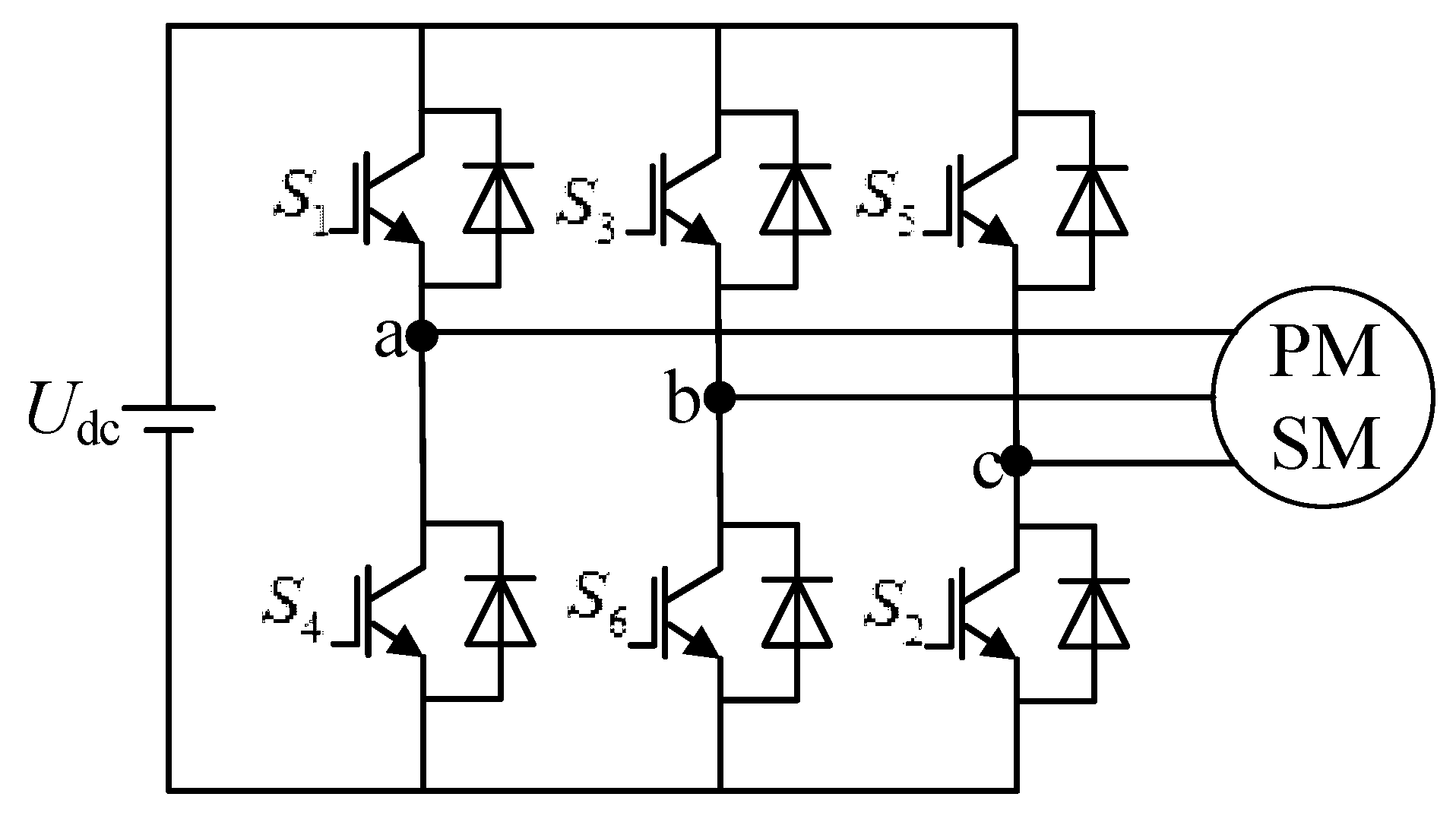
2. Discrete Mathematical Model of PMSM and Drive

The main circuit of the electric drive system under consideration is illustrated in Figure 1, which also corresponds to the experimental system layout. The PMSM has the characteristics of being multivariable and nonlinear and has strong coupling [20]. In order to simplify the mathematical model of PMSM, the following assumptions are made: (1) Y-shaped connection of stator windings, symmetrical distribution of three-phase windings, and space difference of each winding is 120°. (2) Eddy current loss, hysteresis loss, and the change of motor parameters are neglected. (3) It is assumed that permanent magnets on the rotor generate a main magnetic field in the stator–rotor airgap (the magnetic field is distributed sinusoidally along the circumference of the airgap) 22. So the continuous time model for PMSM in the d–q coordinate system can be described as:
L d d i d d t = ( u d R i d + ω L q i q ) ,
L q d i q d t = ( u q R i q ω L d i d ω ψ f ) ,
T e = 1.5 p ( ψ f + ( L d L q ) i d ) i q ,
where u d , u q , i d and i q are the stator voltages and currents, R is the stator winding resistance, L d and L q are the d- and q-axes inductances, ψ f is the flux linkage of the rotor, p is the number of pairs of poles, ω is the mechanical angular speed, and T e is the electromagnetic torque. i q is proportional to the electromagnetic torque and i d is proportional to the reactive power. A predictive current control scheme is thus formed in which the reference current is generated by an external speed control loop.
Discretize the mathematical model of PMSM to obtain the necessary conditions for model prediction. Since the sampling time T s is sufficiently small, the Euler approximation is used for the stator current derivative di/dt of the sampling time T s .
d i d t = i ( k + 1 ) i ( k ) T s ,
where T s is the sampling period. Then, the discrete current model of the PMSM is obtained:
L d i d k + 1 = ( L d T s R ) i d k + T s ω L q i q k + T s u d k ,
L q i q k + 1 = ( L q T s R ) i q k T s ω L d i d k T s ω ψ f + T s u q k ,
T e k + 1 = 1.5 p i q k + 1 [ ψ f + ( L d L q ) i d k + 1 ] .
The commutation process of two-level voltage source inverters is accomplished by use of DC bus. The switching state can be represented by the switching signals S a and S b and switching on and off on different bridge arms. The upper and lower switches of each bridge arm of the inverter cannot be turned on at the same time to prevent short circuit S c , as shown in Table 1:
From the above table, the vector form function of the switching state of the three-phase bridge arm ( S ) is as follows:
S = 2 3 ( S a + a S b + a 2 S c ) ,
where a = e j 2 π / 3 . The relationship between output voltage vector with the switch state can be defined as:
U o u t = S U d c = 2 3 U d c ( S a + a S b + a 2 S c ) ,
where U d c is the DC source voltage and U o u t is the output voltage of the inverter.
Considering the different switching states of the inverters, eight different voltage vectors are obtained, as shown in Table 2. It is noted that V 0 = V 7 , resulting in a finite set of seven different voltage vectors in the plane.

3. Predictive Control Based on Duty Cycle

Within one sampling interval, the cost function values that correspond to the seven voltage vectors are calculated by the FCS. The switching state that minimizes the cost function is chosen as the switching state of the inverter. The process of model prediction optimization is shown in Figure 2, where x , x p , and x * are the torque of the real response, the predicted value, and the reference value, respectively. If the corresponding x(k) is the best value at time k, the cost function value x(k + 1) corresponding to the seven voltage vectors is calculated at time (k + 1), and the seven calculated cost functions values are compared with reference values, where the closest is to be the optimal solution at the moment (k + 1). V4 is the control signal of the voltage vector corresponding to the optimal value of the time (k + 1). In the same way, V3 should be selected as the optimal control signal at time (k + 2) [12].

3.1. Design of Cost Function

The maximum torque/current control (MTPA) consumes the minimum stator current at the same electromagnetic torque output, which is usually used in interior PMSM systems. The space vector analysis of PMSM in the d–q coordinate system is shown in Figure 3. Assuming that the stator current vector i s leads q axis β , the current component in the d–q coordinate system is as follows:
{ i d = | i s | sin β i q = | i s | cos β i s = i d 2 + i q 2 ,
T e = 1.5 p [ ψ f i s cos β ( L d L q ) i s 2 cos β sin β ] .
If the amplitude of the stator current of the PMSM is a constant value, it can be concluded that the electromagnetic torque of the motor is only related to β . In order to find the maximum value of the torque, that is, to satisfy the MTPA condition, and calculate Equation (11) with β as a variable, the following relationship is obtained:
d T e d β = ψ f i s sin β ( L d L q ) i s [ cos β 2 sin β 2 ] = 0 .
Because i s and β satisfy the Pythagorean theorem, the relationship of i d and i q under the MTPA condition can thus be derived as follows:
i d + L d L q ψ f ( i d 2 i q 2 ) = 0 .
The most important part of MPC is the cost function design. The cost function is expressed in orthogonal coordinates and considering the torque tracking, MTPA condition, and current constraint:
J ( k ) = K T J T ( k ) + K M J M ( k ) + K C ( J C 1 ( k ) + J C 2 ( k ) ) ,
where K T , K M , and K C are the weighting factors of the cost function and are positive real numbers. The main aim of the MPC is to minimize the torque error. Thus, the cost for the error J T ( k ) is:
J T ( k ) = ( T e * T e k + 1 ) 2 .
Since high currents lead to large losses, J M ( k ) is to have a low absolute current:
J M ( k ) = ( i d k + L d L q ψ F ( ( i d k ) 2 ( i q k ) 2 ) ) 2 .
Tertiary control goals can be added in order to ensure the operational safety of the system. J C 1 ( k ) denotes the current limit, and the current amplitude of the system must be smaller than the maximum allowable value I max .
J C 1 ( k ) = { 0 ( I max ( i d k ) 2 + ( i q k ) 2 ) ( I max ( i d k ) 2 + ( i q k ) 2 ) 2 ( I max < ( i d k ) 2 + ( i q k ) 2 )
To make the point of the cost function converge to the parabola on the left side of the i q axis, as shown in Figure 3. Adding current constraints J C 2 ( k ) to the cost function:
J C 2 ( k ) = { 0 , ( i d k 0 ) ( i d k ) 2 , ( i d k > 0 ) .
To ensure current constraints and avoid control variables converging to the wrong MTPA curve, K C K T , K M should be satisfied. For the choice of K T and K M , K T + K M = 1 can be made. A larger value of K T leads to faster convergence of the torque, while a larger value of K M indicates that the MTPA state converges quickly. K T > K M can be selected [21] to achieve a fast torque response.

3.2. Duty Cycle Calculation

The duty cycle of each voltage vector in a finite set is calculated by Lyapunov function to eliminate torque and current ripple. Without considering the current limitation, that is, ignoring J C 1 ( k ) and J C 2 ( k ) , the Lyapunov function is expressed as follows:
V ( k + 1 ) = k T J T ( k + 1 ) + k M J M ( k + 1 ) .
In order to optimize the operation of the PMSM, the condition V ( k + 1 ) = 0 must be fulfilled to ensure T e k + 1 = T e * and its current operating point is on the MTPA curve. In addition, the condition d V ( k + 1 ) / d t = 0 indicates that the PMSM is operating at the optimum state.
Lemma 1.
Defining the function of the current:
f ( i d , i q ) = i d + ( L d L q ) ( i d 2 q 2 ) / ψ f
If the torque of the PMSM is kept at a nonzero constant value, the function f ( i d , i q ) is a strict monotonic function along the constant torque curve. The correlative poof is introduced in the Appendix A.
With the help of the function f ( i d , i q ) , the stator current trajectory is shown in Figure 4. Point A is the initial point; the trajectory first reaches the point B along the constant torque curve and then reaches the point C along the MTPA curve with the condition V ( k ) = 0 . When the current trajectory is along A B to B C , the Lyapunov function is strictly decreasing.
Lemma 2.
Under the initial condition of the PMSM, if the back EMF of the PMSM is within the voltage limit range of the inverter, there exists a feasible voltage vector u d q * that fulfills:
d V ( k + 1 ) / d t 0 .
Lemma 3.
For a given current dynamics:
d i d q k + 1 d t = A i d q k + 1 + B u d q k + 1 + E ,
where A = [ R L d     ω L q L d ω L d L q   R L q ] , B = [ 1 L d   0 0     1 L q ] , E = [ 0 ω ψ f L q ] .
If the back EMF of the PMSM is within the voltage limit range of the inverter, then at least one voltage vector is satisfied:
d V ( k + 1 ) d t = V ( k + 1 ) i d q k + 1 ( A i d q k + 1 + B u d q k + 1 + E ) 0 .
The proofs of Lemma 2 and Lemma 3 are introduced in the Appendix A.
In order to minimize the ripple of the PMSM current and torque, the Lyapunov function is expected to keep V = 0 and d V ( k + 1 ) / d t = 0 in a steady state. The duty cycle of each voltage vector satisfying the desired requirement is calculated as follows:
T d u t y , k + 1 j = { T σ   ,         d V ( K + 1 ) d t > 0           0   ,             d V ( K + 1 ) d t = 0   V ( K + 1 ) d V ( k + 1 ) / d t     ,   d V ( K + 1 ) d t < 0 ,
Here, T σ T s is a time constant. The voltage vector with d V ( k + 1 ) / d t > 0 has to be taken into account in the FCS-MPC, and then the current reaches the limit, T σ is introduced, and the current constraint plays a major role in the cost function. When there is disturbance in the PMSM system, such as machine parameter drift and voltage error in the inverter, we also need to select a smaller T σ to compromise the disturbance at this point. When the PMSM model and the prediction are accurate, T σ = 0 is the ideal value for the ripple reduction. All voltage vectors u d q , k + 1 j with d V ( k + 1 ) / d t < 0 are candidates to minimize the cost function.

3.3. Finite Control Set Model Prediction

Finally, the optimum output voltage which can be realized by the SVPWM is obtained by Equation (23). Only when voltage u d q , k + 1 j acts on the PMSM will it affect the torque, that is, to ensure the implementation of MTPA and d V ( k + 1 ) / d t = 0 . It is noteworthy that setting the optimal duty cycle T d u t y k + 1 equal to T s in the transient state of the proposed control strategy can minimize the cost function. Therefore, under the same sampling frequency, the torque response of the new strategy is as fast as that of the traditional FCS-MPC. In steady state, d V ( k + 1 ) / d t = 0 can be maintained. Therefore, current ripple and torque ripple can be minimized. Figure 5 is a block diagram of the predictive direct torque control algorithm of the FCS-MPC proposed in this paper.
[ u d k + 1 u q k + 1 ] = ( 1 T d u t y k + 1 ) | R i d k + 1 ω L q i q k + 1 R i q k + 1 ω L d i d k + 1 + ω ψ F | + T d u t y k + 1 | u d j , k + 1 u q j , k + 1 |

4. Simulation Results

In order to investigate the effectiveness and feasibility of the proposed method, the FCS-MPC of the surface-mounted PMSM based on MATLAB/Simulink software was built. Then, it was compared with that of the classical FCS-MPC method. The parameter settings are shown in Table 3.

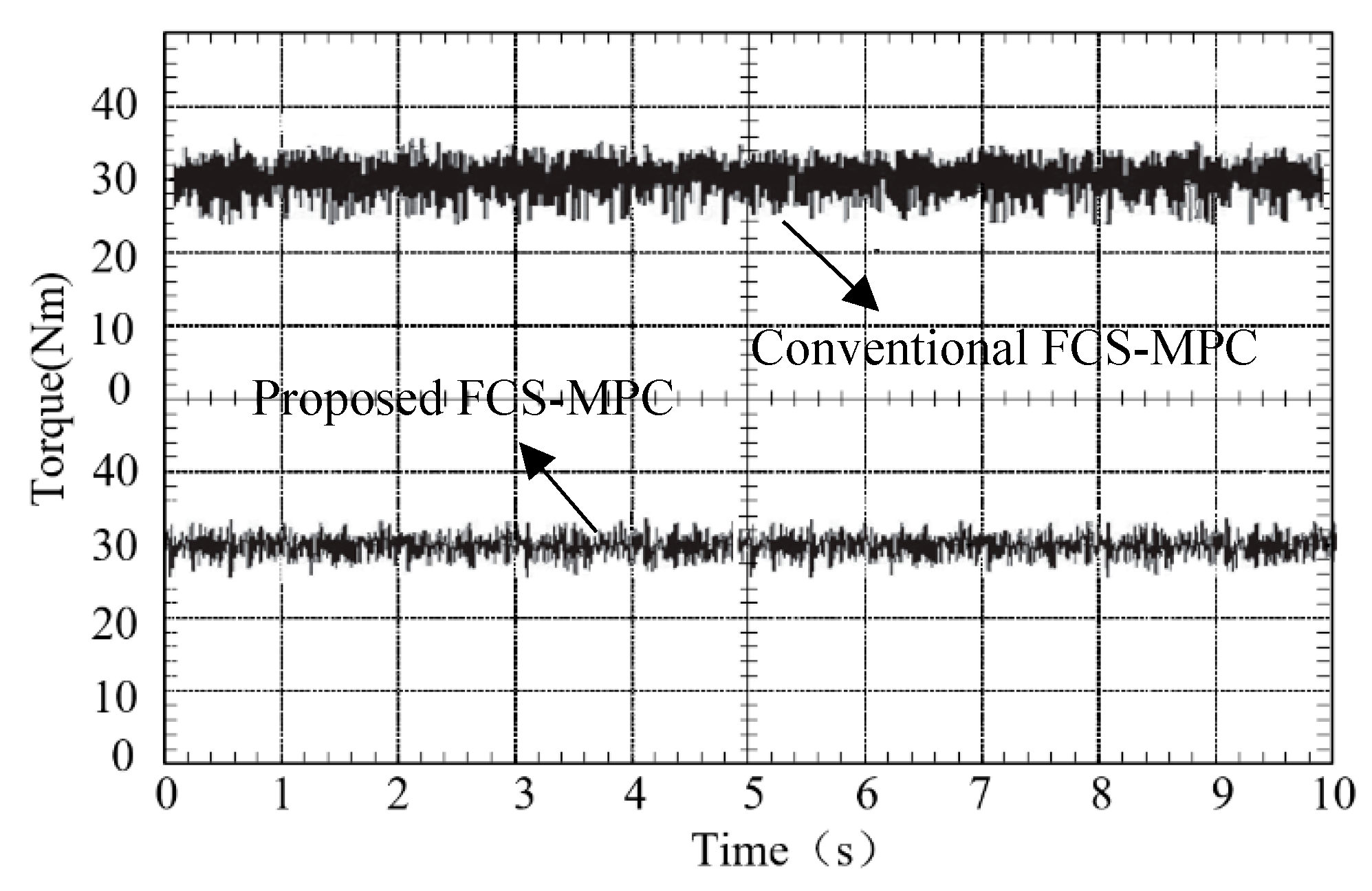
4.1. Steady-State Operation

Figure 6 shows the simulation results of traditional FCS-MPC and improved FCS-MPC under steady-state conditions. The reference value of motor speed is set to 500 rpm, and the load torque is 20 N⋅m. As can be seen from the figure, compared with conventional FCS-MPC, the torque ripple of the improved method is significantly reduced. In Figure 6, the average values of the torque ripples of proposed (0.9 N⋅m) are smaller compared to those of conventional FCS-MPC (3 N⋅m) under the same conditions. It is noted that, in this paper, torque ripples are calculated by the following equation [22]:
T r i p = 1 N i = 1 N ( T e T a v e ) 2 ,
where N is the number of samples and T a v e is the average value of the torque.

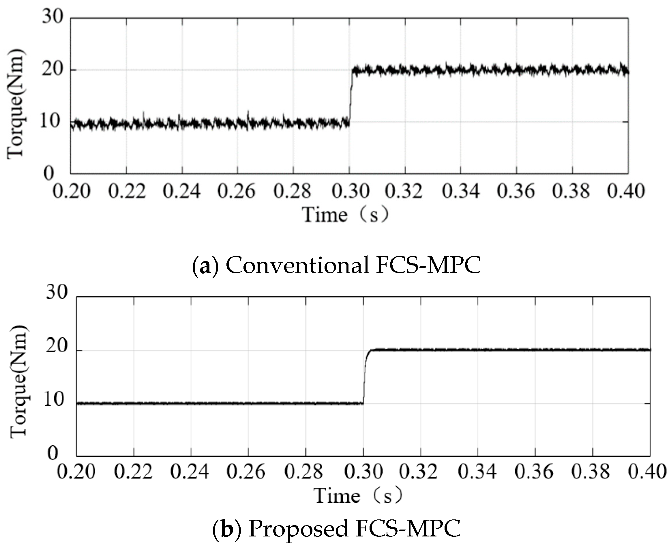
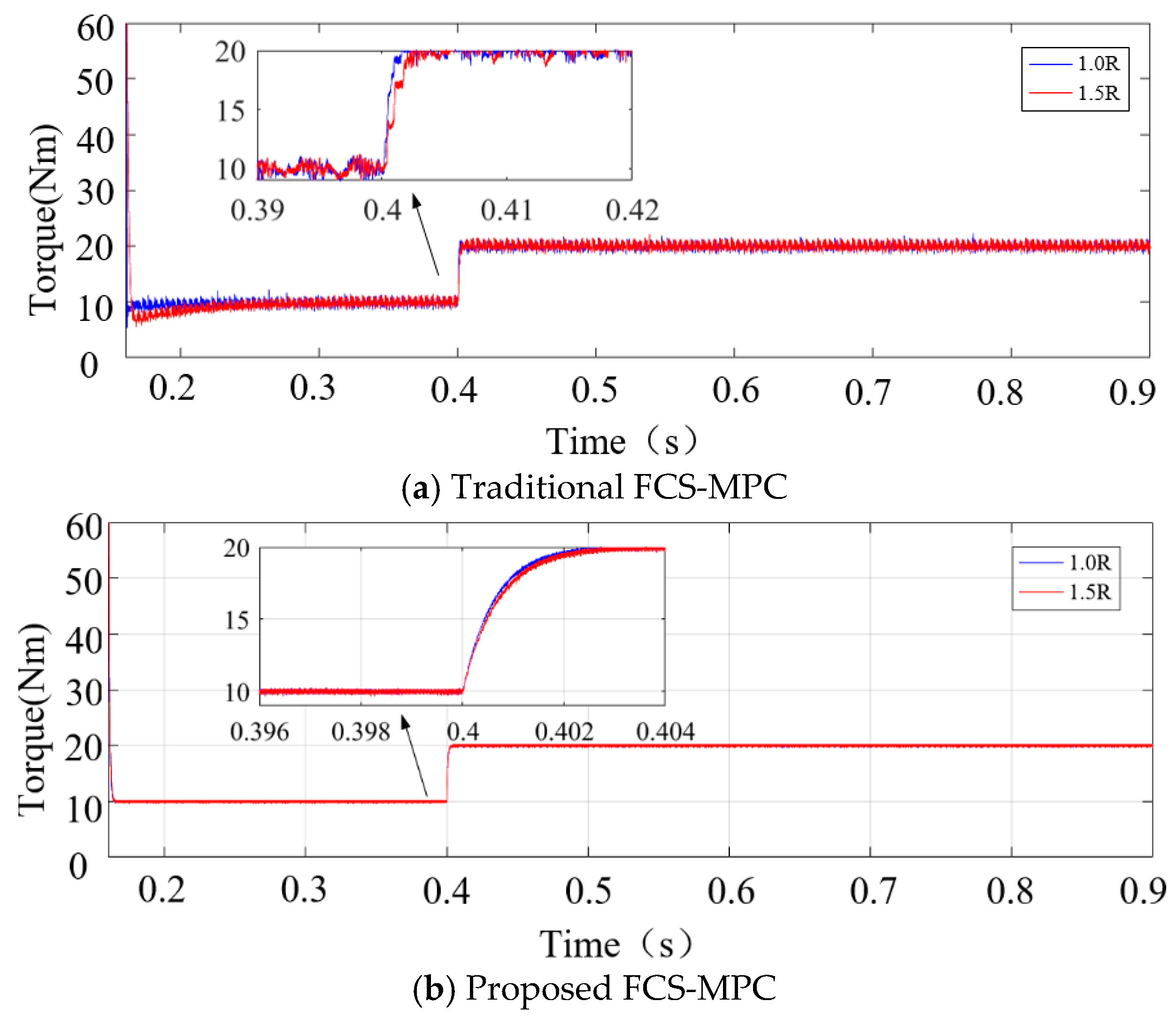
4.2. Dynamic Response

In order to compare the torque dynamic, a magnified view of the torque response is shown in Figure 7. From Figure 7, we can see that the torque suddenly increases from 10 to 20 N⋅m in only 0.003 s, and in the process of torque mutation, the conventional FCS-MPC method has obvious overshoot. Compared with the conventional FCS-MPC, the improved method has faster dynamic response because the motor adopts optimized duty cycle modulation in the whole control cycle.

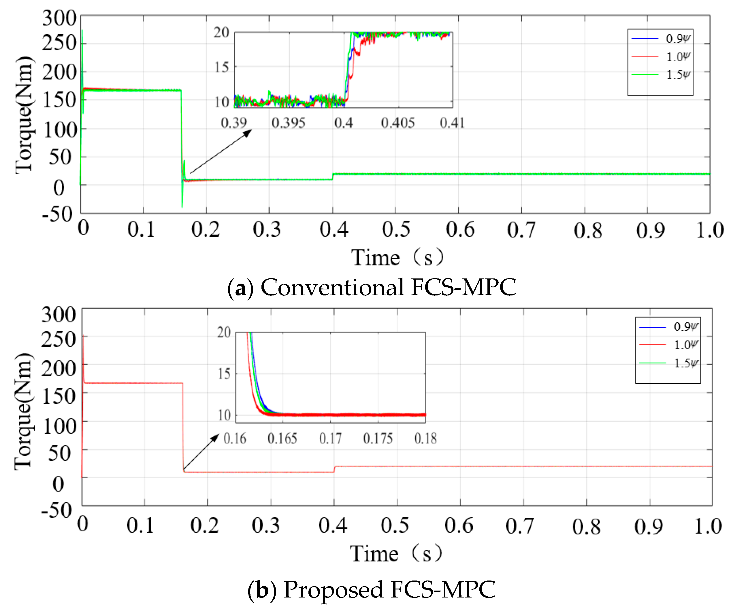
4.3. Motor Parameter Robustness

As we all know, a temperature rise of the motor will cause the stator internal resistance to increase. The influence of internal resistance on the torque is discussed in this paper. The torque waveforms of the two control methods in the condition of rated stator resistance (the blue solid line) and 1.5-times the rated value (the red dashed line) are given in Figure 8a,b, respectively. It is noticeable that slight torque ripples occur under the conventional FCS-MPC method when the resistance increases, while the proposed FCS-MPC control has better robustness in which the torque is insensitive to the resistance change. However, when entering a steady state, the two control systems are not affected by internal resistance changes.
Almost all permanent magnet devices, including permanent magnet motors, will exhibit the demagnetization phenomenon in varying degrees due to factors such as the working environment and usage time. The effect of changes in the motor flux on torque is also discussed. Figure 9a,b shows the torque waveforms of the two control methods when the rotor flux is 0.9-times the rated value, equal to the rated value, and 1.1-times the rated value, to simulate permanent magnet motors that have been used for a long time, used normally, and newly manufactured. As shown in Figure 9, the blue point line is 0.9-times the rated flux, the red solid line is the rated flux, and the green dotted line is 1.5-times the rated flux. Evidently, the conventional FCS-MPC for the change of flux is the change of the maximum torque. However, the improved predictive control is insensitive to the flux change.
For a mechanical load, the oscillation of torque is very bad for the shaft and load of the motor. Therefore, it can be seen from the simulation waveforms of the above two sections that the robustness of predictive control to parameter changes is better than that of conventional FCS-MPC. In theory, the switch meter of direct torque control is fixed in advance and cannot be adjusted according to the running state of the motor. Therefore, the robustness of direct predictive control to parameter changes is better than that of direct torque control, which is also consistent with the previous prediction results.

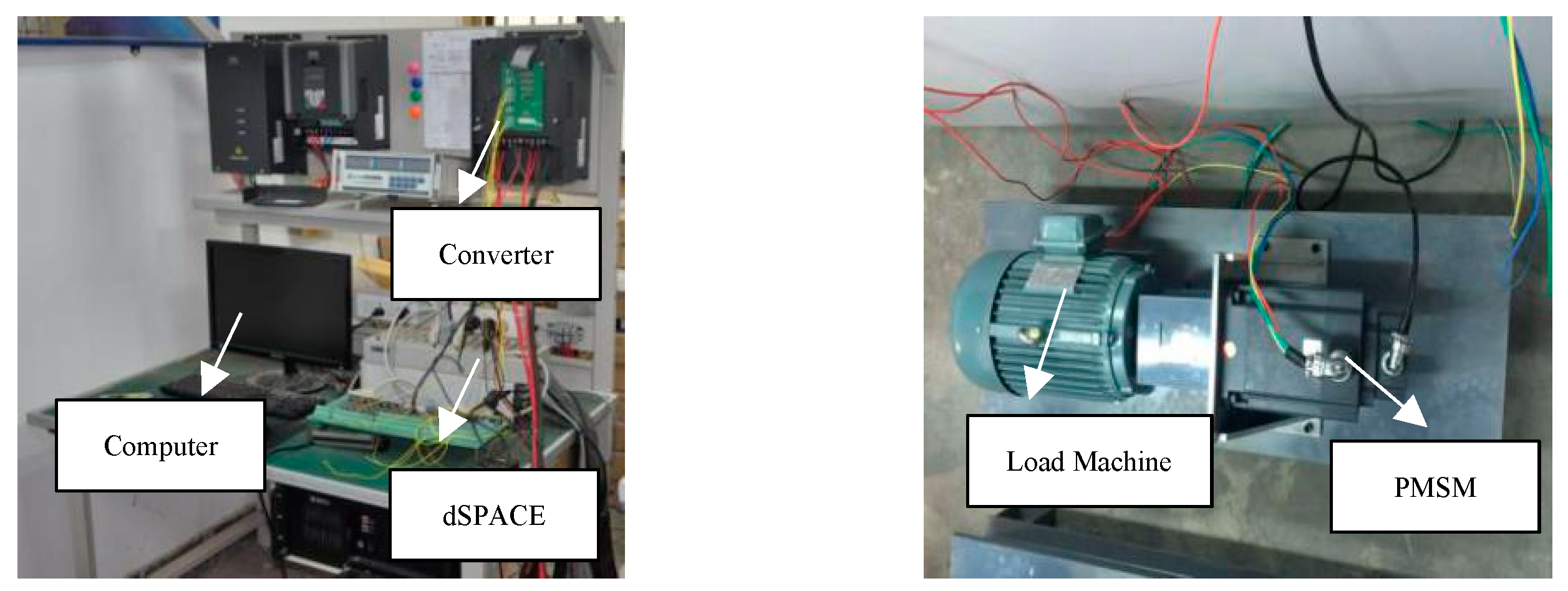
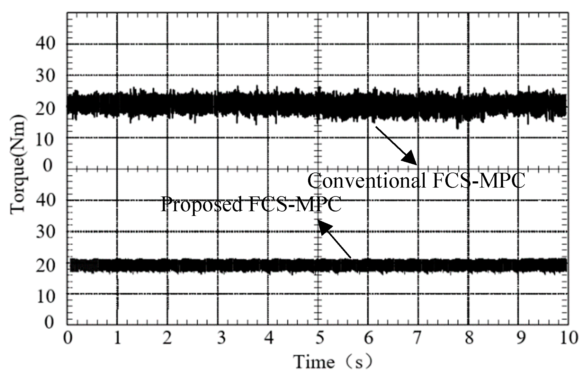
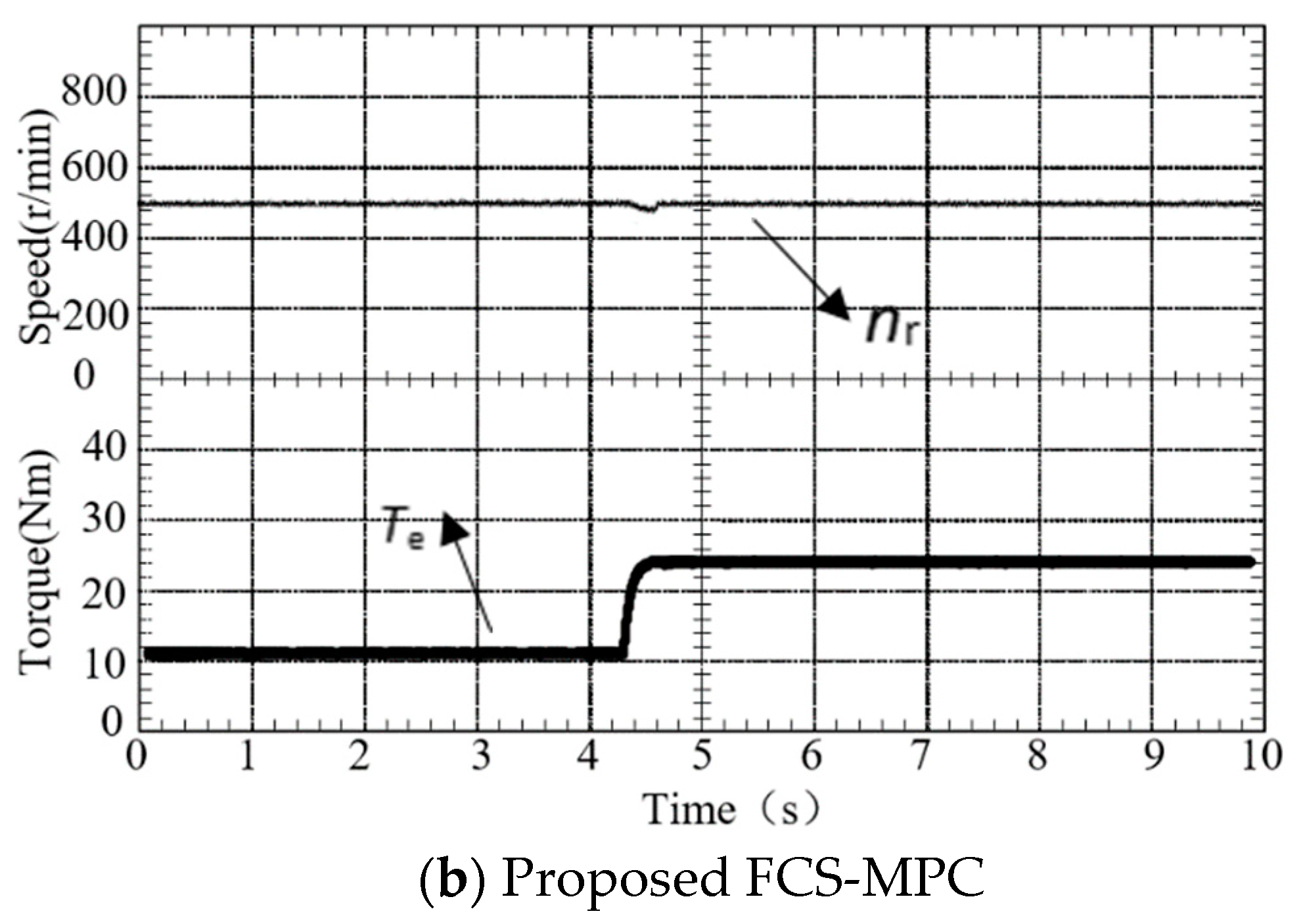
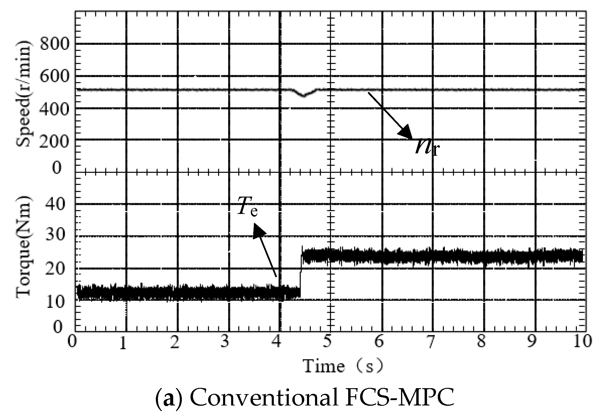
5. Experimental Test

The experiment aimed to verify the torque performance of this method with surface-mounted permanent magnet synchronous motor (SPMSM) and interior permanent magnet synchronous motor (IPMSM). The experimental platform as shown in Figure 10 was built by using dSPACE1102. The load of the PMSM is provided by the load machine.

5.1. Experiment on SPMSM

The parameters of the SPMSM are shown in Table 3. The steady-state performance test results of conventional FCS-MPC and proposed FCS-MPC are shown in Figure 11. In the experiment, the reference load torque was 20 N⋅m, and the results show that the proposed FCS-MPC significantly reduced the torque ripple under the same average switching frequency, while the conventional FCS-MPC had a lot of torque ripples (6 N⋅m) compared to proposed FCS-MPC (2.8 N⋅m). This is consistent with the simulation results.
In order to test the dynamic performance of the proposed FCS-MPC method, a load torque of 25 N⋅m was suddenly added when the steady speed of the motor was 500 rpm. Figure 12 shows that the response times of proposed FCS-MPC and conventional FCS-MPC are approximately the same; however, the proposed FCS-MPC strategy torque ripple is smaller than that of the conventional FCS-MPC. Meanwhile, the proposed FCS-MPC method enables the motor to quickly recover to the reference speed value compared to conventional FCS-MPC.

5.2. Experiment on IPMSM

Some parameters of the experiment motor are shown in Table 4. The following experiments were carried out in three aspects: torque steady-state responses, speed dynamics, and torque dynamics responses.
Figure 13 shows electromagnetic torque waveforms of two methods, with the load torque reference value set to 30 N⋅m. As can be seen from Figure 13, the method of proposed FCS-MPC can significantly reduce torque ripple by comparing torque waveforms; the average torque ripple of proposed method is only 3 N⋅m while that of conventional FCS-MPC is 7 N⋅m.
Figure 14 shows the waveforms of speed and electromagnetic torque of two methods when the starting moment of the motor and step change of load torque with load torque increasing from 10 to 20 N⋅m. It can be seen from Figure 14 that at the moment of starting the motor, the speed and electromagnetic torque of the conventional and proposed FCS-MPC methods increase sharply, reaching the given reference value quickly; however, compared with the conventional FCS-MPC, the strategy of proposed FCS-MPC has smaller torque ripple. When the load torque changes abruptly, the proposed FCS-MPC can also track the change of torque quickly, and the corresponding speed is faster than conventional FCS-MPC.
Through the analysis of the above experiments, compared with the conventional FCS-MPC control system, the proposed FCS-MPC in this paper effectively reduces the torque ripple and improves the following performance of the motor torque.

6. Summary

In this paper, a new scheme of direct torque control for PMSM based on a finite control set (FCS) model is proposed. The eight voltage vectors of the two-level converter are utilized as an FCS for the torque prediction of the PMSM. The cost function is used to estimate the duty cycle of each voltage vector. Thus, the optimal voltage vector can be obtained from eight voltage vectors and their duty cycles. Compared with the classical FCS-MPC method, the proposed method has smaller torque ripple and excellent dynamic performance.

Author Contributions

Conceptualization and methodology, G.B. and W.Q.; software, T.H.; validation, G.B. and W.Q.; writing—original draft preparation, T.H.; writing—review and editing, G.B. and W.Q.; funding acquisition, G.B. All authors have read and agreed to the published version of the manuscript.

Funding

This research was funded by supported by State Key Laboratory of Large Electric Drive System and Equipment Technology (SKLLDJJ032016018) and National Natural Science Foundation of China (51967012) and Scientific Research and Innovation Team Project of Gansu Education Department (2018C-09).

Conflicts of Interest

The authors declare no conflict of interest.

Appendix A

Proof of Lemma 1.
Finding partial derivatives of f ( i d , i q ) and T e = 1.5 p i q [ ψ f + ( L d L q ) i d ] based on current vectors i d and i q , respectively:
f ( i d , i q ) i d q = [ 1 + 2 ( L d L q ) ψ f i d , 2 ( L d L q ) ψ f i q ]
T e i d q = [ 1.5 p ( L d L q ) i q , 1.5 p ( ψ f + ( L d L q ) i q ) ]
Considering the torque T e as constant, the trajectory of the operating point moves along the direction of the α which fulfills ( T e / i d q ) α = 0 . The vector α can be described as:
α = ε [ 1.5 p ( ψ f + ( L d L q ) i q ) , 1.5 p ( L d L q ) i q ) ] T ,
where ε is a positive real number.
f ( i d , i q ) i d q α = 1.5 p ε [ ψ F + 3 ( L d L q ) i d ] 3 p ε ( L d L q ) 2 ψ f ( i d 2 + i q 2 ) < 0 .
Therefore, the function f ( i d , i q ) is a strict monotonic function along the constant torque curve. □
Proof of Lemma 2.
The Lyapunov function is derived as:
d V ( k + 1 ) d t = V ( k + 1 ) i d q k + 1 d i d q k + 1 d t .
Therefore, the trajectory of the current makes the value of Lyapunov function decrease and there exists a i d q k + 1 which fulfills:
V ( k + 1 ) d i d q k + 1 Δ i d q k + 1 0 .
Therefore, there exists a current derivative:
d i d q k + 1 d t = μ Δ i d q k + 1 ,
so that:
d V ( k + 1 ) d t = V ( k + 1 ) i d q k + 1 μ Δ i d q k + 1 0 .
Here, μ can be a very small positive constant. □
Proof of Lemma 3.
Any reference vector u d q * ( x ) within the region of feasibility [having a magnitude of less than ( 2 / 3 ) U d c ] is contained within one of the six nonzero switching sectors of width ( π / 3 ) with vertices ( v d 0 , v q 0 ) , ( v d i , v q i ) , and ( v d j , v q j ) , where i , j { 1 , , 6 } are the nonzero switching states to the left and right of the reference vector and ( v d 0 , v q 0 ) is one of the two zero vectors. Containment within a switching sector ensures the existence of coefficients γ and η satisfying γ , η 0 and γ + η 1 such that the reference vector is expressible as a convex combination of the realizable inputs, given by:
u d q * ( x ) = γ v d q i + η v d q j + ( 1 γ η ) v d q 0 .
Plugging Equation (A10) into Equation (21) and noting that the system is control affine, we see that [23]:
d V ( k + 1 ) d t = V ( k + 1 ) i d q k + 1 ( A i d q k + 1 + B u d q * + E ) = V ( k + 1 ) i d q k + 1 ( A i d q k + 1 + B ( γ v d q i + η v d q j + ( 1 γ η ) v d q 0 ) + E ) = γ V ( k + 1 ) i d q k + 1 ( A i d q k + 1 + B v d q i ) + η V ( k + 1 ) i d q k + 1 ( A i d q k + 1 + B v d q j ) + ( 1 γ η ) V ( k + 1 ) i d q k + 1 ( A i d q k + 1 + B v d q 0 ) + V ( k + 1 ) i d q k + 1 E
Because γ , η , and ( 1 γ η ) are all nonnegative, the following inequalities hold [12]:
{ V ( k + 1 ) i d q k + 1 ( A i d q k + 1 + B v d q i ) 0 V ( k + 1 ) i d q k + 1 ( A i d q k + 1 + B v d q j ) 0 V ( k + 1 ) i d q k + 1 ( A i d q k + 1 + B v d q 0 ) 0 ,
which completes the proof in Lemma 3. The theorem also guarantees the stability of the proposed control scheme. □

References

  1. Yang, J.F.; Hu, Y.W. Optimal direct torque control of permanent magnet synchronous motor. Proc. Chin. Soc. Electr. Eng. 2011, 31, 109–115. [Google Scholar]
  2. Depenbrock, M. Direct self-control (DSC) of inverter fed induction machine. IEEE Trans. Power Electron. 1988, 3, 420–429. [Google Scholar] [CrossRef]
  3. Uddin, M.N.; Zou, H.; Azevedo, F. Online loss-minimization-based adaptive flux observer for direct torque and flux control of PMSM drive. IEEE Trans. Ind. Appl. 2016, 52, 425–431. [Google Scholar] [CrossRef]
  4. Swierczynski, D.; Kazmierkowski, M.P. Direct torque control of permanent magnet synchronous motor (PMSM) using space vector modulation (DTC-SVM)-simulation and experimental results. In Proceedings of the Conference of the IEEE 2002 28th Annual Conference of the Industrial Electronics Society, Sevilla, Spain, 5–8 November 2002. [Google Scholar]
  5. Tang, L.; Zhong, L.; Rahman, M.; Hu, Y. A novel direct torque controlled interior permanent magnet synchronous machine drive with low ripple in flux and torque and fixed switching frequency. IEEE Trans. Power Electron. 2004, 19, 346–354. [Google Scholar] [CrossRef]
  6. Cho, Y.; Lee, K.B.; Song, J.H.; Lee, Y. Torque-ripple minimization and fast dynamic scheme for torque predictive control of permanent magnet synchronous motors. IEEE Trans. Power Electron. 2015, 30, 2182–2190. [Google Scholar] [CrossRef]
  7. Vafaie, M.H.; Dehkordi, B.M.; Moallem, P.; Kiyoumarsi, A. A new predictive direct torque control method for improving both steady-state and transient-state operations of the PMSM. IEEE Trans. Power Electron. 2016, 31, 3738–3753. [Google Scholar] [CrossRef]
  8. Zhang, Y.; Zhu, J. Direct torque control of permanent magnet synchronous motor with reduced torque ripple and commutation frequency. IEEE Trans. Power Electron. 2011, 26, 235–248. [Google Scholar] [CrossRef]
  9. Rodriguez, J.; Kazmierkowski, M.P.; Espinoza, J.R.; Zanchetta, P.; Abu-Rub, H.; Young, H.A.; Rojas, C.A. State of the art of finite control set model predictive control in power electronics. IEEE Trans. Ind. Inform. 2012, 9, 1003–1016. [Google Scholar] [CrossRef]
  10. Rodriguez, J.; Pontt, J.; Silva, C.; Salgado, M.; Rees, S.; Ammann, U.; Lezana, P.; Huerta, R.; Cortes, P. Predictive control of three-phase inverter. Electron. Lett. 2004, 40, 561–562. [Google Scholar] [CrossRef]
  11. Preindl, M.; Bolognani, S. Model predictive direct torque control with finite control set for PMSM drive systems, part 1: Maximum torque per ampere operation. IEEE Trans. Ind. Inform. 2013, 9, 1912–1921. [Google Scholar] [CrossRef]
  12. Liu, Q.; Hameyer, K. A finite control set model predictive direct torque control for the PMSM with MTPA operation and torque ripple minimization. In Proceedings of the 2015 IEEE International Electric Machines & Drives Conference (IEMDC), Coeur d’Alene, ID, USA, 10–13 May 2015; pp. 804–810. [Google Scholar]
  13. Geyer, T.; Papafotiou, G.; Morari, M. Model predictive direct torque control; part I: Concept, algorithm, and analysis. IEEE Trans. Ind. Electron. 2009, 56, 1894–1905. [Google Scholar] [CrossRef]
  14. Preindl, M.; Schaltz, E.; Thogersen, P. Switching frequency reduction using model predictive direct current control for high-power voltage source inverters. IEEE Trans. Ind. Electron. 2010, 58, 2826–2835. [Google Scholar] [CrossRef]
  15. Mayne, D.Q.; Rawlings, J.B.; Rao, C.V.; Scokaert, P.O.M. Constrained model predictive control: Stability and optimality. Automatica 2000, 36, 789–814. [Google Scholar] [CrossRef]
  16. Alam, K.S.; Akter, M.P.; Xiao, D.; Zhang, D.; Rahman, M.F. Asymptotically Stable Predictive Control of a Grid-Connected Converter Based on Discrete Space Vector Modulation. IEEE Trans. Ind. Inform. 2018, 15, 2775–2785. [Google Scholar] [CrossRef]
  17. Aguilera, R.P.; Quevedo, D.E. On stability and performance of finite control set MPC for power converters. In Proceedings of the Workshop Predictive Control Electrical Drives Power Electronics, Munich, Germany, 14–15 October 2011; pp. 55–62. [Google Scholar]
  18. Lee, J.S.; Lorenz, R.D.; Valenzuela, M.A. Time-optimal and loss minimizing deadbeat-direct torque and flux control for interior permanent magnet synchronous machines. IEEE Trans. Ind. Appl. 2014, 50, 1880–1890. [Google Scholar] [CrossRef]
  19. Xu, W.; Lorenz, R.D. Dynamic loss minimization using improved deadbeat-direct torque and flux control for interior permanent-magnet synchronous machines. IEEE Trans. Ind. Appl. 2014, 50, 1053–1065. [Google Scholar] [CrossRef]
  20. Chen, Y.; Sun, D.; Lin, B.; Ching, T.W.; Li, W. Dead-beat direct torque and flux control based on sliding-mode stator flux observer for PMSM in electric vehicles. In Proceedings of the 41st Annual Conference of the IEEE Industrial Electronics Society, Yokohama, Japan, 9–12 November 2015; pp. 2270–2275. [Google Scholar]
  21. Barcaro, M.; Fornasiero, E.; Bianchi, N.; Bolognani, S. Design procedure of IPM motor drive for railway traction. In Proceedings of the IEEE International Electric Machines & Drives Conference (IEMDC), Niagara Falls, ON, Canada, 15–18 May 2011; pp. 983–988. [Google Scholar]
  22. Bianchi, N.; Bolognani, S.; Ruzojcic, B. Design of a 1000 HP permanent magnet synchronous motor for ship propulsion. In Proceedings of the 13th European Conference on Power Electronics and Applications (EPE’09), Barcelona, Spain, 8–10 September 2009; pp. 1–8. [Google Scholar]
  23. Prior, G.; Krstic, M. Quantized-input control Lyapunov approach for permanent magnet synchronous motor drives. IEEE Trans. Control Syst. Technol. 2013, 21, 1784–1794. [Google Scholar] [CrossRef]
Figure 1. The main circuit of the permanent magnet synchronous motor (PMSM) drive.
Energies 13 00234 g001
Figure 2. Optimization process diagram of model predictive control (MPC).
Energies 13 00234 g002
Figure 3. Space vector analysis of the PMSM.
Energies 13 00234 g003
Figure 4. Stator current vector trajectory.
Energies 13 00234 g004
Figure 5. Block diagram of the proposed MPC.
Energies 13 00234 g005
Figure 6. Torque steady-state response simulation.
Energies 13 00234 g006
Figure 7. Torque dynamic simulation at t = 0.3 s.
Energies 13 00234 g007
Figure 8. Torque ripple simulation when the resistance is changed.
Energies 13 00234 g008
Figure 9. Torque ripple simulation when the flux is changed.
Energies 13 00234 g009
Figure 10. The controlled 6.5 kW PMSM drive test rig.
Energies 13 00234 g010
Figure 11. Torque steady-state responses (SPMSM).
Energies 13 00234 g011
Figure 12. Speed dynamic and torque dynamic responses (SPMSM).
Energies 13 00234 g012aEnergies 13 00234 g012b
Figure 13. Torque steady-state responses (IPMSM).
Energies 13 00234 g013
Figure 14. Speed dynamic and torque dynamic responses (IPMSM).
Energies 13 00234 g014
Table 1. Inverter switching states.
SaSbSc
0S1 on S4 offS3 on S6 offS2 on S5 off
1S1 off S4 onS3 off S6 onS2 off S5 on
Table 2. Switching state and voltage vector.
SaSbScVoltage Vector Uout
000 V 0 = 0
001 V 1 = 2 3 U d c e j 4 π 3
010 V 2 = 2 3 U d c e j 2 π 3
011 V 3 = 2 3 U d c e j π
100 V 4 = 2 3 U d c
101 V 5 = 2 3 U d c e j 5 π 3
110 V 6 = 2 3 U d c e j π 3
111 V 7 = 0
Table 3. Surface-mounted permanent magnet synchronous motor (SPMSM) parameters for simulation.
VariableParameterValue
P N Rated power6.5 kW
n N Rated speed1500 rpm
U N Rated voltage306 V
I N Rated current12.3 A
R Stator resistance1.01 Ω
L L d , L q 15 mH
p Number of pairs of poles4
J Rotary inertia0.01535 kg·m2
ψ f Flux linkage of the rotor0.175 Wb
Table 4. Interior permanent magnet synchronous motor (IPMSM) parameters for simulation.
VariableParameterValue
P N Rated power5.2 kW
n N Rated speed1500 rpm
U N Rated voltage380 V
R Stator resistance0.39 Ω
L L d 0.88 mH
L L q 1.62 mH
p Number of pairs of poles4
ψ f Flux linkage of the rotor0.163 Wb

