Dry Above Ground Biomass for a Soybean Crop Using an Empirical Model in Greece


Abstract
1. Introduction
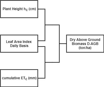
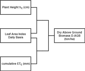
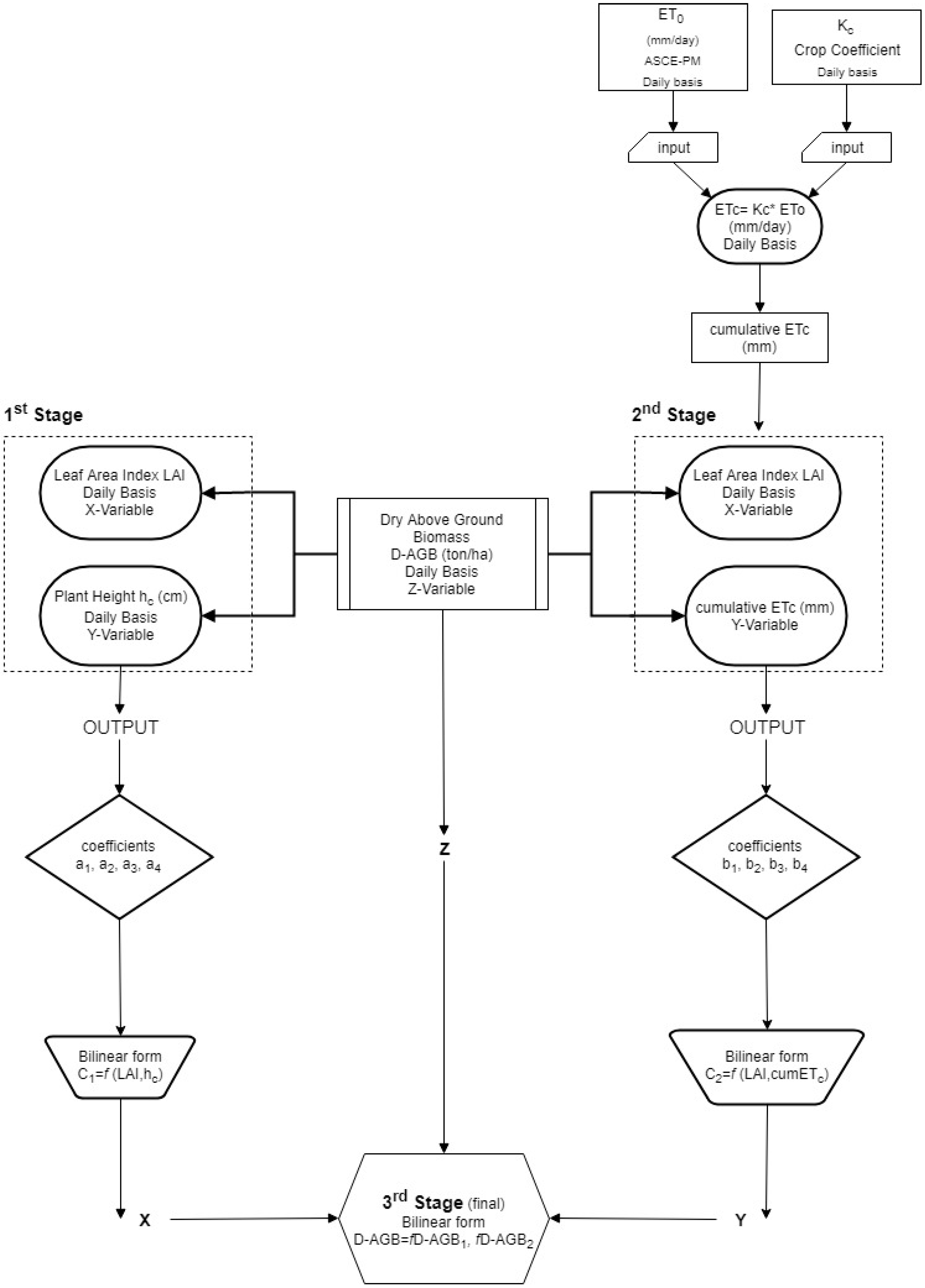
2. Methodology
- (1)
- Daily grass reference evapotranspiration as estimated by the FAO56 Penman-Monteith equation [18]. All the meteorological parameters used were collected from the automatic meteorological station of the laboratory of agricultural hydraulics, which is installed on a well-watered extended grass field, very close to the experimental plots (100 m). Meteorological data, such as air temperature (Tavg, Tmax, and Tmin), air relative humidity (RHavg, RHmean, RHmax), wind speed at the level 2 m (u2), solar radiation (Rs), net radiation (Rnet), photosynthetically active radiation sensor (PAR), and soil temperature (Tsoil), were collected. A rain gauge and wind direction sensor were also installed. All data were automatically collected and recorded from an acquisition system (data logger Campbell CR10X) in hourly and daily time step (averages).
- (2)
- Soil data as determined from the 1 m soil profile of the experimental field, which was characterized as clay (sand 21%, clay 60%, silt 19%), with a field capacity of 0.43 m3·m−3 and a wilting point of 0.15 m3·m−3.
- (3)
- The adjusted Kc values, which were Kc,ini: 0.47, Kc,mid: 1.10, and Kc,end: 0.50. The adjusted Kc values were estimated by using the single crop coefficient Kc method [18].
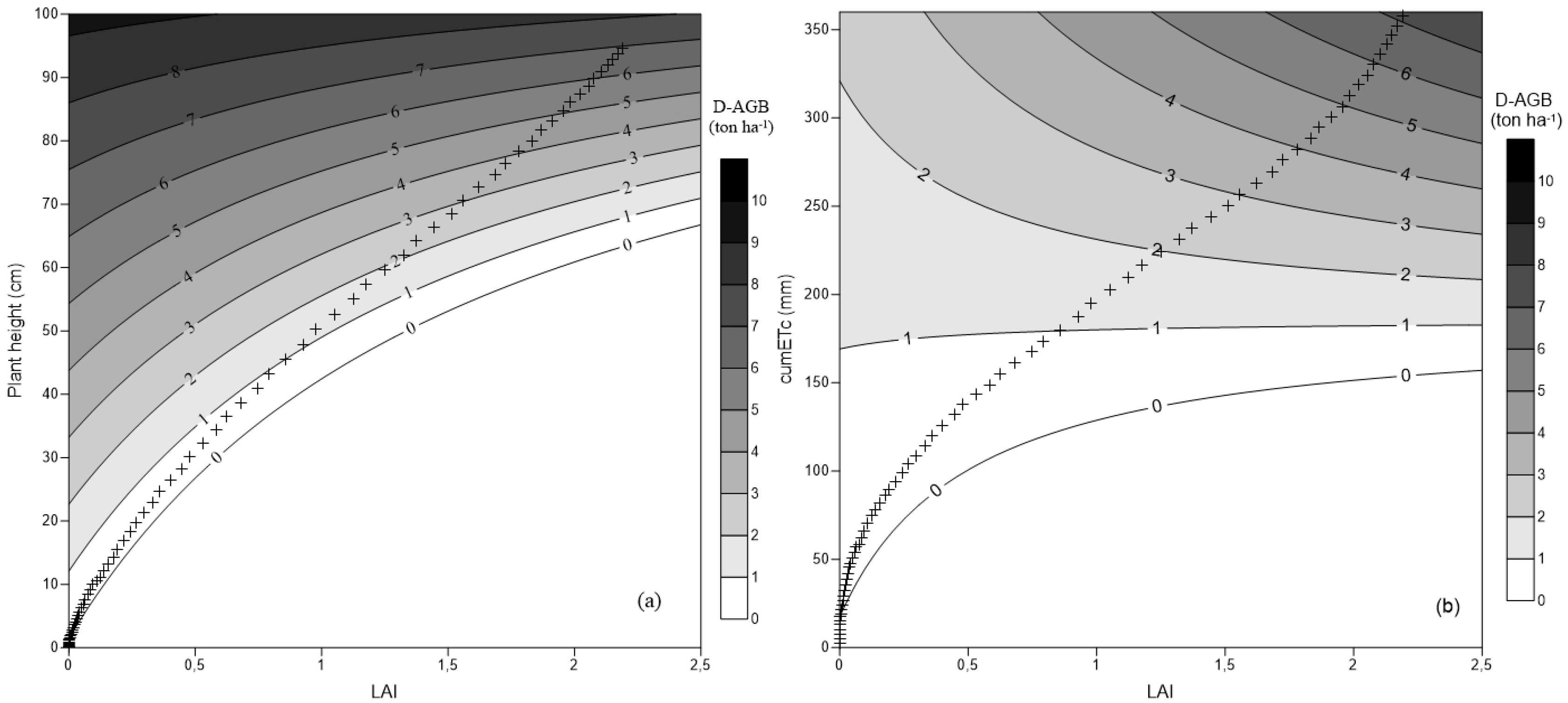
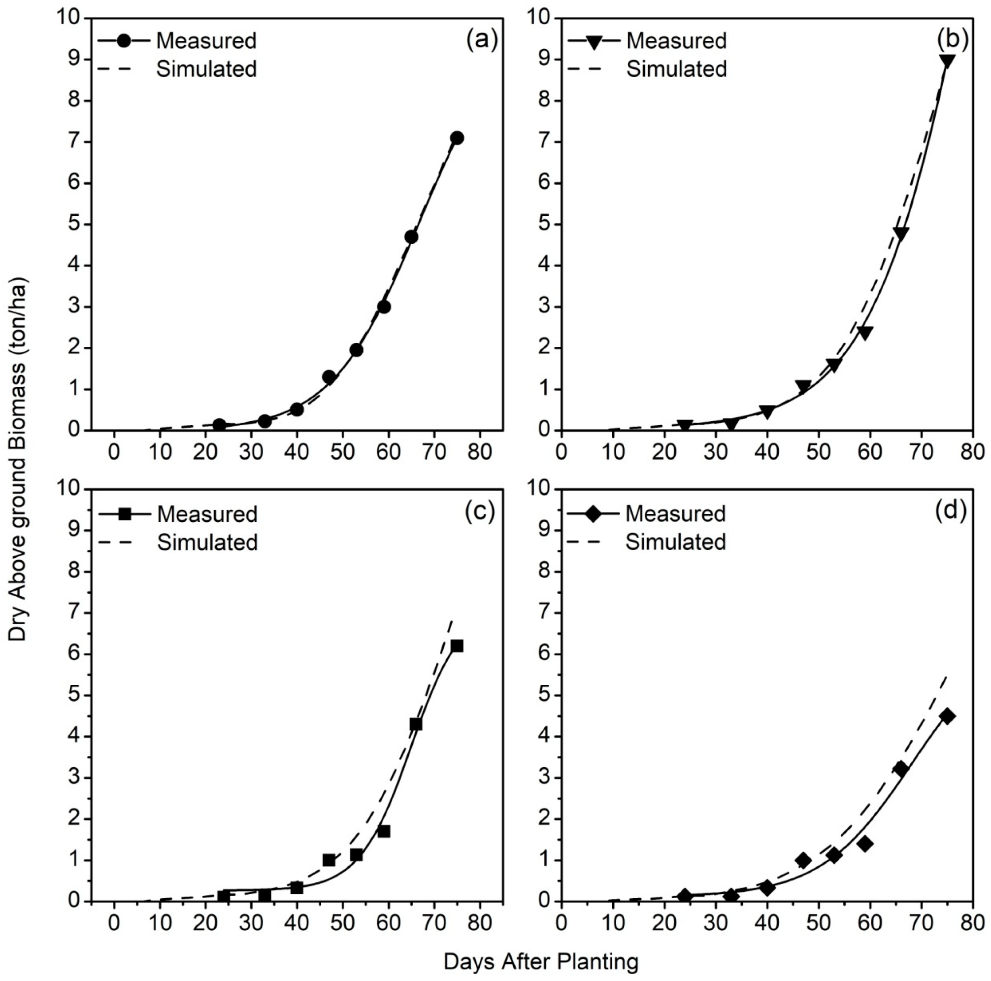
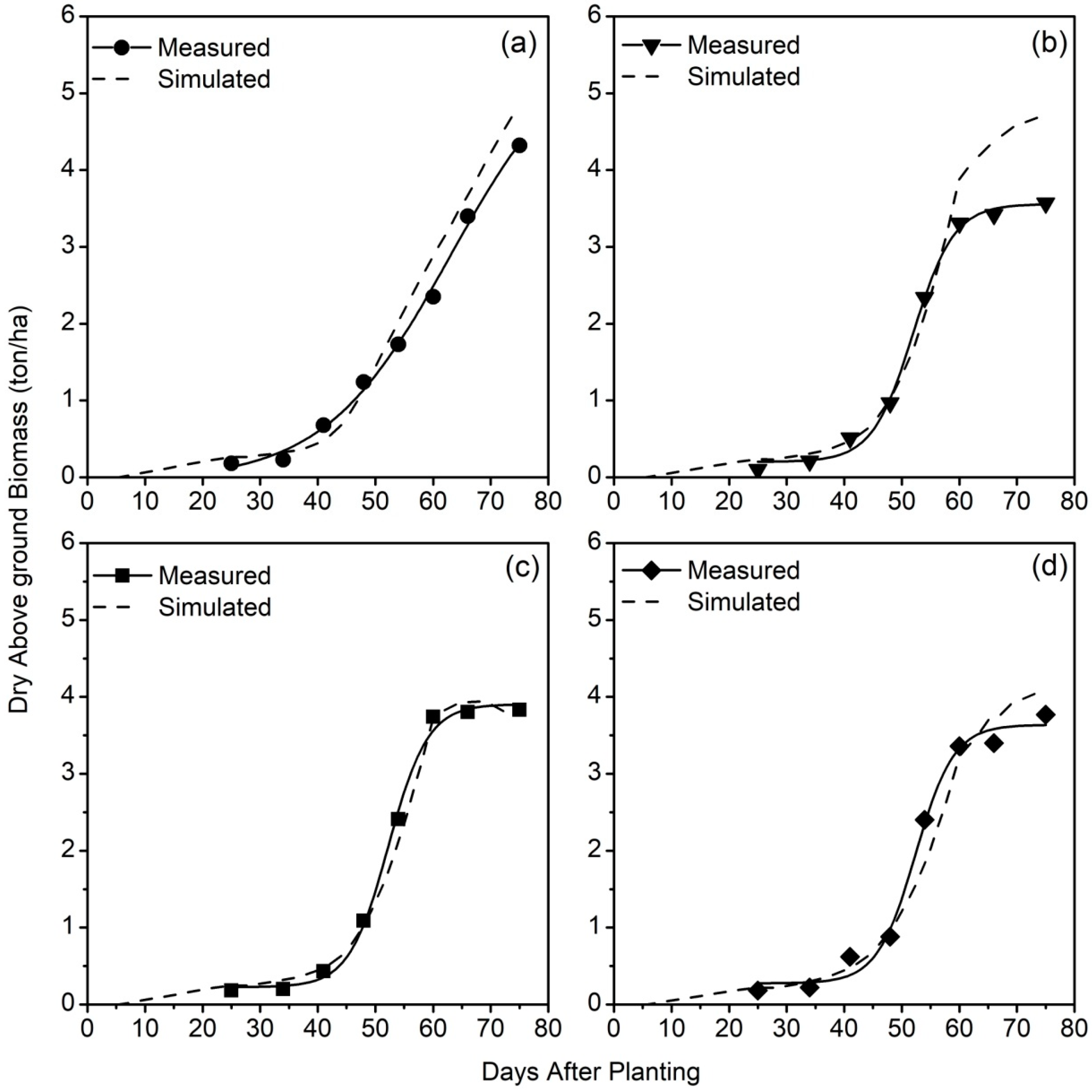
3. Results and Discussion
4. Conclusions
Author Contributions
Funding
Acknowledgments
Conflicts of Interest
References
- Madamba, S.P. The response surface methodology: An application to optimize dehydration operations of selected agricultural crops. LWT-Food Sci. Technol. 2002, 35, 584–592. [Google Scholar] [CrossRef]
- Sengo, I.; Gominho, J.; d’Orey, L.; Martins, M.; d’Almeida-Duarte, E.; Pereira, H.; Ferreira-Dias, S. Response surface modeling and optimization of biodiesel production from Cynara cardunculus oil. Eur. J. Lipid Sci. Technol. 2010, 112, 310–320. [Google Scholar] [CrossRef]
- Silva, G.F.; Castro, M.S.; Silva, J.S.; Mendes, J.S.; Ferreira, A.L.O. Simulation and optimization of biodiesel production by soybean oil transesterification in nonideal continuous stirred-tank reactor. Int. J. Chem. React. Eng. 2010, 8. [Google Scholar] [CrossRef]
- Tiwari, A.K.; Kumar, A.; Raheman, H. Biodiesel production from jatropha oil (Jatropha curcas) with high free fatty acids: An optimized process. Biomass Bioenergy 2007, 31, 569–575. [Google Scholar] [CrossRef]
- Vicente, G.; Coteron, A.; Martinez, M.; Aracil, J. Application of the factorial design of experiments and response surface methodology to optimize biodiesel production. Ind. Crops Prod. 1998, 8, 29–35. [Google Scholar] [CrossRef]
- Vicente, G.; Martınez, M.; Aracil, J. Integrated Biodiesel Production: A Comparison of Different Homogeneous Catalysts Systems. Bioresour. Technol. 2004, 92, 297–305. [Google Scholar] [CrossRef] [PubMed]
- Dalvi, V.B.; Tiwari, K.N.; Pawade, M.N.; Phirke, P.S. Response surface analysis of tomato production under microirrigation. Agric. Water Manag. 1999, 41, 11–19. [Google Scholar] [CrossRef]
- Photinam, R.; Moongngarm, A.; Paseephol, T. Process optimization to increase resistant starch in vermicelli prepared from mung bean and cowpea starch. Emir. J. Food Agric. 2016, 28, 449–458. [Google Scholar] [CrossRef]
- Formato, A.; Ianniello, D.; Villecco, F.; Lenza, T.L.L.; Guida, D. Design Optimization of the Plough Working Surface by Computerized Mathematical Model. Emir. J. Food Agric. 2017, 29, 36–44. [Google Scholar] [CrossRef]
- Muthuvelayudham, R.; Viruthagiri, T. Application of central composite design based response surface methodology in parameter optimization and on cellulase production using agricultural waste. Int. J. Chem. Biol. Eng. 2010, 3, 97–104. [Google Scholar]
- Pishgar-Komleh, S.H.; Keyhani, A.; Mostofi-Sarkari, M.R.; Jafari, A. Application of response surface methodology for optimization of picker-husker harvesting losses in corn seed. Iran. J. Energy Environ. 2012, 3, 134–142. [Google Scholar] [CrossRef]
- Alexandris, S.; Kerkides, P. New empirical formula for hourly estimations of reference evapotranspiration. Agric. Water Manag. 2003, 60, 181–198. [Google Scholar] [CrossRef]
- Alexandris, S.; Kerkides, P.; Liakatas, A. Daily reference evapotranspiration estimates by the “Copais” approach. Agric. Water Manag. 2006, 82, 371–386. [Google Scholar] [CrossRef]
- Poss, J.A.; Russell, W.B.; Shouse, P.J.; Austin, R.S.; Grattan, S.R.; Grieve, C.M.; Lieth, J.H.; Zeng, L. A volumetric lysimeter system (VLS): An alternative to weighing lysimeters for plant-water relations studies. Comput. Electron. Agric. 2004, 43, 55–68. [Google Scholar] [CrossRef]
- Meulenberg, C.J.W.; Vijverberg, H.P. Empirical relations predicting human and rat tissue: Air partition coefficients of volatile organic compounds. Toxicol. Appl. Pharmacol. 2000, 165, 206–216. [Google Scholar] [CrossRef] [PubMed]
- Wicki, A.; Parlow, E. Multiple Regression Analysis for Unmixing of Surface Temperature Data in an Urban Environment. Remote Sens. 2017, 9, 684. [Google Scholar] [CrossRef]
- Pereira, L.S.; Teodoro, P.R.; Rodrigues, P.N.; Teixeira, J.L. Irrigation scheduling simulation: The model ISAREG. In Tools for Drought Mitigation in Mediterranean Regions; Rossi, G., Cancelliere, A., Pereira, L.S., Oweis, T., Shatanawi, M., Zairi, A., Eds.; Kluwer: Dordrecht, The Netherlands, 2003; pp. 161–180. [Google Scholar]
- Allen, R.G.; Pereira, L.S.; Raes, D.; Smith, M. Crop Evapotranspiration, FAO Irrigation and Drainage Paper No 56; FAO: Rome, Italy, 1998; p. 327. [Google Scholar]
- Fox, M.S. An organizational view of distributed systems. IEEE Trans. Syst. Man Cybern. 1981, 11, 70–80. [Google Scholar] [CrossRef]
- Willmott, C.J. Some comments on the evaluation of model performance. Bull. Am. Meteorol. Soc. 1982, 63, 1309–1313. [Google Scholar] [CrossRef]


| Cross-Correlation/Covariance | LAI | hc | D-AGB |
|---|---|---|---|
| Variable correlation | |||
| LAI | 1.000 | 0.996 | 0.957 |
| hc | 0.996 | 1.000 | 0.935 |
| D-AGB | 0.957 | 0.935 | 1.000 |
| Variable covariance | |||
| LAI | 0.614 | 25.637 | 1.613 |
| hc | 25.637 | 1080.251 | 66.108 |
| D-AGB | 1.613 | 66.108 | 4.626 |
| Cross-Correlation/Covariance | LAI | cumETc | D-AGB |
|---|---|---|---|
| Variable correlation | |||
| LAI | 1.000 | 0.987 | 0.957 |
| cumETc | 0.987 | 1.000 | 0.929 |
| D-AGB | 0.957 | 0.929 | 1.000 |
| Variable covariance | |||
| LAI | 0.614 | 86.497 | 1.613 |
| cumETc | 86.497 | 12,505.448 | 223.44 |
| D-AGB | 1.613 | 223.44 | 4.626 |
| Treatments | Slope | MBE | RMSE | MAE | d | R2 | |
|---|---|---|---|---|---|---|---|
| 2015, (N = 75) | |||||||
| I75 | 1.113 | 0.239 | 0.450 | 0.262 | 0.640 | 0.998 | 0.986 |
| I50 | 1.073 | 0.315 | 0.498 | 0.371 | 1.010 | 0.996 | 0.966 |
| I25 | 1.347 | 0.446 | 0.678 | 0.490 | 1.990 | 0.988 | 0.978 |
| 2014, (N = 75) | |||||||
| I100 | 1.213 | 0.226 | 0.380 | 0.245 | 0.539 | 0.997 | 0.992 |
| I75 | 1.211 | 0.393 | 0.579 | 0.414 | 1.522 | 0.994 | 0.974 |
| I50 | 1.008 | 0.211 | 0.378 | 0.321 | 0.485 | 0.998 | 0.965 |
© 2020 by the authors. Licensee MDPI, Basel, Switzerland. This article is an open access article distributed under the terms and conditions of the Creative Commons Attribution (CC BY) license (http://creativecommons.org/licenses/by/4.0/).
Share and Cite
Vamvakoulas, C.; Alexandris, S.; Argyrokastritis, I. Dry Above Ground Biomass for a Soybean Crop Using an Empirical Model in Greece. Energies 2020, 13, 201. https://doi.org/10.3390/en13010201
Vamvakoulas C, Alexandris S, Argyrokastritis I. Dry Above Ground Biomass for a Soybean Crop Using an Empirical Model in Greece. Energies. 2020; 13(1):201. https://doi.org/10.3390/en13010201
Chicago/Turabian StyleVamvakoulas, Christos, Stavros Alexandris, and Ioannis Argyrokastritis. 2020. "Dry Above Ground Biomass for a Soybean Crop Using an Empirical Model in Greece" Energies 13, no. 1: 201. https://doi.org/10.3390/en13010201
APA StyleVamvakoulas, C., Alexandris, S., & Argyrokastritis, I. (2020). Dry Above Ground Biomass for a Soybean Crop Using an Empirical Model in Greece. Energies, 13(1), 201. https://doi.org/10.3390/en13010201