Abstract
Direct optical access to the combustion chamber of a gasoline direct injection (GDI) engine provides extremely valuable information about the combustion process. Experimental measurements of the geometric characteristics of the turbulent flame—such as the flame radius, flame center, flame edges and flame brush thickness—are of fundamental interest in support of the development and validation of any combustion model. To determine the macroscopic properties of sprays and flames, visualization and digital image processing techniques are typically used in controlled experimental setups like single-cylinder optical engines or closed vessels, while optical measurements on mass-production engines are more uncommon. In this paper the optical experimental setup (consisting of a high-speed camera, a laser light source and a data acquisition system) used to characterize the planar turbulent flame propagation in the cylinder of a 3.5 L GDI V6 mass-production engine, is described. The image acquisition process and the image processing that is necessary to evaluate the geometric characteristics of the propagating flame front, which are usually omitted in the referenced literature, are reported in detail to provide a useful guideline to other researchers. The results show that the step-by-step algorithm and the calculation formulae proposed allow to retrieve clear visualizations of the propagating flame front and measurements of its geometrical properties.
1. Introduction
Internal combustion engines represent the vast majority of the propulsion systems for ground transportation, thanks to the unrivaled power to weight ratio, fuel energy density, and short refueling time. Despite their first appearance dates more than one and a half century back, spark ignition engines are still the subject of research because some of the fundamental processes related to the combustion are not fully understood or explored yet [1,2]. On the other hand, the technology for the air-fuel mixture formation has faced substantial changes in the last decades. Gasoline direct injection (GDI) systems, which were first introduced in mass-production cars in the late 1990s, are now installed in more than 75% of the vehicles produced by eight of the largest manufacturers in the world, with several near or at 100% [3]. This technology gave the opportunity to develop stratified-charge and more advanced combustion modes [4,5,6,7]. At the same time, new low-carbon fuels have been synthesized and their combustion is subject to investigation [8,9,10]. Moreover, modeling, control, and optimization of the combustion process make room for further improvement of fuel economy, efficiency, and performance of the engine [11,12,13]. Finally, the increasing demand for reduced emissions represents an equally important driver for research into combustion. In this context, it is evident that experimental measurements play a major role in the understanding of the underlying processes and in support of the development and validation of any combustion model.
The analysis of the combustion process can be performed by means of in-cylinder pressure measurements together with visualization techniques based on high-speed imaging. While the in-cylinder pressure trace gives cycle-resolved information about the combustion process, the optical techniques represent a powerful tool for detailing the combustion process with high spatial and temporal resolution, allowing for a local analysis [14].
Aleiferis and Behringer [9] obtained planar laser-sheet visualizations of the flame front in a single-cylinder research engine. They processed the images with background subtraction, intensity equalization, filtering and binary conversion in order to identify the flame contour and calculate flame area, equivalent flame radius, roundness and center position.
Merola et al. [2], used an optically accessible single-cylinder GDI engine to perform optical diagnostics. Images were first converted into 256-grey scale and masking was applied. Then the contrast and brightness of the images were adjusted through a look-up table (LUT) transformation. An automatic interclass variance threshold method was applied starting from the light intensity histogram in order to obtain binary images. More details are provided by the same authors in a previous work [15].
Sementa et al. [16] used an endoscopic probe, installed in a protective case, to get optical access through a sapphire window into the combustion chamber of the 4th cylinder of a spark ignition direct injection, inline 4-cylinder, 4-stroke, 1750 cm3 displacement, turbocharged engine. Flame front contours were obtained by background subtraction and light intensity thresholding. The flame front center position and the distances of every point of the front from it along six different directions were calculated. The flame radius was obtained for every image by the average of the six distances.
Catapano et al. [10] performed the same image processing and calculations on a single-cylinder, 4-stroke, 250 cm3 displacement, GDI engine equipped with an elongated piston, a sapphire window and a quartz cylinder. In a more recent work [17], the same authors studied the behavior of gasoline-ethanol blends in a 4-cylinder, 1750 cm3, GDI engine. Two optical accesses were obtained for one of the cylinders: the first one with a sapphire window in the piston head, and the second one by means of an endoscopic probe inserted in the chamber through the engine head. Thus, this experimental setup required the design of elongated pistons and cylinders. Regarding the image processing, the background was detected in motored condition and then subtracted. Every 16-bit grey-scale image was converted in 12-bit grey-scale image. Convolution filtering and threshold segmentation were used to obtain binary images from which the flame could be detected and its radius could be calculated.
Bladh et al. [18] reported in more detail the procedure that they used to obtain flame propagation visualizations in a single-cylinder spark-ignition research engine using laser-induced fluorescence. The image processing steps were the following: background subtraction, laser profile compensation, image shift, binary image creation, contour recognition and, finally, velocity estimation.
Martinez et al. [19] studied the flame front propagation in an optical GDI engine under stoichiometric and lean burn conditions using cycle resolved digital imaging. The data was first exported as 8-bit grey-level images and pre-processed to adjust the contrast and brightness with respect to the maximum intensity value. Additionally, masking was applied to cut light from reflections at the boundaries of the optical access. Finally, a fixed threshold intensity value was applied to obtain binary images and detect the flame front position. The results of image processing consisted in the estimation of the flame area, the Waddel disk diameter, the circularity, and the flame center displacement.
Martinez-Boggio et al. [20] used an optically accessible SI single-cylinder engine with port fuel injection to investigate the effect of dilution on syngas combustion. The optical set-up allows a bottom view of around 78% of the piston diameter, and a lateral view of the entire cylinder diameter (82 mm) and half of the stroke (45 mm) in the vertical axis. The three main steps through which they processed the image data are shortly discussed in the paper: binarization, post-treatment, and flame outline identification. A set of four figures is presented to show the processing steps. The data was then used to estimate the flame area, the flame wrinkling (curvature), and the flame center displacement. Peñaranda et al. [21], used the same experimental setup and processed the images with a similar approach, but in their work they show the results of the processing steps for both the lateral and bottom views.
Disch et al. [22] aimed at visualizing the influence of engine parameters on individual consecutive combustion cycles during transient operation using optical diagnostics methods. The illumination access and the detection access are adapted in the cylinder head between the intake valves and exhaust valves of cylinder number 6 of an in-line, 6 cylinders, 2979 cm3, turbocharged, gasoline engine. They used an optical setup that has some common features to the one presented in this paper, however it had a different purpose.
In this work a 3.5 L GDI V6 mass-production spark ignition engine has been equipped with a camera and illumination system that allow direct optical access to one of the engine cylinders. The purpose of the experiments is to measure the flame front position with high spatial and temporal resolution. A calculation algorithm is proposed and equations are formulated in order to estimate the flame radius, flame center, flame edges, and flame brush thickness. Despite the effort of the authors in reviewing the literature to find more works related to the topic of processing turbulent flame propagation images in GDI engines, most of the referenced works only present a brief description of the image processing procedure, and point directly to the measurement results. Conversely, in this paper more emphasis is given to the description of the image processing steps that lead to the evaluation of the measurements of interest, which is usually the most time-consuming and tedious part of such kind of experimental activities. In the next section, the experimental setup is described, and a detailed flowchart for the digital image processing is presented. The explanation of each processing step and the motivation for each of them is considered as one of the valuable contributions from this paper. In the last section, results are shown that demonstrate the application of the image processing flowchart to collected image data. Qualitative visualizations of the turbulent flame propagation are presented, and the results of the calculations of the flame center, flame radius, and flame edges are reported in the form of processed images for three consecutive cycles.
2. Experimental Setup and Methods
The engine test cell is shown in Figure 1, in which the main components of the experimental setup can be identified: the engine, the dynamometer and the optical hardware (the high speed camera and its support structure, the lens and the endoscope; the laser arm, endoscope and control unit; the oil seeding system). Every component is described in more detail in the next subsections. The characteristics of the main sensors and of the data acquisition system are also illustrated.
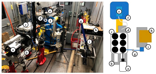
Figure 1.
Picture (left) and schematic (right) of the engine test cell and experimental setup: (a) high speed camera; (b) camera support frame; (c) engine; (d) air box; (e) particle seeder; (f) AC dyno; (g) articulated guide arm; (h) laser controller; (i) laser.
2.1. Engine
A 3.5L GDI V6 mass-production spark ignition engine, whose main parameters are reported in Table 1, has been mounted on a test bench.

Table 1.
Engine parameters.
Each cylinder has 4 valves and one GDI 6 holes injector. The injection system can deliver pressures up to 20 MPa of the indolene test fuel. The engine head has been machined to realize two perpendicular holes through the combustion chamber of the cylinder of the front bank on the timing belt side. A removable protective case with a sapphire window has been fastened in each hole to accommodate the optical access for the endoscopes. A crank pulley mounted crank angle encoder with an accuracy of 0.25 degrees has been adopted to measure the engine speed. The in-cylinder pressure is measured with an indicating sparkplug pressure transducer. Thermocouples, mass flow meters, and oxygen sensors have also been installed. High speed data acquisition is sampled at up to 100 Hz. The engine is connected to a four-quadrant 300 HP alternating current dynamometer, as shown in the picture in Figure 1. The control interface of the dynamometer allows to set the engine speed in RPM or the engine load.
2.2. Optical Hardware
Key-hole imaging using endoscopes is a minimally invasive technique to monitor real-time in-cylinder processes in real engines. The optical chamber measurement layout is designed to capture planar images of the turbulent flame front that propagates in time and space, from the spark plug towards the cylinder walls. Therefore, the two windows, that provide the access inside the cylinder to the light source and the camera, have been machined in two perpendicular directions that point towards the spark plug. To ensure high spatial and temporal resolution of the flame front propagation (typically 1 image/CAD (crank angle degree)), a phantom ultra-high-speed v1612 camera has been employed. It is capable of capturing 16 Giga-pixels per second of data from a 1 Mega-pixel, 12 bit, CMOS sensor with 28 µm pixel size. At full resolution of 1280 × 800, the camera can achieve throughput of 16 giga-pixels per second with a maximum frame rate of 16,000 frames per second. A Nikon Nikkor 105 mm lens is mounted to the camera with wide open diaphragm. A 527 nm band-pass filter was used to isolate only the geometric scattered light from the laser. Table 2 summarizes the parameters of the camera.
Table 2.
Camera parameters.
A very short exposure time (which must be shorter than the time interval between two subsequent frames) requires a very powerful and high-speed source of light, as recommended in [23]. Thus, a class IV laser, model DM30-527DH by Photonic Industries, has been used. As reported in Table 3, it is a double beam diode pumped Nd:YLF laser with a pulse repetition rate to 10 kHz, wavelengths of 1053 and 527 nm and maximum energy per pulse of 70 mJ. Timing of the engine operation with the camera and the laser is controlled by LaVision’s triggering and synchronization unit PTU X and the software platform DaVis [24]. Considering that 1 video recording can require up to 100 GB of memory to be stored, two hard drives have been employed: a 300 GB SSD and a 10 GB network card that allows up to 600 MB/sec download speeds.
Table 3.
Laser parameters.
A specifically designed frame has been mounted to the engine to support the camera (see Figure 1), while the laser beam is guided through an articulated arm toward the combustion chamber of the optical cylinder. Two endoscopes are inserted in the two windows machined in the cylinder head, one for the camera and the other for the laser. The laser endoscope contains a biconcave cylindrical lens from Laser Component GmbH that produces 60° diverging planar light sheet from a 3–7 mm diameter collimated beam. The final layout of the optical measurement setup is depicted in the scheme in Figure 2.
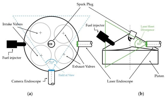
Figure 2.
Optical measurement setup layout: (a) top view; (b) side view.
As it is shown, the laser and the camera are placed at an angle of 90° relative to each other. The camera points at the spark plug, and its field of view covers an angle of approximately 70°, with the intake valves on the left side and the exhaust valves on the right side. The laser light enters as a point source from the right side of the field of view, and it spreads into the cylinder with a 60° divergence, creating a sheet that illuminates the axial plane of the cylinder that passes between each set of valves and through the spark plug. The fuel injector is placed on the left side of the field of view and it directly sprays the indolene into the cylinder.
In order to obtain planar visualizations of the flame front with a clear separation between the burned and unburned regions, seeding particles that scatter the laser light are injected in the intake of the engine through a tube connected to the seeder (see Figure 1). The seeding particles are then ingested into the cylinder together with the air during the intake stroke, while the fuel is directly injected into the cylinder. The seeding system consists of an atomizer that is able to generate particles of different sizes depending on the injection pressure. Tests have been performed in order to determine the most appropriate pressure for every engine operating condition. Since the engine is naturally aspirated, the seeding particles are injected in the intake system just downstream of the air-box filter. Vegetable oils have been chosen for seeding because they burn together with the mixture, leaving a dark region behind the flame front (no particles will be present in the burned region, hence no light is scattered to the camera) and a bright region in front of it, where the oil particles are still present and scatter the light to the camera. Several readily available and inexpensive oils have been tested: soy-bean oil, olive oil, and Crambe abyssinica oil, among others. These vegetable oils are composed of a mixture of many chemicals, including triglycerides, which are complex molecules with a high molecular weight, which provides a high boiling point. Their main properties are reported in Table 4, which shows the positive correlation between molecular weight and boiling point temperature.
Table 4.
Oils properties [25,26].
After testing the different oils, Crambe abyssinica has been eventually selected because of its high boiling point, which allows the oil particles in the unburned region to survive longer and only burn when reached by the flame front. Therefore, the recorded images showed the highest and most durable separation between the burned and unburned regions inside the combustion chamber. The amount of oil is very dilute compared to the fuel, but which has not been directly measured because only the pressure of the seeder valve can be measured. However, considering that all the tests required 24.1 kg of indolene and only 0.175 kg of vegetable oil, it can be estimated that the oil to fuel ratio is approximately 0.0073.
2.3. Digital Image Processing Flowchart
Once the optical hardware settings are done (laser light pulse intensity, camera frames per second, lenses adjustments), an experimental campaign can be carried out and videos can be acquired for different engine operating conditions (speed and load). Every video is recorded with a duration which corresponds to a desired number of engine cycles. For every cycle, a number of images is recorded which corresponds to a desired crank angle resolution (1 or 2 CAD). Based on the engine speed in RPM, the number of cycles is simply given by Equation (1), while the number of camera frames per second (fps) required for a desired crank angle resolution (CADres) is calculated from Equation (2):
The number of acquired images will just be given by the product of the fps and the recorded seconds. After the data acquisition, four main activities have been identified which lead to the measurement of the turbulent flame properties of interest (flame center, flame radius, and flame brush thickness):
- Pre-processing;
- Image binarization;
- Flame edges detection;
- Post-processing.
The activities in the above list must be repeated for each one of the acquired images. In the following subsections, each activity is motivated and discussed, while an overall detailed flowchart is presented in Figure 3.
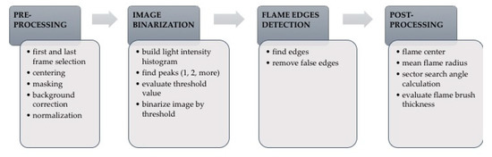
Figure 3.
Image processing flowchart.
2.3.1. Pre-Processing
Before starting the actual processing, the image files must pass through a series of pre-processing steps that aim at removing noise and preparing the image for the next processes. In addition, given the tremendous amount of data, a preliminary step requires to select the first and the last useful images for every cycle and cut away the remaining unnecessary frames. For the purpose of this investigation, the first frame in which the flame is visually detectable by human observation is taken as the first useful image, while the last frame is taken when the flame has reached the periphery of the field of view. In addition, masking is required because the camera records not only the region of interest, but also reflected light from the cylinder walls, chamber roof, valves, spark plug, and moving piston. These uninteresting features can be removed by a mask.
The optics of the endoscope requires the camera to be mounted approximately 410 mm from the optical cylinder. This separation distance between the camera and engine mass, and the non-rigid mounting structure cause undesired relative motion of the camera endoscope with respect to the optical access window. In order to remove the camera shake, a reference region can be selected, e.g., the spark plug electrodes, and all the images (for every crank angle and for every cycle) can be centered with respect to that region. In particular, a 64 × 64 pixel window is drawn around the spark plug in the first frame. The pixels in this window have a very strong light intensity due to the light reflections on the electrodes, thus resulting in strong reference signal for centering each frame via cross-correlation.
The flame front detection algorithms are usually based on threshold techniques that enable to distinguish the bright regions of fresh mixture from the dark regions of burned gases. Therefore, it is very important that inside the observation region (the combustion chamber) the light intensity is evenly distributed. High quality thresholding requires addressing the light divergence, which necessarily decreases the light intensity as a function of the distance from the source. Figure 2 shows that the laser enters into the cylinder from a point source on the right hand side and spreads into the chamber with a 60° divergence, forming a planar sheet. Hence, along the path to reach the opposite cylinder wall, the light intensity is decreasing as it propagates away from the source. As a consequence, the light intensity of a raw image along a fixed coordinate appears uneven: the intensity values are clearly unbalanced both in the x and y directions, and attain highest values close to the point where the light source enters on the right side. Such an intensity distribution makes robust threshold segmentation difficult. Therefore, background intensity correction and normalization are performed to obtain a more even distribution of the light intensity across the region of interest, along both the x and y axes, and remove the correlation between high values of intensity and low values of distance from the source. The correction is obtained by increasing the values of intensity with a multiplier that is a function of the distance of every pixel from the light source: the higher the distance , the smaller the multiplier :
where is half of the width of the diverging laser sheet at distance and is half of the width of the light as it exits the endoscope, while the exponent is a tunable parameter.
The normalization is then obtained by dividing the corrected light intensity of every frame by the corrected light intensity of a frame in which the ignition has not begun yet, which is taken as a reference. The result of these pre-processing steps is an image with a more even distribution of the light intensity.
2.3.2. Image Binarization
The pre-processed images are now suitable for identifying a threshold value of light intensity which allows to distinguish the bright regions of fresh mixture from the dark regions of burned gases. Once the appropriate threshold value has been found, the image can be converted into a binary file, where every pixel is associated a value of 0 or 1. In such an image, the flame front can be easily identified at the interface of 0 and 1 values. However, the choice of the threshold is somewhat arbitrary and must be as accurate and robust as possible. The procedure used for finding the appropriate threshold, frame by frame, is described below.
The first step to determine the threshold value is to build a histogram of the light intensity for every image: the corrected light intensity range is divided into bins, and the number of pixels with an intensity value that falls into each bin is counted. The bin size is adjusted until a unimodal or bimodal histogram shape can be identified.
The second step is to study the shape of the histogram. If only a single peak is identified, that means there is not a clear separation in the number of bright and dark pixels, hence the combustion has either not started yet, or is already complete. On the other hand, if the histogram has two peaks, this is evidence that a clear separation shows up between bright unburned and dark burned regions, hence the combustion process has started.
The last step consists in determining a single light intensity value that best separates the bright region from the dark region. The choice made in this work is to consider the threshold value as the mean value of the intensities of the two peaks.
Once the threshold value has been determined, the image binarization can be performed: every pixel with an intensity that is higher than the threshold will be associated a value of one, while those pixels with an intensity lower than the threshold will be given a value of zero.
2.3.3. Flame Edges Detection
The binarized image is simply a matrix of zeros and ones, in which the flame front is located at the interface between zeros and ones. To locate the interface, a 3 × 3 pixel moving window is used to scan all the pixels and create a new matrix whose elements are the maximum value found in every window. In this way the unburned gas region (made of ones) is virtually augmented by an extra layer of ones. If now the new matrix of maxima is subtracted to the original matrix, a third matrix is obtained, whose elements are zeros everywhere except at the interface that is thus detected. Nonetheless, particular care must be taken in three situations:
- The flame is close to the boundaries of the region of interest;
- The flame propagates with large wrinkles;
- The flame is detected in very small regions away from the front.
In the first case, part of the domain boundary could be erroneously be accounted for as part of the flame front. In the second case, because of the configuration of the optical setup (which produces an axial view), the largest wrinkles could appear as detached from the flame front (see Figure 4) and be excluded from the computation. In the last case, residual noise can result in some areas (smaller than 3 × 3 pixels) to be considered as part of the flame front, even though they are actually noise far away from the flame front. Therefore, the algorithm for the edge detection must exclude those regions which are too close to the domain boundaries and those that are small and isolated, while it must include the apparently detached flames. Note that the second requirement is already satisfied by the filtering effect of the 3 × 3 pixel moving window calculation for the matrix of maxima.
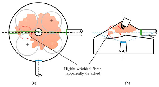
Figure 4.
Highly wrinkled apparently detached flames: (a) top view; (b) side view.
2.3.4. Post-Processing
The flame center, flame radius, and flame brush thickness are eventually calculated in the post-processing phase for every frame, according to the scheme reported in Figure 5.
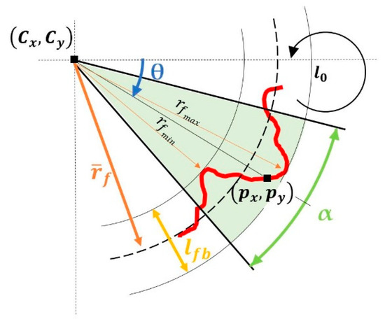
Figure 5.
Geometric characteristics of the turbulent flame front.
The flame center is evaluated as the geometric centroid of the pixels of coordinates that belong to the flame front edges, therefore its coordinates are simply calculated as:
The mean flame radius can then be calculated as the average value of the distance of every pixel that belongs to the flame front from the center:
In addition, the minimum and the maximum radii can be recorded.
For the calculation of the flame brush thickness, some additional calculations are required. The angular coordinate of every pixel on the flame front is evaluated clockwise from the horizontal:
Then, the flame front is divided into search sectors of amplitude , as a function of the integral length scale of the turbulence (typically 1–4 mm [27]):
For every pixel the surrounding angular interval is considered, and inside that interval the maximum and minimum radii are calculated. Thus, the flame brush thickness for the search sector related to the pixel is calculated as:
Finally, the average flame brush thickness is calculated as the average of the flame brush thicknesses evaluated for every pixel of the flame front:
3. Results and Discussion
The flowchart presented in the previous section is now applied to analyze the data collected for one engine operating point, namely wide-open throttle at 1000 RPM. The operating conditions of the engine and the main settings of the camera and laser are reported in Table 5. The “pre-processing” and “binarization” steps are only illustrated for one frame, while the “flame edges detection” is shown for 8 frames of the same cycle. Finally, processed images are presented for three consecutive engine cycles to prove that the algorithm is able to detect the flame edges, and to show how the turbulent propagation results in very different flame behaviors even for the same engine operating conditions, contributing to the cycle-to-cycle variability of the engine performance.
Table 5.
Experimental settings for the presented results.
3.1. Pre-Processing
A raw image, with the piston at TDC and the combustion taking place, is reported in Figure 6a to demonstrate the necessity of the pre-processing, in particular of the background correction. The light intensity along the x axis is plotted for three y coordinates. It is clearly shown that the distribution of the light intensity is unbalanced: most of the pixels close to the light source are extremely bright, while the other ones are much darker. At the same time, along the y coordinate the distribution is uneven, as it is shown by the different heights of the three curves.
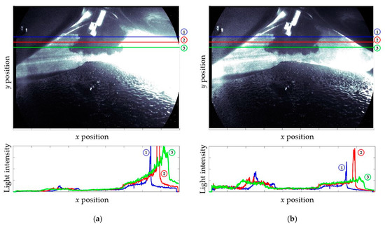
Figure 6.
Light intensity plots: (a) raw image; (b) background corrected image.
The background correction described in Section 2 is then applied, and the resulting image is reported in Figure 6b. The light intensity is plotted for the same three y coordinates of Figure 6a. Comparing Figure 6a,b, it can be observed that the pre-processed image presents a much more even distribution of the light intensity, both in the x and y directions. The difference can even be appreciated just by visually comparing the two images. In particular, it can be noted how the correction multiplier is effective in reducing the high intensities near the light source, as prescribed by Equation (3).
For the sake of completeness, the layers used to mask out the cylinder walls, chamber roof, moving piston, sparkplug and its shadow are shown in Figure 7. The only region that is left is the combustion chamber.
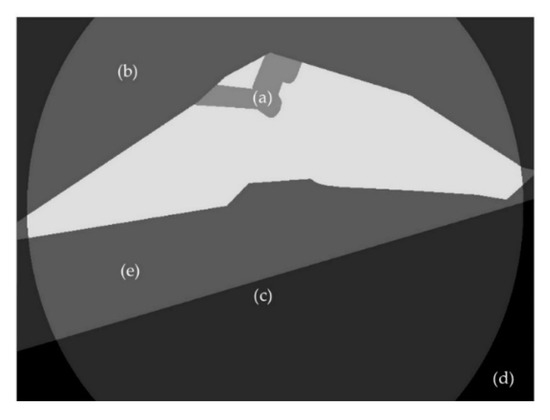
Figure 7.
Mask layers: (a) spark plug and shadow; (b) cylinder head and valves; (c) light sheet limit; (d) endoscope field of view; (e) piston.
3.2. Image Binarization
Once that every frame of the cycle has been corrected, light intensity histograms can be built as described in Section 2.3.2 in order to identify the threshold value of light intensity by which the image can be binarized. Figure 8 presents the histogram obtained from the same background corrected frame reported in Figure 6b.
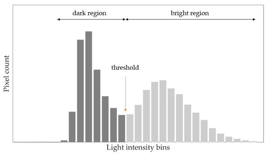
Figure 8.
Light intensity histogram.
Since the histogram is bimodal, the algorithm knows that the combustion has started and calculates the threshold value by which binarizes the image. The resulting binarized image is reported in Figure 9. This image is just a matrix composed of white pixels (with a value of one) in the burned region, and black pixels (with a value of zero) in the unburned and masked regions. The flame front can already be visualized at the interface between black and white pixels.

Figure 9.
Binarized image: the image is a matrix of ones (white) and zeros (black). The flame front is located at the interface.
3.3. Flame Edges Detection
The pre-processing and the binarization can be applied to all the frames, and after that the moving window technique discussed in Section 2.3.3 can be used to obtain clear visualizations of the flame front and its propagation. For instance, Figure 10 shows at steps of 2 CAD the flame edges from −4 to +10 CAD with respect to TDC.

Figure 10.
Flame edges detected for 1000 RPM @ 730mmHg (−4 to +10 CAD with respect to TDC). CAD: crank angle degrees; TDC: top dead center.
3.4. Post-Processing
Finally, the post-processing calculations are performed, and the results are visually presented in the following pages (see Figure 11, Figure 12, Figure 13, Figure 14, Figure 15 and Figure 16). The frames corresponding to crank angles −7 to 8 with respect to the firing top dead center position are shown for three consecutive cycles. The flame edges are represented with thick red lines; the flame center is recognized by a yellow star marker; the maximum and minimum mean flame front radii are identified by the circular solid red lines; the average radius of the flame front is drawn as a dashed red line in between the maximum and minimum radii. All these quantities are superimposed to the corresponding background corrected images in order to give an immediate feedback about the quality of the algorithm. It can be noted that, despite the complexity of the flame front geometry, the algorithm is able to accurately detect the flame edges and, consequently, to evaluate the geometric properties.
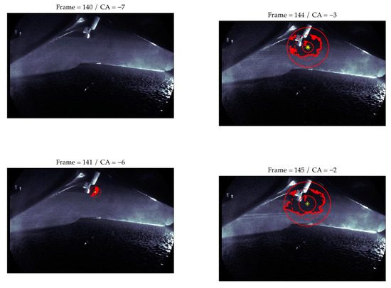
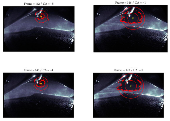
Figure 11.
Cycle 58. Background corrected images of turbulent flame from −7 CAD to TDC firing. Superimposed geometric properties: flame edges, flame center, min, max, and average radii. Engine operation: 1000 RPM, wide open throttle.
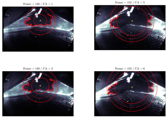
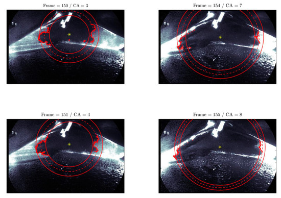
Figure 12.
Cycle 58. Background corrected images of turbulent flame from 1 to 8 CAD after TDC firing. Superimposed geometric properties: flame edges, flame center, min, max, and average radii. Engine operation: 1000 RPM, wide open throttle.
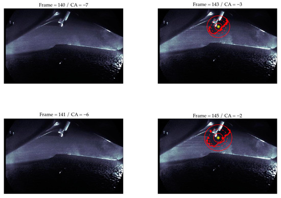
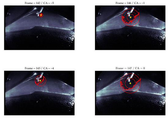
Figure 13.
Cycle 59. Background corrected images of turbulent flame from −7 CAD to TDC firing. Superimposed geometric properties: flame edges, flame center, min, max, and average radii. Engine operation: 1000 RPM, wide open throttle.
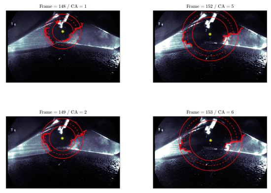
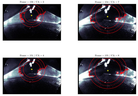
Figure 14.
Cycle 59. Background corrected images of turbulent flame from 1 to 8 CAD after TDC firing. Superimposed geometric properties: flame edges, flame center, min, max, and average radii. Engine operation: 1000 RPM, wide open throttle.
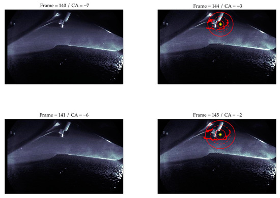
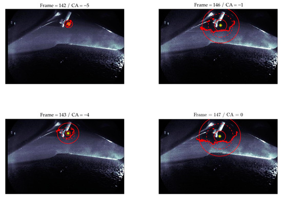
Figure 15.
Cycle 60. Background corrected images of turbulent flame from −7 CAD to TDC firing. Superimposed geometric properties: flame edges, flame center, min, max, and average radii. Engine operation: 1000 RPM, wide open throttle.
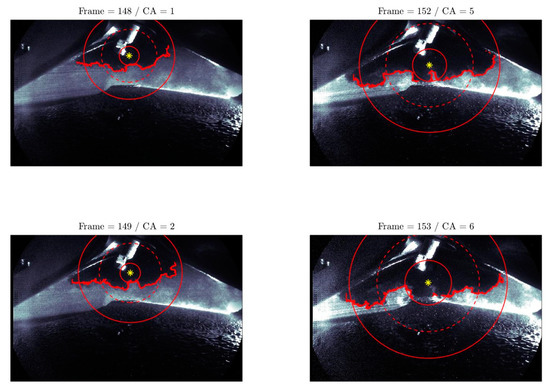
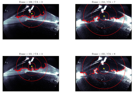
Figure 16.
Cycle 60. Background corrected images of turbulent flame from 1 to 8 CAD after TDC firing. Superimposed geometric properties: flame edges, flame center, min, max, and average radii. Engine operation: 1000 RPM, wide open throttle.
The first thing that can be observed is that for cycles 59 and 60 the flame front only becomes visible at −5 CAD before TDC, while in cycle 58 it is already visible at −6 CAD. Despite the different start, in every case the flame front has not reached the piston when it is at TDC. In cycle 60 the flame propagates mostly in the radial direction, and assumes a very stretched and wrinkled shape. It is remarkable that the processing algorithm is able to detect the flame edges even is such a condition where portions of unburned mixture are incorporated by the burned gases, see for example frames 154 and 155 in Figure 16. In cycle 60, because of the predominant radial propagation, the flame only reaches the piston at 5 CAD after TDC, while in cycle 58 and 59 this happens at 2 and 1 CAD after TDC, respectively. Another behavior that can be visually recognized is the thickening of the flame brush (represented by the distance between the maximum and minimum flame radii) during the turbulent propagation, which is common to all the 3 cycles. On the other hand, the behavior of the flame brush thickness when it is approaching the cylinder walls is different in the three cases: in cycle 58 it clearly starts to decrease, in cycle 59 it stay almost constant, and in cycle 60 it actually reaches the maximum value. Obviously, this is related to the increased level of flame wrinkling that is observed for cycle 60.
Even though Figure 11, Figure 12, Figure 13, Figure 14, Figure 15 and Figure 16 clearly demonstrate the calculations performed by the algorithm, the flame fronts for the three cycles can also be collected as is shown in the plots of Figure 17. This allows for a more straightforward comparison between the three cycles. Flame fronts are presented from −4 to +10 CAD with respect to TDC, with steps of 2 CAD. Figure 17 allows to retrieve additional information about the different directions and speeds of the propagating flames. For instance, it can be qualitatively assessed that the flame in cycle 58 (Figure 17a) propagates evenly in both the axial and radial directions, while the propagation in cycle 59 (Figure 17b) appears to prefer the axial direction, and in cycle 60 (Figure 17c) the radial direction is preferred. In addition, the flame front of cycle 59 (Figure 17b) appears to be the fastest one in reaching the piston, while cycle 58 (Figure 17c) is the slowest in approaching the cylinder walls, since at +10 CAD it appears to be the farthest from the walls.
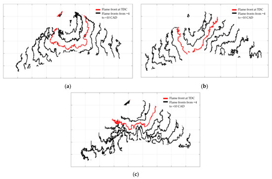
Figure 17.
Flame front propagation in three consecutive engine cycles at 1000 RPM, wide open throttle: (a) cycle 58; (b) cycle 59; (c) cycle 60.
4. Conclusions
In the present work the geometric properties of a propagating turbulent flame have been measured in a 3.5L GDI V6 mass-production engine. Slight modifications to the cylinder head have been made in order to provide optical access to the combustion chamber. Two perpendicular holes have been machined to seat two endoscopes: one for the optics and one for the laser illumination. All the requirements for high spatial and temporal resolution imaging have been presented in detail. To enhance the quality of the recordings the use of seeding Crambe abyssinica oil particles has been found to be the most appropriate. A valuable contribution of this paper in perspective of previous studies is the detailed description of the workflow that must be carried out in order to obtain the desired measurements. This has led to the definition of a reference flowchart, which has then been applied to a case study. The major difficulties that are encountered during the image processing concern the highly unbalanced light distribution in the field of view. It has been shown that several pre-processing steps are required to obtain a background correction that leads to an even light intensity distribution for every recorded frame. The process needed to define a threshold and to binarize the images has also been described. Finally, an easy implementable method has been proposed to detect the flame edges based on a simple moving window algorithm that calculates the maximum values inside the windows. The results have been presented visually to give an immediate feedback about the quality of the calculations. It can be noted that, despite the complexity of the flame front geometry, the algorithm is able to accurately detect the flame edges. Therefore, measurements of the flame center, flame radius, and flame brush thickness can be easily retrieved. Briefly, the essential image processing steps that lead to a robust extraction of the measurements are listed below:
- Center all frames and remove noise from camera shake;
- Apply light intensity correction;
- Determine segmentation threshold by analysis of light intensity histograms;
- Obtain binary image using threshold value from step 3;
- Detect edges by moving window algorithm;
- Process edge points to obtain the measurements.
The processed images allow to determine for a single engine cycle a large quantity of information. First of all, the crank angle at which the flame front first appears, and its location when the piston has reached the top dead center position can be found to give qualitative insight about the propagation flame speed. Moreover, observing the length of the maximum and minimum radii of the flame, an estimate of the flame brush thickness dynamics can be evaluated. When more consecutive cycles are analyzed, the turbulent behavior becomes evident. As expected, the results show that, because of the turbulent nature of the phenomenon, every cycle is characterized by a different flame propagation pattern, which is a source of cycle-to-cycle variability of the engine. As a final remark, the major implication of this study is to provide a useful guideline to other researchers that need to quantify turbulent flame geometric properties in GDI engines, whether to get more insight into the combustion process, whether to validate combustion models.
Author Contributions
Conceptualization, methodology, and investigation, M.V. and P.A.; software, P.A.; formal analysis, M.V.; resources and data curation, P.A.; writing—original draft preparation, M.V.; writing—review and editing, M.V. and P.A.; visualization, M.V. and P.A. All authors have read and agreed to the published version of the manuscript.
Funding
This research received no external funding.
Conflicts of Interest
The authors declare no conflict of interest.
Abbreviations
| Symbols | |
| Number of recorded engine cycles | |
| Video duration | |
| Light intensity correction multiplier | |
| Distance of pixels from the light source | |
| Half of the width of the diverging laser | |
| Half of the width of the light exiting the endoscope | |
| Tunable parameter for background correction | |
| Number of pixels that belong to the flame front | |
| x and y coordinates of the pixel p | |
| x and y coordinates of the flame center C | |
| Turbulence integral length scale | |
| Mean flame radius | |
| Maximum flame radius | |
| Minimum flame radius | |
| Angular coordinate of pixel i | |
| Search sector angle | |
| Average flame brush thickness | |
| Acronyms | |
| CAD or CA | Crank angle degrees |
| CMOS | Complementary metal-oxide semiconductor |
| fps | Frames per second |
| GDI | Gasoline direct injection |
| RPM | Revolution per minute |
| SOHC | Single over head camshafteaHead |
| TDC | Top dead center |
| WOT | Wide open throttle |
References
- Barlow, R.S. Laser diagnostics and their interplay with computations to understand turbulent combustion. Proc. Combust. Inst. 2007, 31, 49–75. [Google Scholar] [CrossRef]
- Merola, S.S.; Tornatore, C.; Irimescu, A. Cycle-resolved visualization of pre-ignition and abnormal combustion phenomena in a GDI engine. Energy Convers. Manag. 2016, 127, 380–391. [Google Scholar] [CrossRef]
- US Environment Protection Agency. The 2018 EPA Automotive Trends Report. 2019. Available online: https://nepis.epa.gov/Exe/ZyPURL.cgi?Dockey=P100W5C2.txt (accessed on 26 November 2019).
- Mofijur, M.; Hasan, M.; Mahlia, T.; Rahman, S.A.; Silitonga, A.; Ong, H.C. Performance and Emission Parameters of Homogeneous Charge Compression Ignition (HCCI) Engine: A Review. Energies 2019, 12, 3557. [Google Scholar] [CrossRef]
- Wu, Y.Y.; Wang, J.H.; Mir, F.M. Improving the Thermal Efficiency of the Homogeneous Charge Compression Ignition Engine by Using Various Combustion Patterns. Energies 2018, 11, 3002. [Google Scholar] [CrossRef]
- Drake, M.C.; Haworth, D.C. Advanced gasoline engine development using optical diagnostics and numerical modeling. Proc. Combust. Inst. 2007, 31, 99–124. [Google Scholar] [CrossRef]
- Tian, H.; Cui, J.; Yang, T.; Fu, Y.; Tian, J.; Long, W. Experimental Research on Controllability and Emissions of Jet-Controlled Compression Ignition Engine. Energies 2019, 12, 2936. [Google Scholar] [CrossRef]
- Di Iorio, S.; Sementa, P.; Vaglieco, B.M. Experimental investigation on the combustion process in a spark ignition optically accessible engine fueled with methane/hydrogen blends. Int. J. Hydrog. Energy 2014, 39, 9809–9823. [Google Scholar] [CrossRef]
- Aleiferis, P.G.; Behringer, M.K. Flame front analysis of ethanol, butanol, iso-octane and gasoline in a spark-ignition engine using laser tomography and integral length scale measurements. Combust. Flame 2015, 162, 4533–4552. [Google Scholar] [CrossRef]
- Catapano, F.; Sementa, P.; Vaglieco, B.M. Optical characterization of bio-ethanol injection and combustion in a small DISI engine for two wheels vehicles. Fuel 2013, 106, 651–666. [Google Scholar] [CrossRef]
- Sellnau, M.; Matekunas, F.; Battiston, P.; Chang, C.; Lancaster, D.R. Cylinder-Pressure-Based Engine Control Using Pressure-Ratio-Management and Low-Cost Non-Intrusive Cylinder Pressure Sensors. SAE Tech. Pap. 2000. [Google Scholar] [CrossRef]
- Al-Durra, A.; Canova, M.; Yurkovich, S. A real-time pressure estimation algorithm for closed-loop combustion control. Mech. Syst. Signal Process. 2013, 38, 411–427. [Google Scholar] [CrossRef]
- Heywood, J.B. Combustion and its modeling in spark-ignition engines. In Proceedings of the International Symposium Comodia, Yokohama, Japan, 1–15 July 1994; p. 94. [Google Scholar]
- Aldén, M.; Bood, J.; Li, Z.; Richter, M. Visualization and understanding of combustion processes using spatially and temporally resolved laser diagnostic techniques. Proc. Combust. Inst. 2011, 33, 69–97. [Google Scholar] [CrossRef]
- Merola, S.S.; Tornatore, C.; Irimescu, A.; Marchitto, L.; Valentino, G. Optical diagnostics of early flame development in a DISI (direct injection spark ignition) engine fueled with n-butanol and gasoline. Energy 2016, 108, 50–62. [Google Scholar] [CrossRef]
- Sementa, P.; Vaglieco, B.M.; Catapano, F. Thermodynamic and optical characterizations of a high performance GDI engine operating in homogeneous and stratified charge mixture conditions fueled with gasoline and bio-ethanol. Fuel 2012, 96, 204–219. [Google Scholar] [CrossRef]
- Catapano, F.; Sementa, P.; Vaglieco, B.M. Air-fuel mixing and combustion behavior of gasoline-ethanol blends in a GDI wall-guided turbocharged multi-cylinder optical engine. Renew. Energy 2016, 96, 319–332. [Google Scholar] [CrossRef]
- Bladh, H.; Brackmann, C.; Dahlander, P.; Denbratt, I.; Bengtsson, P.E. Flame propagation visualization in a spark-ignition engine using laser-induced fluorescence of cool-flame species. Meas. Sci. Technol. 2005, 16, 1083. [Google Scholar] [CrossRef][Green Version]
- Martinez, S.; Irimescu, A.; Merola, S.; Lacava, P.; Curto-Riso, P. Flame front propagation in an optical GDI engine under stoichiometric and lean burn conditions. Energies 2017, 10, 1337. [Google Scholar] [CrossRef]
- Martinez-Boggio, S.; Merola, S.; Teixeira Lacava, P.; Irimescu, A.; Curto-Risso, P. Effect of Fuel and Air Dilution on Syngas Combustion in an Optical SI Engine. Energies 2019, 12, 1566. [Google Scholar] [CrossRef]
- Peñaranda, A.; Martinez Boggio, S.D.; Lacava, P.T.; Merola, S.; Irimescu, A. Characterization of flame front propagation during early and late combustion for methane-hydrogen fueling of an optically accessible SI engine. Int. J. Hydrog. Energy 2018, 43, 23538–23557. [Google Scholar] [CrossRef]
- Disch, C.; Pfeil, J.; Kubach, H.; Koch, T.; Spicher, U.; Thiele, O. Experimental Investigations of a DISI Engine in Transient Operation with Regard to Particle and Gaseous Engine-out Emissions. SAE Int. J. Engines 2016, 9, 262–278. [Google Scholar] [CrossRef]
- Tsuji, K. The Micro-World Observed by Ultra High-Speed Cameras, 1st ed.; Springer International: Cham, Switzerland, 2018; pp. 1–15. [Google Scholar]
- LaVision DaVis. Available online: http://www.lavision.de/ (accessed on 21 November 2019).
- A Smart Chem-Search Engine. Available online: https://www.chemsrc.com/ (accessed on 21 November 2019).
- Andrikopoulos, N.K.; Giannakis, I.G.; Tzamtzis, V. Analysis of Olive Oil and Seed Oil Triglycerides by Capillary Gas Chromatography as a Tool for the Detection of the Adulteration of Olive Oil. J. Chromatogr. Sci. 2001, 39, 137–145. [Google Scholar] [CrossRef] [PubMed][Green Version]
- Lancaster, D. Effects of Engine Variables on Turbulence in a Spark-Ignition Engine. SAE Tech. Pap. 1976, 760159. [Google Scholar] [CrossRef]


© 2020 by the authors. Licensee MDPI, Basel, Switzerland. This article is an open access article distributed under the terms and conditions of the Creative Commons Attribution (CC BY) license (http://creativecommons.org/licenses/by/4.0/).