Combination Optimization Configuration Method of Capacitance and Resistance Devices for Suppressing DC Bias in Transformers

Abstract
:1. Introduction
2. Methodology
2.1. Earth Potential Distribution Calculation Method
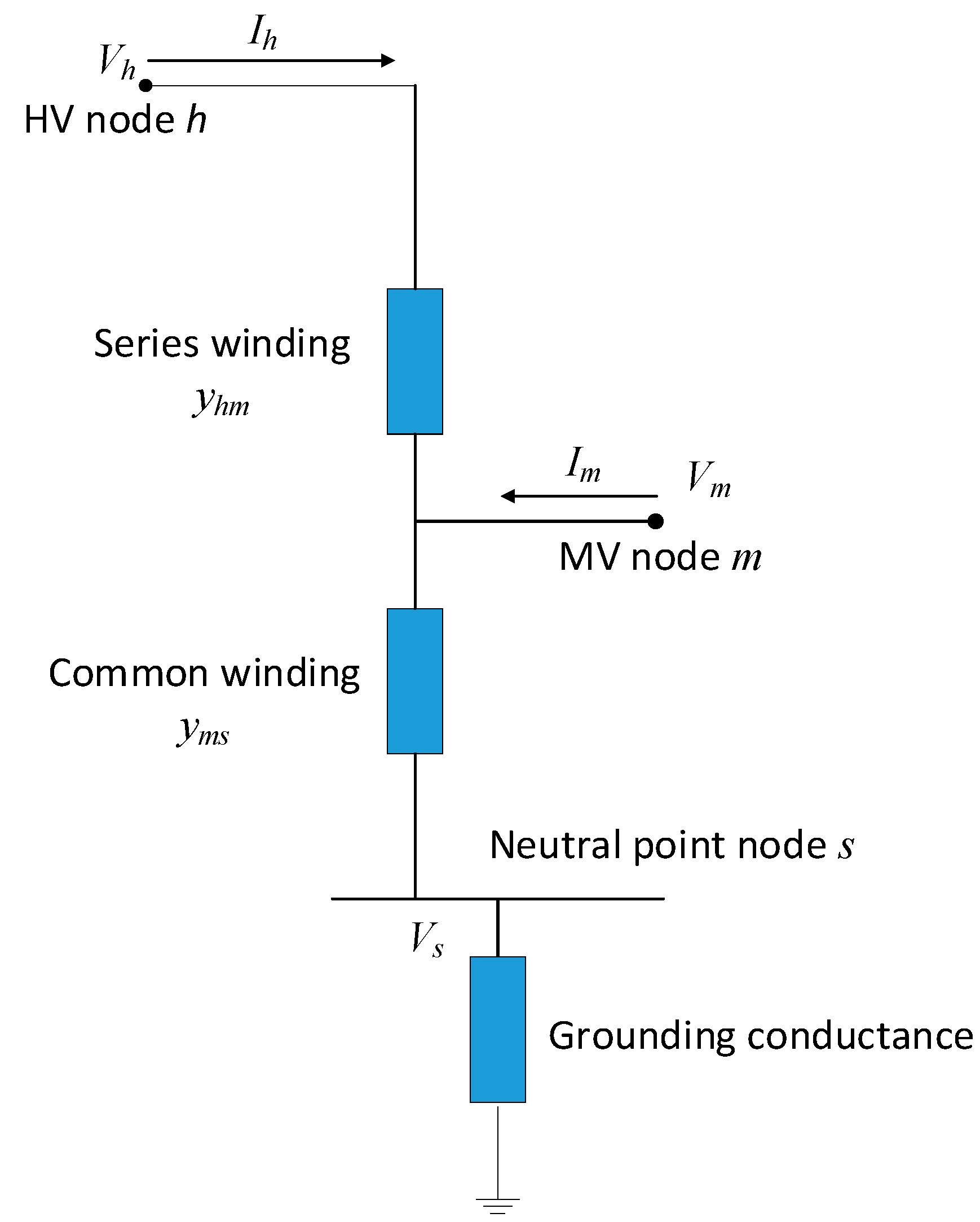
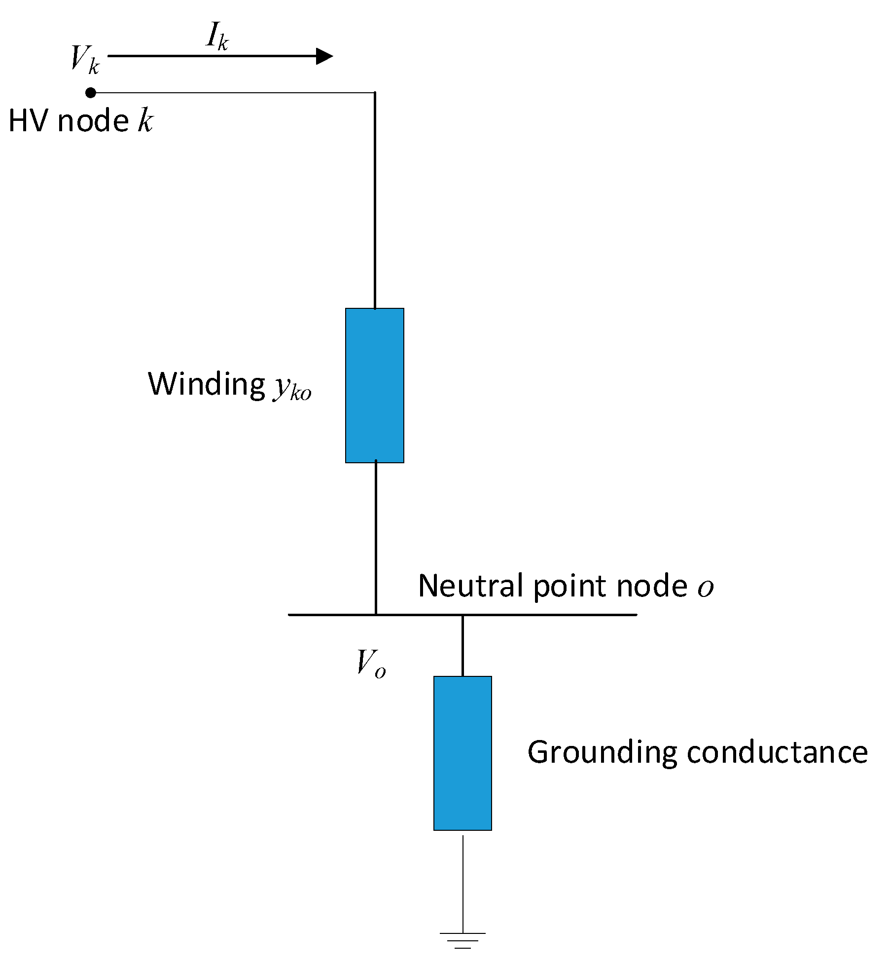
2.2. Bias Current Calculation Method
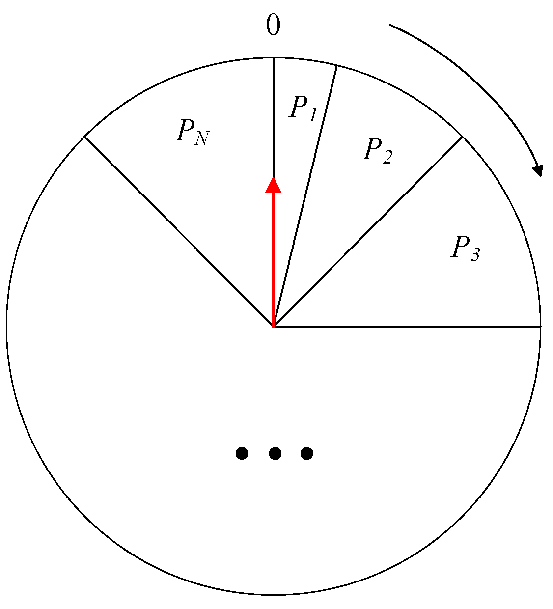
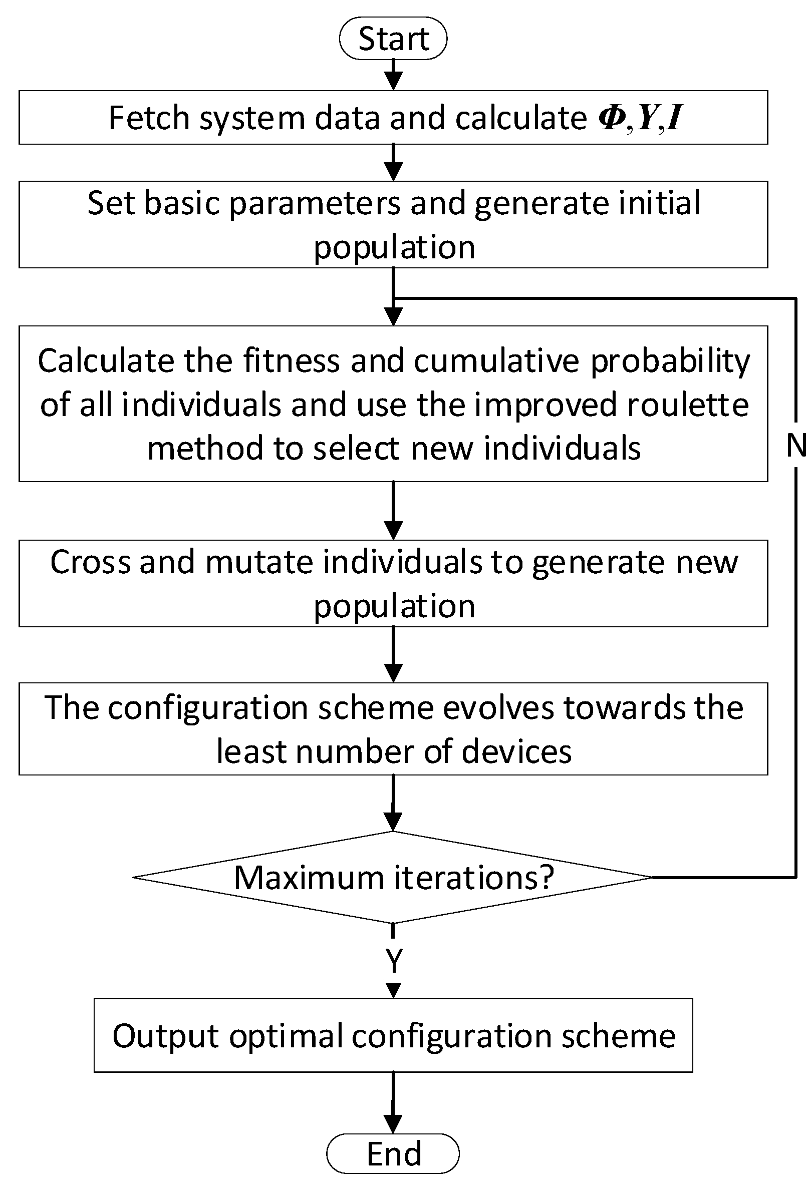
2.3. Combination Optimization Configuration Method for Capacitance and Resistance Devices
3. Results Analysis
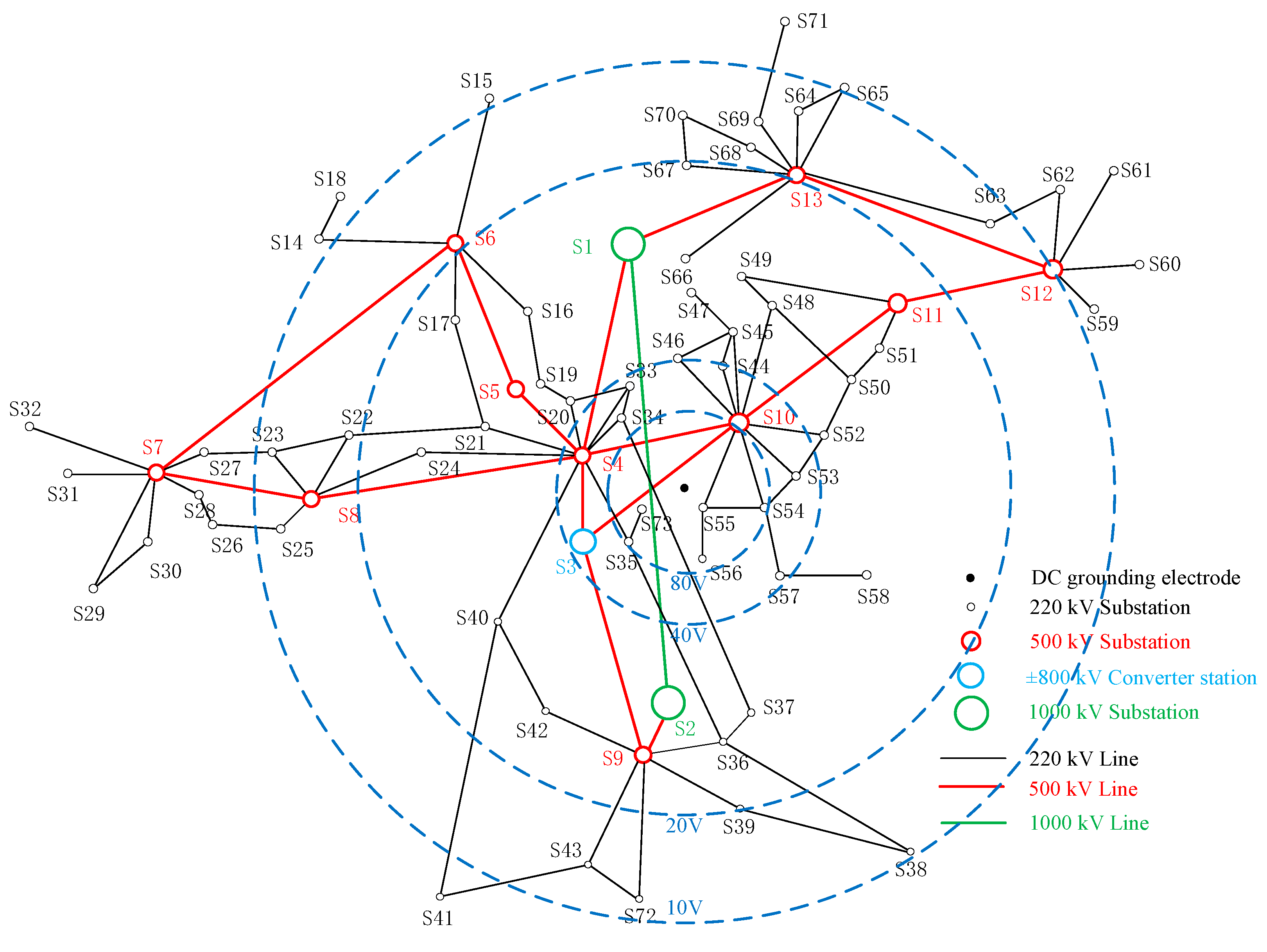
3.1. Test Network and Substation Ground Potential Calculation
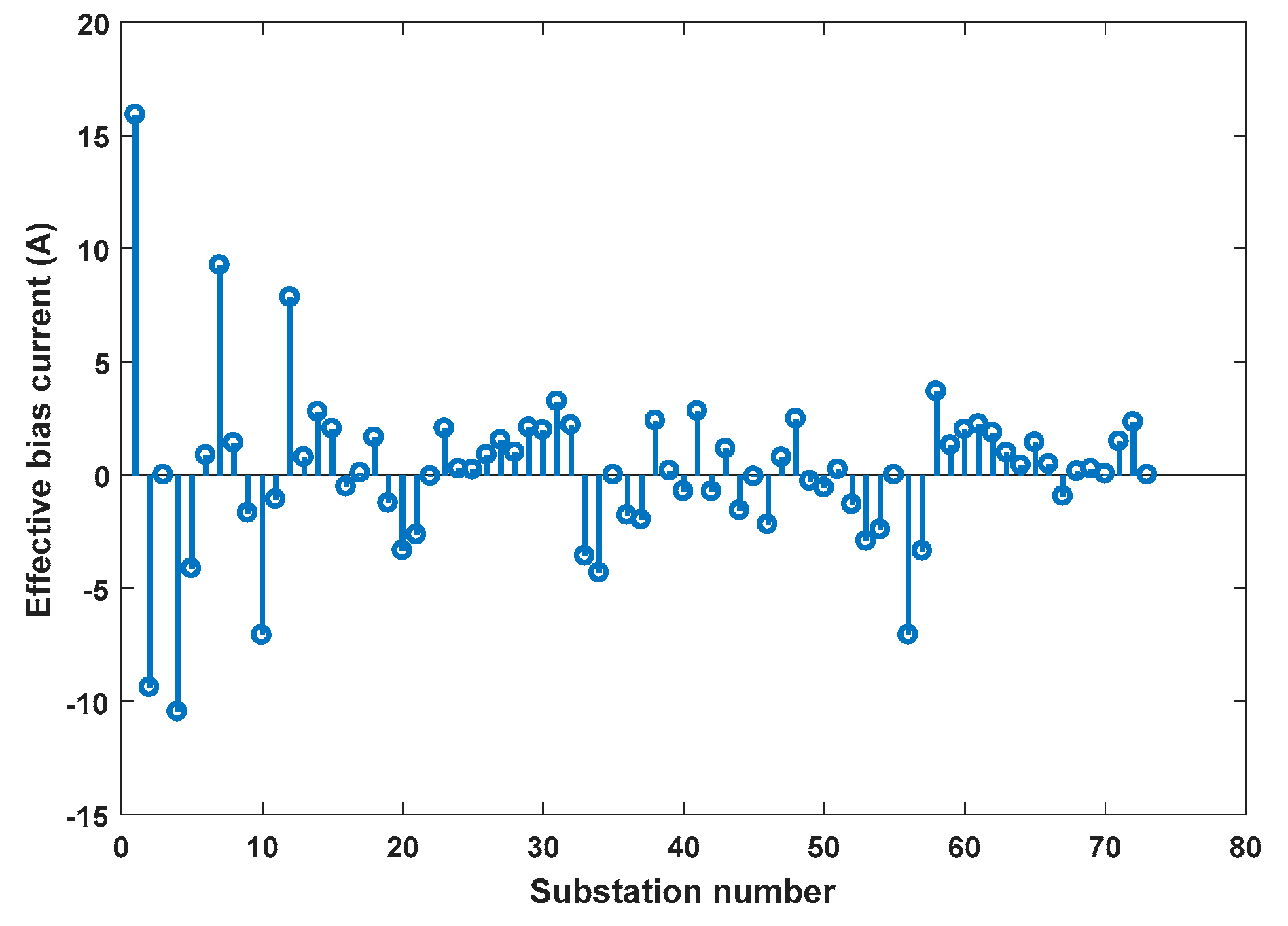
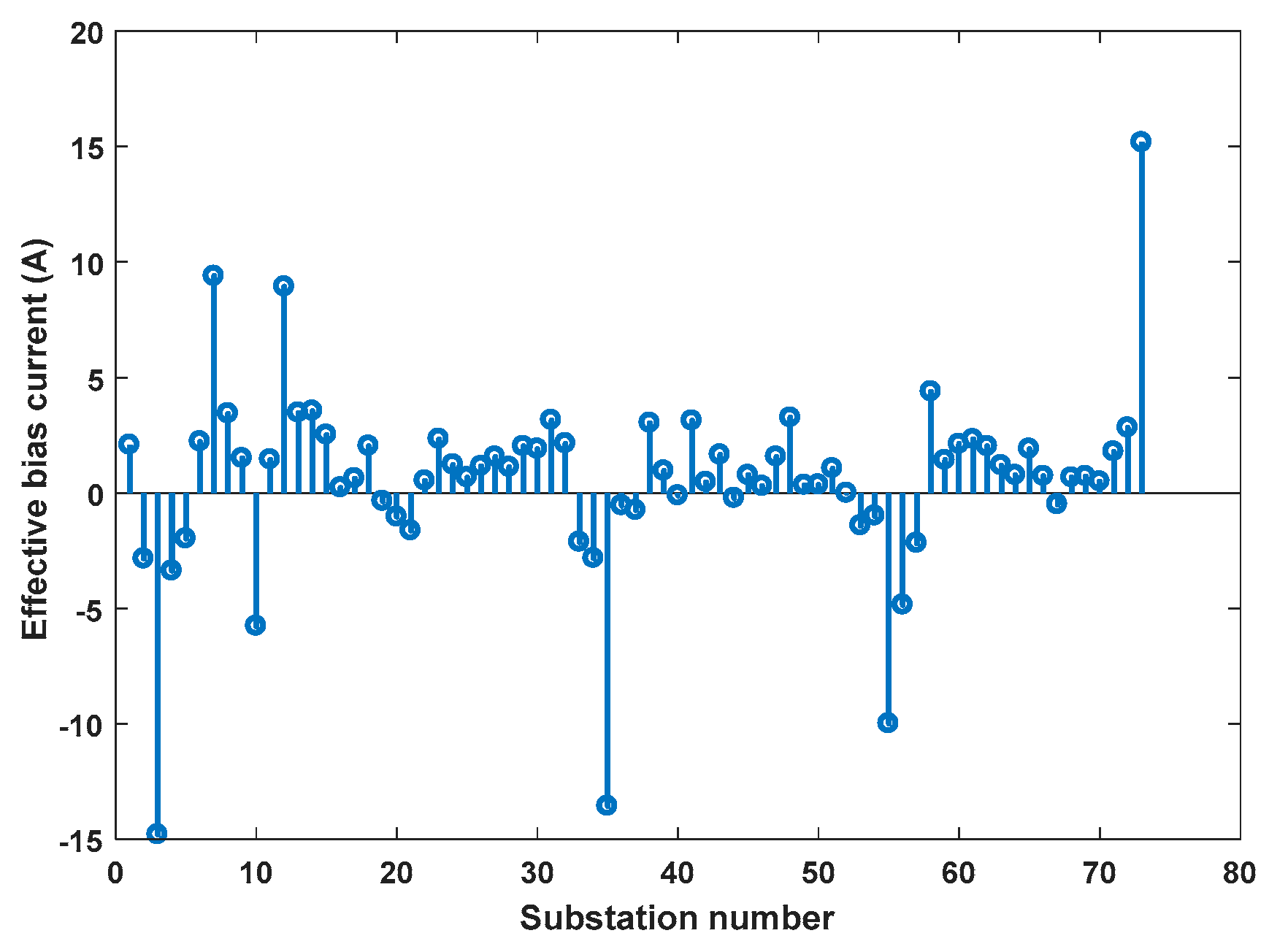
3.2. Effect of Devices on Effective Bias Current
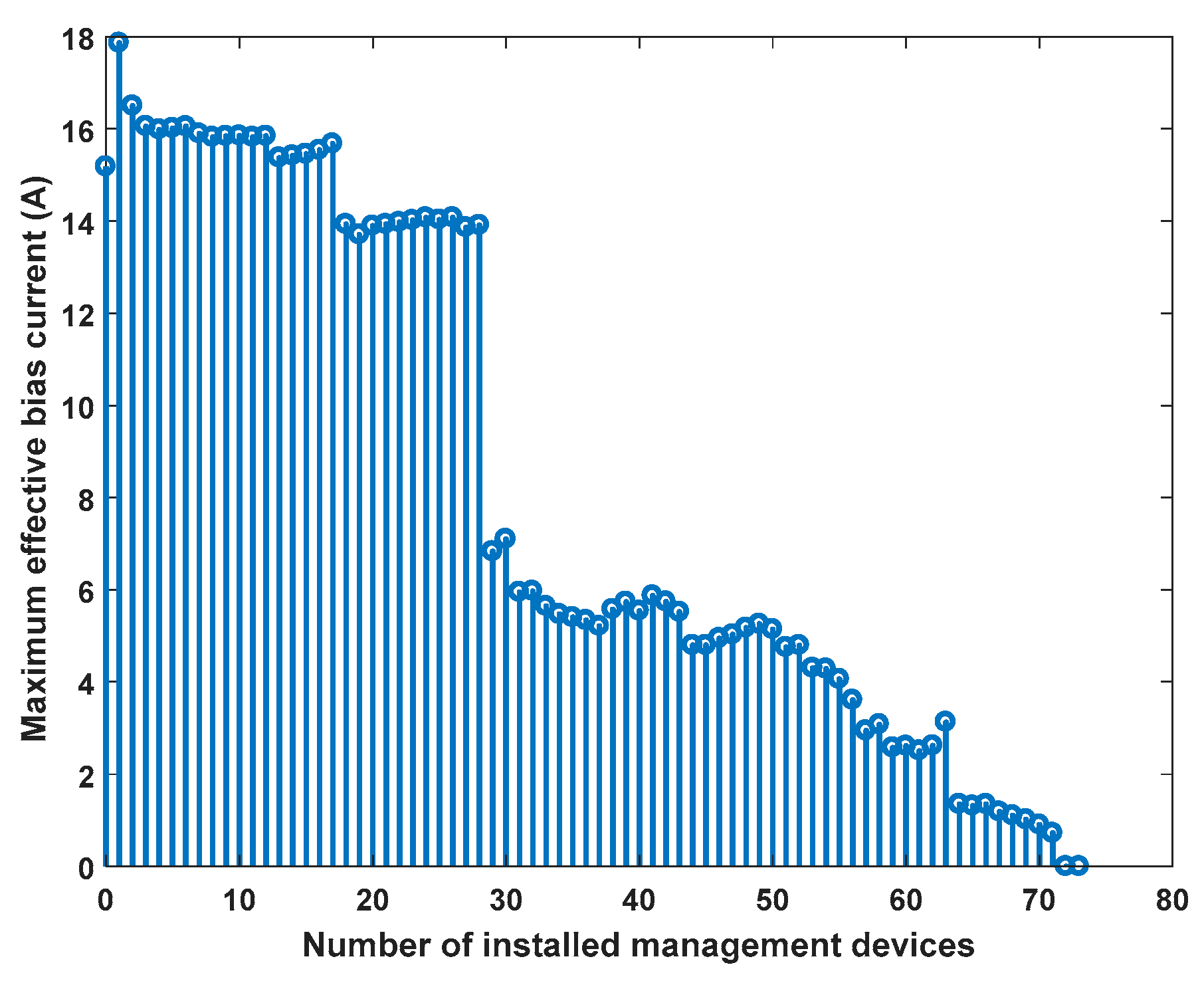
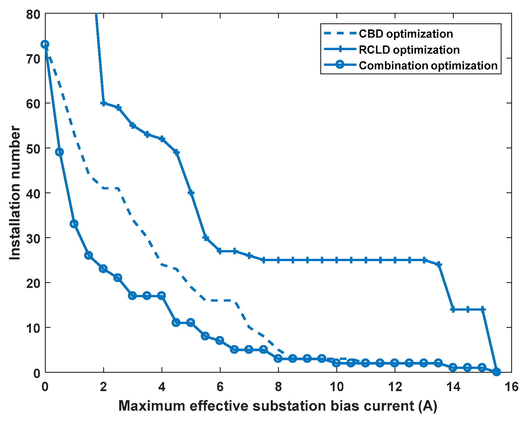
3.3. Optimization Strategy Results Analysis
4. Conclusions
Author Contributions
Funding
Conflicts of Interest
Nomenclature
| HVDC | high-voltage direct current |
| RCLD | resistance current limiting device |
| CBD | capacitance blocking device |
| HV | high voltage |
| MV | medium voltage |
| GIC | geomagnetically induced current |
References
- Liu, X.; Wu, J.; Lin, H.; Jadoon, A.; Wang, J. Research on DC bias analysis for transformer based on vibration Hilbert Huang transform and ground-state energy ratio method. Int. J. Elec. Power 2019, 109, 73–82. [Google Scholar] [CrossRef]
- Zhang, B.; Zhao, J.; Zeng, R.; He, J. Numerical analysis of DC current distribution in AC power system near HVDC system. IEEE Trans. Power Deliv. 2008, 23, 960–965. [Google Scholar] [CrossRef]
- Zhang, B.; Cui, X.; Zeng, R.; He, J. Calculation of DC current distribution in AC power system near HVDC system by using moment method coupled to circuit equations. IEEE Trans. Magn. 2006, 42, 703–706. [Google Scholar] [CrossRef]
- Mohammadi, F. Power Management Strategy in Multi-Terminal VSC-HVDC System. In Proceedings of the 4th National Conference on Applied Research in Electrical, Mechanical Computer and IT Engineering, Tehran, Iran, 4 October 2018. [Google Scholar]
- Liu, C.M.; Liu, L.G.; Pirjola, R. Geomagnetically induced currents in the high-voltage power grid in China. IEEE Trans. Power Deliv. 2009, 24, 2368–2374. [Google Scholar] [CrossRef]
- He, J.; Yu, Z.; Zeng, R.; Zhang, B. Vibration and audible noise characteristics of AC transformer caused by HVDC system under monopole operation. IEEE Trans. Power Deliv. 2012, 27, 1835–1842. [Google Scholar] [CrossRef]
- Moses, A. Measurement of magnetostriction and vibration with regard to transformer noise. IEEE Trans. Magn. 2003, 10, 154–156. [Google Scholar] [CrossRef]
- Adapa, R. High-wire act: HVDC technology: the state of the art. IEEE Power Energy Mag. 2012, 10, 18–29. [Google Scholar] [CrossRef]
- Li, W.; Pan, Z.; Lu, H.; Chen, X.; Zhang, L.; Wen, X. Influence of deep earth resistivity on HVDC ground-return currents distribution. IEEE Trans. Power Deliv. 2017, 32, 1844–1851. [Google Scholar] [CrossRef]
- Franck, C.M. HVDC circuit breakers: a review identifying future research needs. IEEE Trans. Power Deliv. 2011, 26, 998–1007. [Google Scholar] [CrossRef]
- Liu, X.; Yang, Y.; Huang, Y.; Jadoon, A. Vibration characteristic investigation on distribution transformer influenced by DC magnetic bias based on motion transmission model. Int. J. Elec. Power 2018, 98, 389–398. [Google Scholar] [CrossRef]
- Zhou, X.; Zhou, Z.; Ma, Y. Research on DC magnetic bias of power transformer. Procedia Eng. 2012, 29, 452–455. [Google Scholar] [CrossRef]
- Zhu, H.; Overbye, T.J. Blocking device placement for mitigating the effects of geomagnetically induced currents. IEEE Trans. Power Syst. 2015, 30, 2081–2089. [Google Scholar] [CrossRef]
- Li, X.; Wen, X.; Markham, P.N.; Liu, Y. Analysis of nonlinear characteristics for a three-phase, five-limb transformer under DC bias. IEEE Trans. Power Deliv. 2010, 25, 2504–2510. [Google Scholar] [CrossRef]
- Lu, H.; Zhang, J.; Yang, F.; Xu, B.; Liu, Z.; Zheng, Z.; Lan, L.; Wen, X. Improved secant method for getting proper initial magnetization in transformer DC bias simulation. Int. J. Elec. Power 2018, 103, 50–57. [Google Scholar] [CrossRef]
- Zhong, Z.; Zhang, S.; Zhao, J. Optimized configuration of DC bias current suppression resistors in HVDC based on MOFPSO. In Proceedings of the 2017 IEEE Applied Power Electronics Conference and Exposition (APEC), Tampa, FL, USA, 26–30 March 2017; pp. 1027–1032. [Google Scholar] [CrossRef]
- Dutta, S.; Bhattacharya, S. A method to measure the DC bias in high frequency isolation transformer of the dual active bridge DC to DC converter and its removal using current injection and PWM switching. In Proceedings of the 2014 IEEE Energy Conversion Congress and Exposition (ECCE), Pittsburgh, PA, USA, 14–18 September 2014; pp. 1134–1139. [Google Scholar] [CrossRef]
- Li, Y.; Li, Y.H.; Li, G.Q.; Zhao, D.B.; Chen, C. Two-stage multi-objective OPF for AC/DC grids with VSC-HVDC: Incorporating decisions analysis into optimization process. Energy 2018, 147, 286–296. [Google Scholar] [CrossRef]
- Pan, Z.H.; Wang, X.M.; Tan, B.; Zhu, L.; Liu, Y.; Liu, Y.L.; Wen, X.S. Potential compensation method for restraining the DC bias of transformers during HVDC monopolar operation. IEEE Trans. Power Deliv. 2016, 31, 103–111. [Google Scholar] [CrossRef]
- Xie, Z.; Lin, X.; Zhang, Z.; Li, Z.; Xiong, W.; Hu, H.; Khalid, M.S.; Adio, O.S. Advanced DC bias suppression strategy based on finite DC blocking devices. IEEE Trans. Power Deliv. 2017, 32, 2500–2509. [Google Scholar] [CrossRef]
- Pan, Z.; Zhang, L.; Wang, X.; Yao, H.; Zhu, L.; Liu, Y.; Wen, X. HVDC ground return current modeling in AC systems considering mutual resistances. IEEE Trans. Power Deliv. 2016, 31, 165–173. [Google Scholar] [CrossRef]
- Zou, D.; Li, S.; Kong, X.; Ouyang, H.; Li, Z. Solving the combined heat and power economic dispatch problems by an improved genetic algorithm and a new constraint handling strategy. Appl. Energy 2019, 237, 646–670. [Google Scholar] [CrossRef]
- Khalid, S. Performance evaluation of Adaptive Tabu search and Genetic Algorithm optimized shunt active power filter using neural network control for aircraft power utility of 400 Hz. J. Electr. Syst. Inf. Technol. 2018, 5, 723–734. [Google Scholar] [CrossRef]
- Hao, Y.; Wang, Q.; Li, Y.; Song, W. An intelligent algorithm for fault location on VSC-HVDC system. Int. J. Elec. Power 2018, 94, 116–123. [Google Scholar] [CrossRef]
- Anand, H.; Narang, N.; Dhillon, J.S. Multi-objective combined heat and power unit commitment using particle swarm optimization. Energy 2019, 172, 794–807. [Google Scholar] [CrossRef]
- Jamnani, J.G.; Pandya, M. Coordination of SVC and TCSC for management of power flow by particle swarm optimization. Energy Procedia 2019, 156, 321–326. [Google Scholar] [CrossRef]
- Zhang, W.; Maleki, A.; Rosen, M.A.; Liu, J. Optimization with a simulated annealing algorithm of a hybrid system for renewable energy including battery and hydrogen storage. Energy 2018, 163, 191–207. [Google Scholar] [CrossRef]
- Lenin, K.; Reddy, B.R.; Suryakalavathi, M. Hybrid Tabu search-simulated annealing method to solve optimal reactive power problem. Int. J. Elec. Power 2016, 82, 87–91. [Google Scholar] [CrossRef]


| Layer | Layer Depth/m | Resistivity/Ω·m |
|---|---|---|
| 1 | 0–45 | 50 |
| 2 | 45–155 | 250 |
| 3 | 155–300 | 2500 |
| 4 | 300–600 | 400 |
| 5 | 600–2000 | 1500 |
| 6 | >2000 | 4000 |
| Voltage Level/kV | Transformer Single-Phase Winding DC Resistance/Ω | Substation Grounding Resistance/Ω | Line Single-Phase Unit Length DC Resistance/Ω·km−1 | |
|---|---|---|---|---|
| HV Winding | MV Winding | |||
| 220 | 0.45 | - | 0.5 | 0.0748 |
| 500 | 0.238 | 0.097 | 0.2 | 0.0187 |
| 1000 | 0.183 | 0.141 | 0.1 | 0.0095 |
© 2019 by the authors. Licensee MDPI, Basel, Switzerland. This article is an open access article distributed under the terms and conditions of the Creative Commons Attribution (CC BY) license (http://creativecommons.org/licenses/by/4.0/).
Share and Cite
Wang, D.; Liu, C. Combination Optimization Configuration Method of Capacitance and Resistance Devices for Suppressing DC Bias in Transformers. Energies 2019, 12, 1813. https://doi.org/10.3390/en12091813
Wang D, Liu C. Combination Optimization Configuration Method of Capacitance and Resistance Devices for Suppressing DC Bias in Transformers. Energies. 2019; 12(9):1813. https://doi.org/10.3390/en12091813
Chicago/Turabian StyleWang, Donghui, and Chunming Liu. 2019. "Combination Optimization Configuration Method of Capacitance and Resistance Devices for Suppressing DC Bias in Transformers" Energies 12, no. 9: 1813. https://doi.org/10.3390/en12091813
APA StyleWang, D., & Liu, C. (2019). Combination Optimization Configuration Method of Capacitance and Resistance Devices for Suppressing DC Bias in Transformers. Energies, 12(9), 1813. https://doi.org/10.3390/en12091813