How Big Is an Error in the Analytical Calculation of Annular Fin Efficiency?

Abstract

An important role in the dimensioning of heat exchange surfaces with an annular fin is the fin efficiency. The fin efficiency is usually calculated using analytical expressions developed in the last century. However, these expressions are derived with certain assumptions and simplifications that involve a certain error in the calculation. The purpose of this paper is to determine the size of the error due to the assumptions and simplifications made when performing the analytical expression and to present what has the greatest impact on the amount of error, and give a recommendation on how to reduce that error. In order to determine the error, but also to gain a more detailed insight into the physics of heat exchange processes on the fin surface, computational fluid dynamics was applied to the original definition of fin efficiency. This means that a numerical simulation was performed for the actual fin material and for the ideal fin material with infinite thermal conductivity for the selected fin geometry and Re numbers from 2000 to 18,000. The results show that fin efficiency determined by numerical simulations is greater by up to 12.3% than the efficiency calculated analytically. The greatest impact on the amount of error is the assumption of the same temperature of the fin base surface and the outer tube surface and the assumption of equal heat transfer coefficient on the entire fin surface area. Using a newly recommended expression for the equivalent length of the fin tip, it would be possible to calculate the fin efficiency more precisely and thus the average heat transfer coefficient on the fin surface area, which leads to a more accurate dimensioning of the heat exchanger.

1. Introduction

Gas-liquid type heat exchangers are very widespread in industry. In order to increase the heat transfer, i.e., the reduction of the heat exchanger dimension, finned surfaces of different shapes have been developed. However, annular fins are most commonly used. Designing a heat exchanger with such finned surfaces is done on the basis of analytical solutions developed at the beginning of the 20th century. The first to analyse heat transfer on extended surfaces were Harper and Brown [1] in 1922. They introduced the concept of fin efficiency and provided analytical solutions for the two-dimensional model for a longitudinal and annular fin of uniform thickness. Also, they proposed the use of an adiabatic fin tip model with corrected fin height for the fin tip heat loss, which increases the fin height by half of the fin thickness.

In 1938, Murray [2] presented equations for the temperature gradient and fin effectiveness under conditions of a symmetrical temperature distribution around the radial fin base of uniform thickness. He also proposed a set of assumptions for extended surface analysis [2]. These limiting assumptions, which are referred to as the Murray–Gardner assumptions, are:

(a)

All temperatures and heat flow operate at steady-state levels.

(b)

The contact thermal resistance between the fin and the base surface is negligible.

(c)

There are no heat sources in the fin itself.

(d)

Radiation heat transfer from the fin is neglected.

(e)

The fin thickness is so small compared to its height that temperature gradients normal to the surface may be neglected.

(f)

The thermal conductivity of the fin and tube material is temperature-independent and uniform.

(g)

The temperature of the surrounding fluid is spatially uniform.

(h)

The heat-transfer coefficient is the same over all fin surfaces.

(i)

The temperature of the fin base surface is uniform and equal to the temperature of the tube base surface.

In 1945, Gardner [3] derived general equations for the temperature profile and fin efficiency for any form of extended surface for which the Murray–Gardner assumptions are applicable. Almost the same assumptions are applied by Darvishi at al. [4] in the numerical investigation for a hyperbolic annular fin with temperature-dependent thermal conductivity.

Ghai [5] investigated the validity of Gardner´s assumption of the constant heat transfer coefficient over the fin face. He has experimentally discovered large differences in the heat transfer coefficient from fin base to fin tip and along the fin surface in the air flow direction.

Based on the assumptions and the results of the research in the above-mentioned works, numerous analytical, experimental and numerical studies of heat transfer on finned surfaces have been performed for different geometries, materials and flow conditions. Heat transfer and the temperature distribution over the fin surface of the finned tube geometry with different fin perforation shape was investigated by Maki H. Zaidan et al. [6], applying a numerical analysis.

Nemati and Moghimi [7] studied the influence of different models of turbulence on the flow simulation that passes through a four-row tube heat exchanger. They found that K-Kl-ω, Transition SST and SST k-ω turbulence model show good match with experimental correlations.

Look and Krishnan [8] presented exact expressions for the correct terms for a one-dimensional fin temperature and heat loss when the insulated fin tip assumption is used for the case where the tip is maintained at a constant temperature.

Nemati and Samivand [9] have been numerically studying efficiency of the annular elliptical fin. They have proposed a simple correlation to approximate efficiency of the annular elliptical fin, applying the classic assumptions in determining the efficiency of annular fins.

Chen and Wang [10], in their trapezoid fin pattern research, apply standard expression for fin efficiency which does not take into account the temperature drop on the base surface of the fin.

H. J. Lane and P. J. Heggs [11] developed expressions for temperature profiles along the fins of different shapes: cone, trapezoid and dovetail fin, also with standard assumptions.

Cathal T. Ó Cléirigh, and William J. Smith [12] considered three shapes of spiral fins: full, partially segmented and fully segmented. The stationary state model with two equations of the turbulent model was chosen and the flow in Reynolds numbers 5000 to 30,000, respectively. The Nusselt number and the pressure drop calculated with the CFD software were compared with the correlations in the experimental literature.

The question is: what is the size of error in the calculation of the fin efficiency due to the above assumptions and simplifications applied to the physical model of heat exchange with fin surfaces? And, can this error be reduced? In this regard, the subjects of interest in this paper are the assumptions mentioned under (h) and (i) and their impact on the accuracy of the calculation of the fin efficiency.

It is clear that if fins increase the heat transfer, then heat must be transferred by conduction to the fin base surface from remote regions of the tube, and this conductive transport needs a temperature drop. Conduction through the fin cross section and convective heat transfer over the fin surface area are carried out at the same time. This is possible only if there is a temperature difference between the fin base surface and the fin tip as a driving force. Because of this, the fins have an average temperature lower than that of the unfinned part of the tube. Therefore, the efficiency of the fins is different to that of the unfinned part of the tube because the heat transfer between fin surface area and surrounding fluid takes place with a smaller temperature difference than between the unfinned part of the tube surface area and the fluid.

The assumption is that the magnitude of the error can be determined by applying numerical analysis to the original definition of the fin efficiency, which also provides a more detailed insight into the physics of the heat exchange process on finned surfaces.

The idea is to obtain quantitative data on temperature and heat exchanged on the particular surfaces of the annular fin of the constant thickness for the “ideal fin” and the real fin by numerical analysis. After that, the fin efficiency is calculated by using numerical simulation data, conventional analytical equations and Murray–Gardner assumptions. By comparing the results, it is possible to calculate the magnitude of the error resulting from the application of common expressions and assumptions. To the authors’ knowledge, fin efficiency analysis has not been performed in this way so far.

2. Materials and Methods

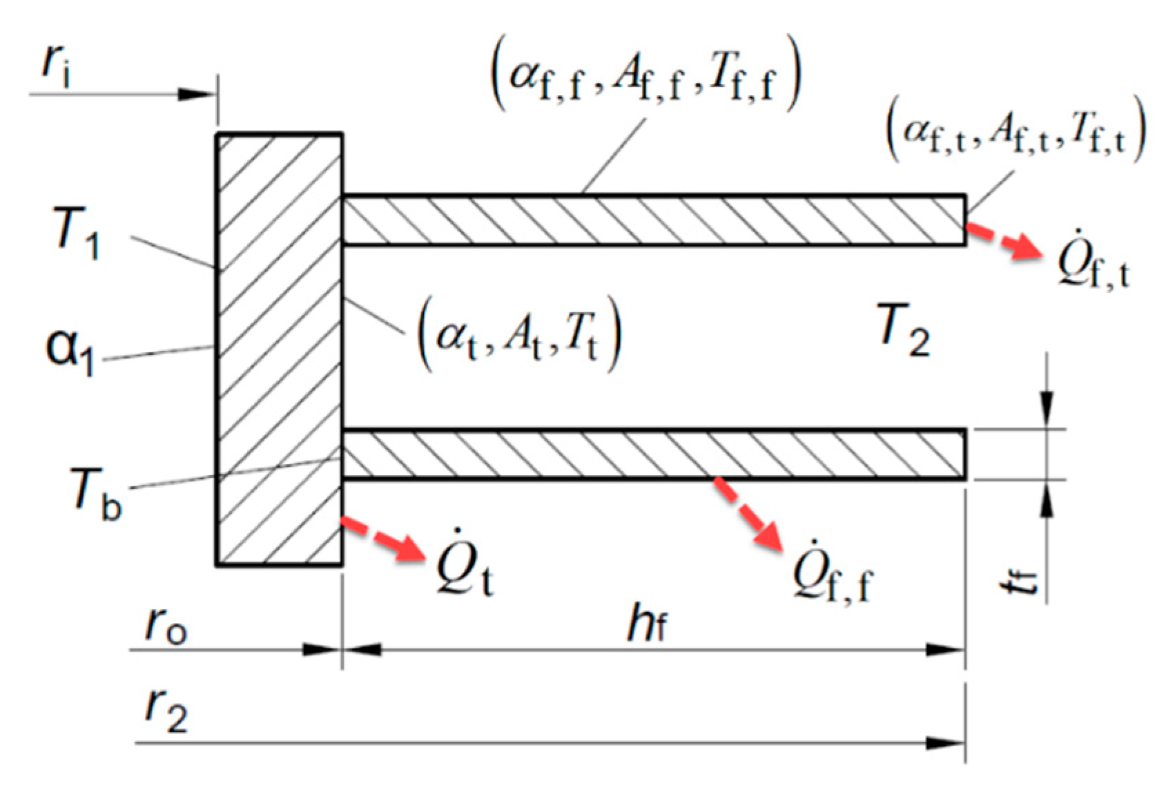
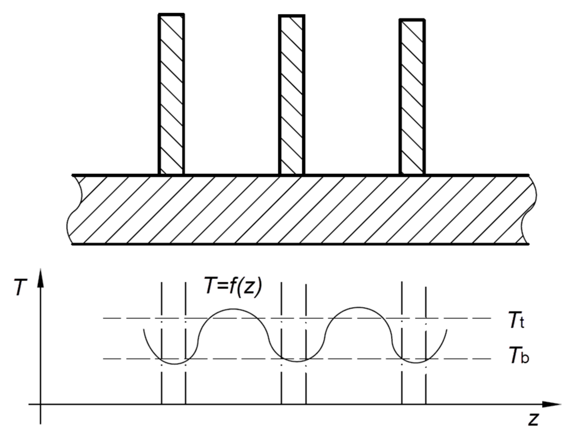
2.1. Physical Basis of Heat Exchange on Finned Surfaces

In order to present the impact of the Murray–Gardner assumptions and simplifications, the physical model of heat exchange on the annular fin is presented and analysed in detail. Over the fin surface and the outer tube wall surface, heat is transferred by convection to the surrounding fluid. Specific consideration is given to the case with the same fin and tube material, i.e., same thermal conductivity. In theoretical consideration, the average temperature of the tube base area is T_t and the average temperature of the fin base area is T_b. The total heat transfer rate is equal to the sum of the heat transfer rate through the surface area of the fins ${\dot{Q}}_{\mathrm{f}}$ and through the unfinned surface area of the tube ${\dot{Q}}_{\mathrm{t}}$:

$$\dot{Q}={\dot{Q}}_{\mathrm{t}}+{\dot{Q}}_{\mathrm{f}}.$$

(1)

Heat transfer rate through the fin surface consists of heat transfer rate through the fin face surfaces ${\dot{Q}}_{\mathrm{f},\mathrm{f}}$ and through the fin tip surface ${\dot{Q}}_{\mathrm{f}.\mathrm{t}}$ as shown in Figure 1. The temperature in the fin falls from T_b at the fin base surface to T_f,t at its tip.

The heat transfer rate ${\dot{Q}}_{\mathrm{t}}$ from the finless tube surface A_t in the fluid is defined with Equation (2).

$${\dot{Q}}_{\mathrm{t}}={\alpha }_{\mathrm{t}}{A}_{\mathrm{t}}\left(T_{\mathrm{t}}-T_2\right),$$

(2)

where α_t is the associated average heat transfer coefficient. The heat transfer rate ${\dot{Q}}_{\mathrm{f}}$ from fin surfaces A_f to the fluid is defined with Equations (3) to (5) (Figure 1).

$${\dot{Q}}_{\mathrm{f}}={\dot{Q}}_{\mathrm{f},\mathrm{f}}+{\dot{Q}}_{\mathrm{f},\mathrm{t}},$$

(3)

$${\dot{Q}}_{\mathrm{f},\mathrm{f}}={\alpha }_{\mathrm{f},\mathrm{f}}{A}_{\mathrm{f},\mathrm{f}}\left(T_{\mathrm{f},\mathrm{f}}-T_2\right),$$

(4)

$${\dot{Q}}_{\mathrm{f},\mathrm{t}}={\alpha }_{\mathrm{f},\mathrm{t}}{A}_{\mathrm{f},\mathrm{t}}\left(T_{\mathrm{f},\mathrm{t}}-T_2\right).$$

(5)

The total heat transfer rate from fin surfaces to the fluid is defined with Equation (6).

$${\dot{Q}}_{\mathrm{f}}={\alpha }_{\mathrm{f},\mathrm{f}}{A}_{\mathrm{f},\mathrm{f}}\left(T_{\mathrm{f},\mathrm{f}}-T_2\right)+{\alpha }_{\mathrm{f},\mathrm{t}}{A}_{\mathrm{f},\mathrm{t}}\left(T_{\mathrm{f},\mathrm{t}}-T_2\right).$$

(6)

The total fin surface area is the sum of the fin face surface area and the fin tip surface area:

$$A_{\mathrm{f}}=A_{\mathrm{f},\mathrm{f}}+A_{\mathrm{f},\mathrm{t}}.$$

(7)

The average heat transfer coefficient for all fin surfaces can be defined as:

$${\alpha }_{\mathrm{f}}=\frac{{\alpha }_{\mathrm{f},\mathrm{f}}\cdot A_{\mathrm{f},\mathrm{f}}+{\alpha }_{\mathrm{f},\mathrm{t}}\cdot A_{\mathrm{f},\mathrm{t}}}{A_{\mathrm{f},\mathrm{f}}+A_{\mathrm{f},\mathrm{t}}}.$$

(8)

The average temperature for all fin surfaces can be defined as:

$$T_{\mathrm{f}}=\frac{T_{\mathrm{f},\mathrm{f}}\cdot A_{\mathrm{f},\mathrm{f}}+T_{\mathrm{f},\mathrm{t}}\cdot A_{\mathrm{f},\mathrm{t}}}{A_{\mathrm{f},\mathrm{f}}+A_{\mathrm{f},\mathrm{t}}}.$$

(9)

The heat transfer rate from fin to the fluid applying Equations (8) and (9) will be:

$${\dot{Q}}_{\mathrm{f}}={\alpha }_{\mathrm{f}}{A}_{\mathrm{f}}\left(T_{\mathrm{f}}-T_2\right).$$

(10)

The fin’s thermal performance is expressed by the fin efficiency. The maximum driving potential for convection is the difference between the fin base temperature T_b and the bulk fluid temperature T₂. Hence, the fin efficiency is defined as the ratio of the actual fin heat flux to its heat flux if the entire surface of ideal nonexisting fin were at the same temperature as its base surface area, where the fin material has an infinite thermal conductivity. However, since any fin has a finite conductivity resistance, a temperature gradient must exist along the fin. Definition of the fin efficiency therefore can be expressed as:

$${\eta }_{\mathrm{f}}=\frac{{\dot{Q}}_{\mathrm{f}}}{{\dot{Q}}_{\mathrm{f},\max }}.$$

(11)

The fin efficiency is an idealisation and has physically no meaning. An ideal fin has infinite thermal conductivity λ_f of the fin material and the same geometry and operating conditions as the actual fin. Under these assumptions, the ideal fin is at the uniform base surface temperature T_b so T_b ≈ T_t = T_f,f = T_f,t and the heat transfer coefficient α_t,λ=∞ ≈ α_t, α_f,λ=∞ ≈ α_f, α_f,f,λ=∞ ≈ α_f,f, α_f,t,λ=∞ ≈ α_f,t. We could write:

$${\dot{Q}}_{\mathrm{f},\max }={\alpha }_{\mathrm{f},\mathrm{f}}{A}_{\mathrm{f},\mathrm{f}}\left(T_{\mathrm{t}}-T_2\right)+{\alpha }_{\mathrm{f},\mathrm{t}}{A}_{\mathrm{f},\mathrm{t}}\left(T_{\mathrm{t}}-T_2\right)=\left({\alpha }_{\mathrm{f},\mathrm{f}}{A}_{\mathrm{f},\mathrm{f}}+{\alpha }_{\mathrm{f},\mathrm{t}}{A}_{\mathrm{f},\mathrm{t}}\right)\left(T_{\mathrm{t}}-T_2\right).$$

(12)

Applying Equation(8) in Equation(12) follows that:

$${\dot{Q}}_{\mathrm{f},\max }={\alpha }_{\mathrm{f}}{A}_{\mathrm{f}}(T_{\mathrm{t}}-T_2),$$

(13)

$${\eta }_{\mathrm{f}}=\frac{{\dot{Q}}_{\mathrm{f}}}{{\dot{Q}}_{\mathrm{f},\max }}=\frac{{\alpha }_{\mathrm{f}}{A}_{\mathrm{f}}\left(T_{\mathrm{f}}-T_2\right)}{{\alpha }_{\mathrm{f}}{A}_{\mathrm{f}}(T_{\mathrm{t}}-T_2)}=\frac{T_{\mathrm{f}}-T_2}{T_{\mathrm{t}}-T_2}.$$

(14)

Equation (14) shows that ${\eta }_{\mathrm{f}}$ actually corrects the mean temperature difference between the fin surface and the surrounding fluid, which is necessary because the temperature along the fin surface is not constant. From Equation (14), it follows that:

$${\dot{Q}}_{\mathrm{f}}={\eta }_{\mathrm{f}}{\alpha }_{\mathrm{f}}{A}_{\mathrm{f}}(T_{\mathrm{t}}-T_2).$$

(15)

Fin efficiency is always less than one. It depends on both the heat conduction processes in the fin and the convective heat transfer, which influence each other.

In reality, the average temperature of the fin base surface T_b is different from the unfinned tube wall temperature T_t. The heat transfer rate through the fin base surface into the fin is significantly higher than the heat transfer rate from the unfinned part of the tube wall into the fluid. The temperature drop, which appears underneath the fin, causes a periodic temperature profile to develop in the tube wall. This is shown schematically in Figure 2. The temperature drop is higher as the temperature conductivity of the material is lower.

In the literature [13,14], it is often assumed that:

$$T_{\mathrm{b}}=T_{\mathrm{t}}.$$

(16)

This simplification leads to an overestimation of the heat transfer rate. The calculated heat transfer rate can be as much as 25% bigger than it actually is, as shown by Sparrow and Hennecke [15] as well as Sparrow and L. Lee [16]. Using Equations (15) and (16) leads to:

$$\dot{Q}={\dot{Q}}_{\mathrm{t}}+{\dot{Q}}_{\mathrm{f}}={\alpha }_{\mathrm{t}}{A}_{\mathrm{t}}(T_{\mathrm{t}}-T_2)+{\eta }_{\mathrm{f}}{\alpha }_{\mathrm{f}}{A}_{\mathrm{f}}(T_{\mathrm{t}}-T_2).$$

(17)

For thin fins densely spaced A_f >> A_t, so in the Equation (17) the second term is more important, although η_f < 1. Therefore, as ${\alpha }_{\mathrm{t}}\approx {\alpha }_{\mathrm{f}}$ in set in the literature, we could write:

$$\dot{Q}={\alpha }_{\mathrm{f}}\left(A_{\mathrm{t}}+{\eta }_{\mathrm{f}}{A}_{\mathrm{f}}\right)(T_{\mathrm{t}}-T_2).$$

(18)

The overall surface efficiency that includes fins and unfinned part of the tube is defined with Equation (19).

$${\eta }_{\mathrm{o}}=\frac{\dot{Q}}{{\dot{Q}}_{\max }}.$$

(19)

${\dot{Q}}_{\max }$ is the maximum heat transfer rate for ideal fin, which is obtained by setting ${\eta }_{\mathrm{f}}=1$ in Equation (18):

$${\dot{Q}}_{\max }={\alpha }_{\mathrm{f}}\left(A_{\mathrm{t}}+A_{\mathrm{f}}\right)(T_{\mathrm{t}}-T_2).$$

(20)

With this we could write:

$${\eta }_{\mathrm{o}}=\frac{\dot{Q}}{{\alpha }_{\mathrm{f}}\left(A_{\mathrm{t}}+A_{\mathrm{f}}\right)(T_{\mathrm{t}}-T_2)}.$$

(21)

Substituting Equations (18) and (20) into Equation(21) yields:

$${\eta }_{\mathrm{o}}=1-\frac{A_{\mathrm{f}}}{A_{\mathrm{t}}+A_{\mathrm{f}}}(1-{\eta }_{\mathrm{f}}).$$

(22)

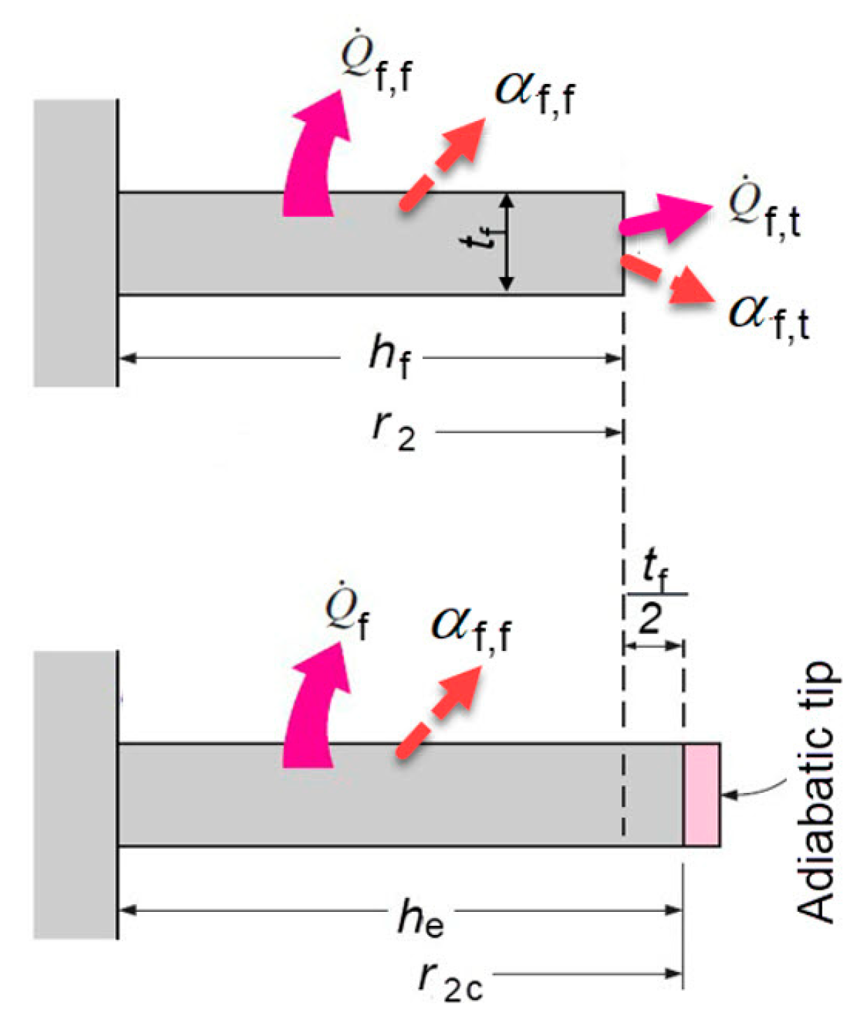
2.2. Analytical Solution of Fin Efficiency

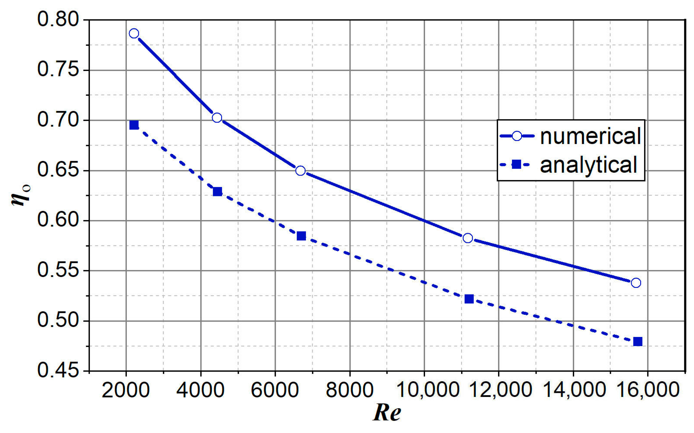
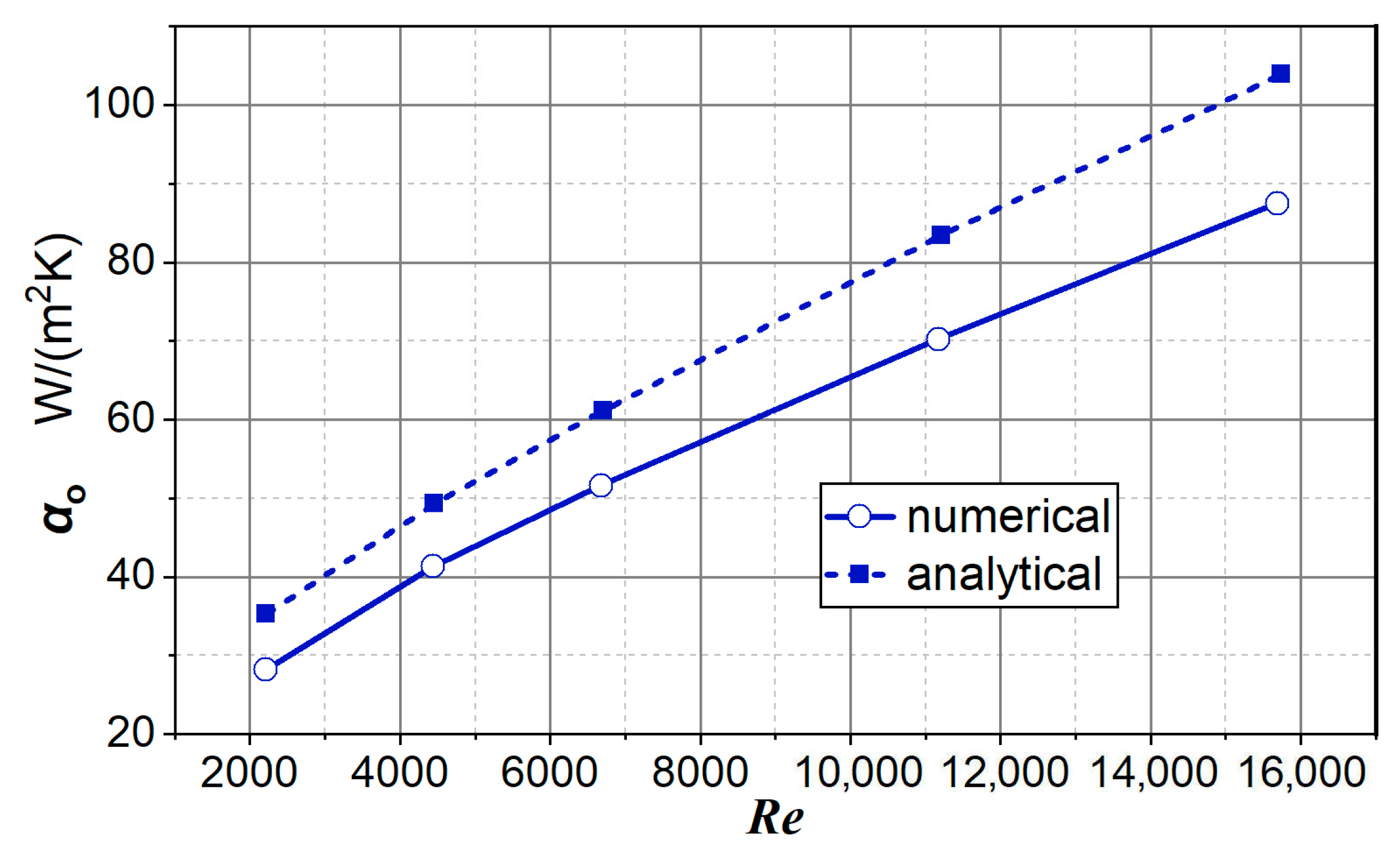
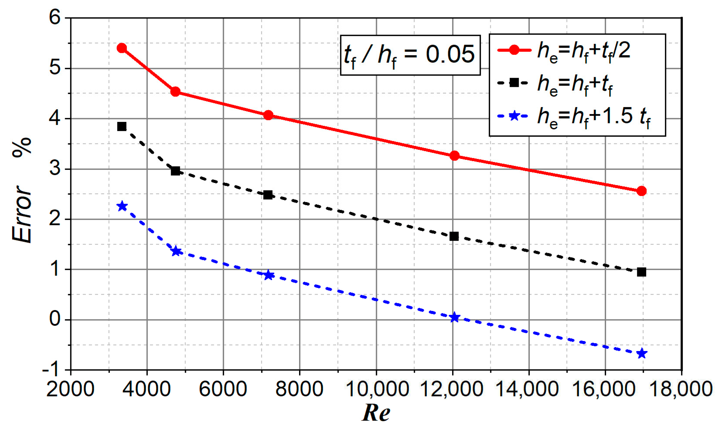
In general, theoretical fin efficiency is defined as follows:

$${\eta }_{\mathrm{f}}=\frac{\mathrm{The}\mathrm{actual}\mathrm{heat}\mathrm{transfer}\mathrm{rate}}{\begin{array}{c}\mathrm{Maximum}\mathrm{heat}\mathrm{transfer}\mathrm{rate}\mathrm{when}\mathrm{the}\mathrm{entire}\mathrm{fin}\\ \mathrm{was}\mathrm{at}\mathrm{the}\mathrm{base}\mathrm{surface}\mathrm{temperature}\end{array}}.$$

(23)

The theoretical efficiency of an annular fin is calculated according to [13,14]:

$${\eta }_{\mathrm{f},\mathrm{th}}=C_2\frac{K_1(m\cdot r_{\mathrm{o}})\cdot I_1(m\cdot r_{2c})-I_1(m\cdot r_{\mathrm{o}})\cdot K_1(m\cdot r_{2c})}{I_0(m\cdot r_{\mathrm{o}})\cdot K_1(m\cdot r_{2c})+K_0(m\cdot r_{\mathrm{o}})\cdot I_1(m\cdot r_{2c})}.$$

(24)

K₀, I₀ are modified Bessel’s functions of the zero order, first and second types, a K₁, I₁ are the modified Bessel’ function of the first order, first and the second type. With the aim of simplifying calculations, the analytical expression for the corrected fin radius, r_2c is introduced (Figure 3). It is based on the assumption of equivalence between the heat transferred from the actual fin with tip convection and the heat transferred from a longer, hypothetical fin with an adiabatic tip [1,13]. The corrected fin radius is defined with:

$$r_{2\mathrm{c}}=r_2+\frac{t_{\mathrm{f}}}{2}.$$

(25)

This assumption increases fin surface area in the corresponding amount but does not include a greater heat transfer coefficient at the fin tip in regards to the heat transfer coefficient at the fin face surface. This enters also a certain error in the fin efficiency calculation.

Table 1. The share of individual surfaces in the total surface area.

Surface	Area (mm2)	Share (%)
Unfinned tube surface	628.32	11.4
Fin face surface	4712.39	85.7
Fin tip surface	157.08	2.9
Total surface area	5497.78	100.0

shows the proportion of individual surfaces in the total tube finned surface area.

Parameters m and C₂ are defined with:

$$m=\sqrt{\frac{2{\alpha }_0}{{\lambda }_{\mathrm{f}}\cdot t_{\mathrm{f}}}},$$

(26)

$$C_2=\frac{2\cdot r_{\mathrm{o}}}{m\cdot (r_{2\mathrm{c}}^2-r_{\mathrm{o}}^2)}.$$

(27)

Comparing experimentally obtained fin efficiencies with the analytical solutions, an empirical correction factor was obtained. For annular fin this correction factor has the form [17]:

$$E=0.76+0.24\cdot {\eta }_{\mathrm{f},\mathrm{th}},$$

(28)

$${\eta }_{\mathrm{f}}=E\cdot {\eta }_{\mathrm{f},\mathrm{th}}.$$

(29)

The actual average gas-side convective heat transfer coefficient α₀ is calculated applying fin efficiency:

$${\alpha }_0=\frac{{\alpha }_e\cdot (A_{\mathrm{t}}+A_{\mathrm{f}})}{(A_{\mathrm{t}}+{\eta }_{\mathrm{f}}\cdot A_{\mathrm{f}})}.$$

(30)

The effective/apparent airside convective heat transfer coefficient α_e is:

$${\alpha }_{\mathrm{e}}=\frac{1}{\left(\frac{1}{U}-(A_t+A_{\mathrm{f}})\frac{\ln \frac{r_{\mathrm{o}}}{r_{\mathrm{i}}}}{2\pi L{N}_{\mathrm{t}}{\lambda }_{\mathrm{t}}}-\frac{(A_{\mathrm{t}}+A_{\mathrm{f}})}{A_{\mathrm{t},\mathrm{i}}{\alpha }_{\mathrm{i}}}\right)}.$$

(31)

L is the tube length, N_t is the total number of tubes, A_t,i is the tube side surface area and α_i is the tube side convective heat transfer coefficient. The overall heat transfer coefficient U referenced to (or based on) the outside tube heat transfer area is calculated according to Equation (32):

$$U=\frac{\dot{Q}}{(A_{\mathrm{t}}+A_{\mathrm{f}})\cdot \Delta T_{\ln }}.$$

(32)

It is important to note that the mean logarithmic temperature difference (ΔT_ln) in the concept of fin efficiency is calculated by applying the (maximum) temperature of the outer surface of the tube. In our case, the logarithmic mean temperature difference for counter-current flow acc. to Equation (33) is used:

$$\mathsf{\Delta }{\mathrm{T}}_{\ln }=\frac{T_{\mathrm{in}}-T_{\mathrm{out}}}{\ln \frac{T_{\mathrm{in}}-T_{\mathrm{t}}}{T_{\mathrm{out}}-T_{\mathrm{t}}}}$$

(33)

T_in and T_out is the air temperature at the inlet and outlet of the heat exchanger.

3. Results

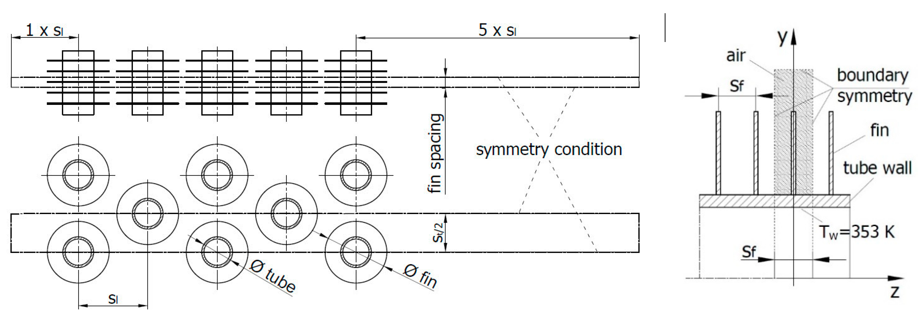
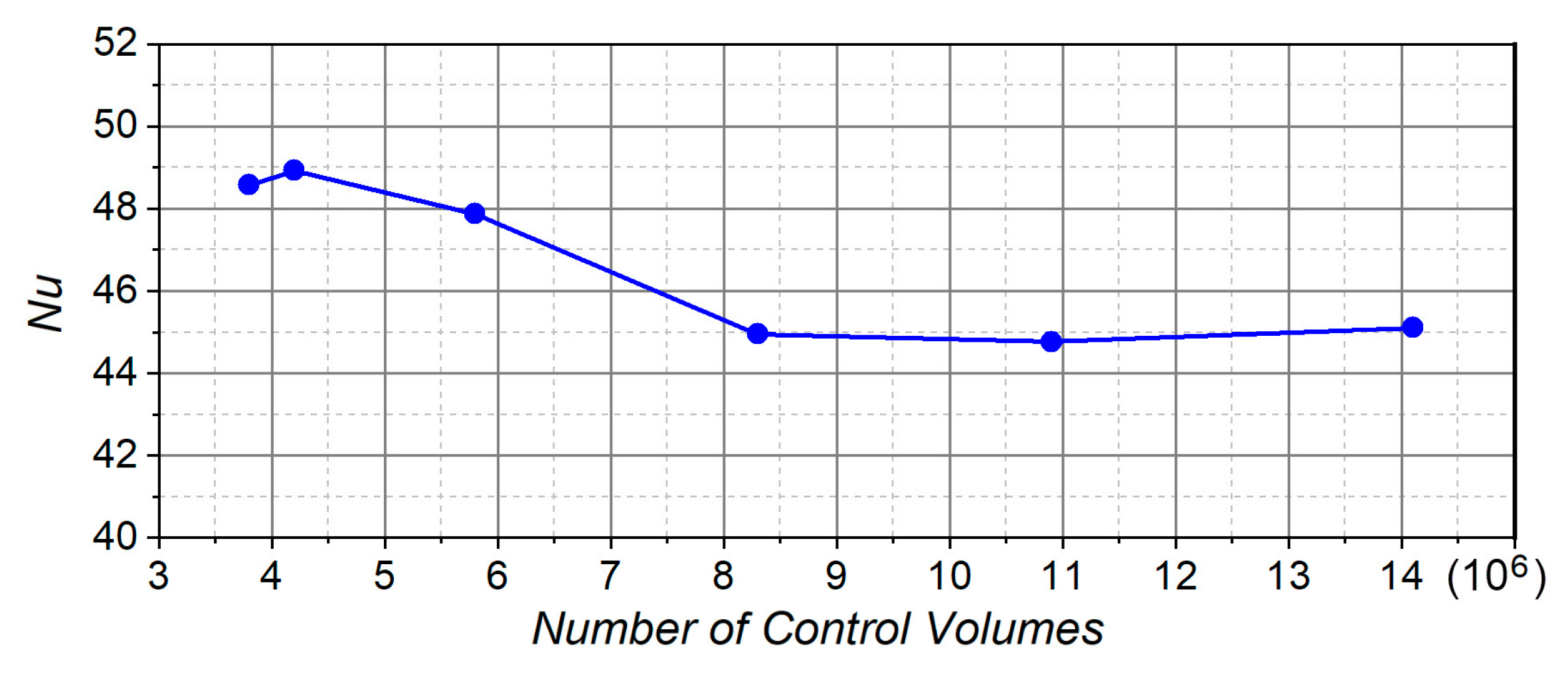
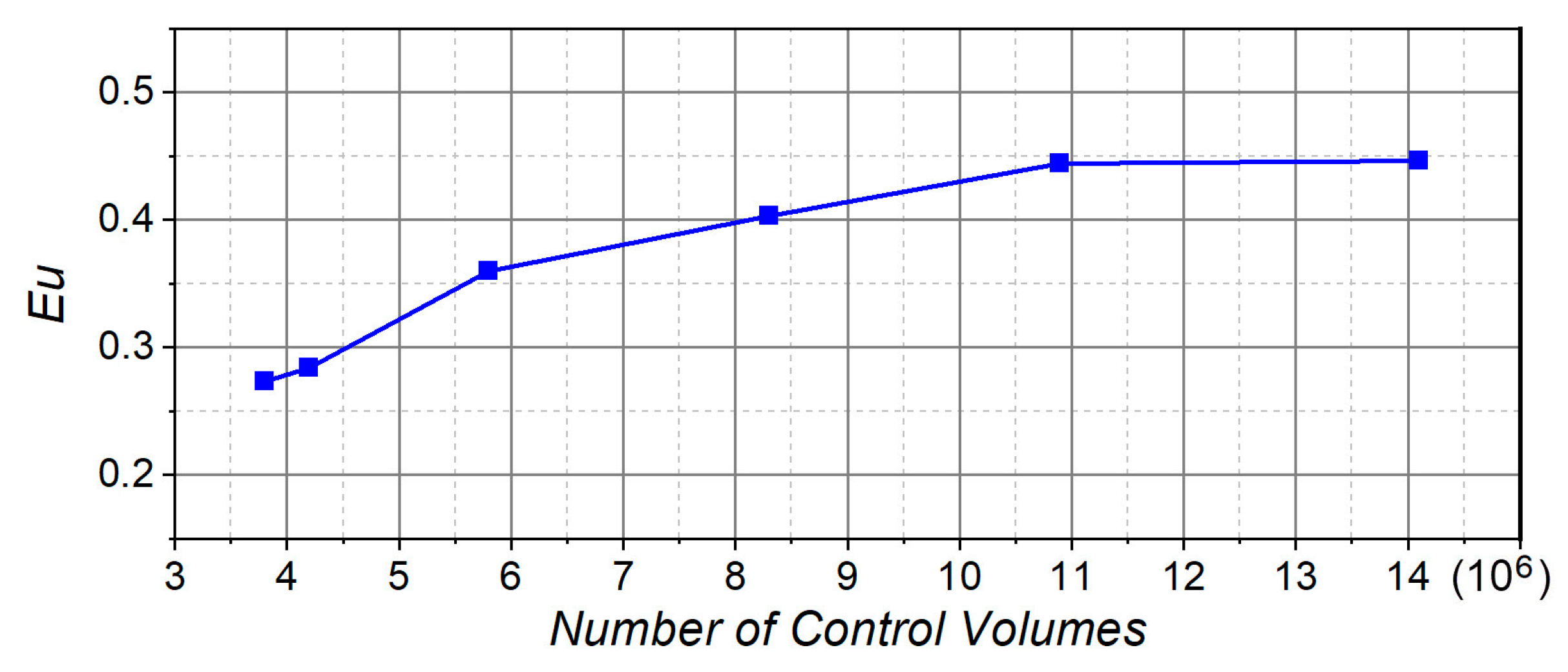
3.1. Numerical Analysis

In this paper, for research implementation, the tube Ø20×1.5 is selected. As a reference geometry, an annular fin Ø40/Ø20 with a thickness of 0.5 mm was selected. The fin is used as a cooling fin. The fin and tube material is stainless steel. Characteristic dimensions of the tube and fins are presented in

Table 2. Characteristic dimensions of tube and fins.

Tube Outside Diameter	do	mm	20
Tube inside diameter	di	mm	17
Tube rows configuration	-	-	staggered
Transverse tube pitch	st	mm	50
Longitudinal tube pitch	sl	mm	40
Fin height	hf	mm	10
Fin thickness	tf	mm	0.5
Fin pitch	sf	mm	4.5
Number of tube rows	Nl	-	5

.

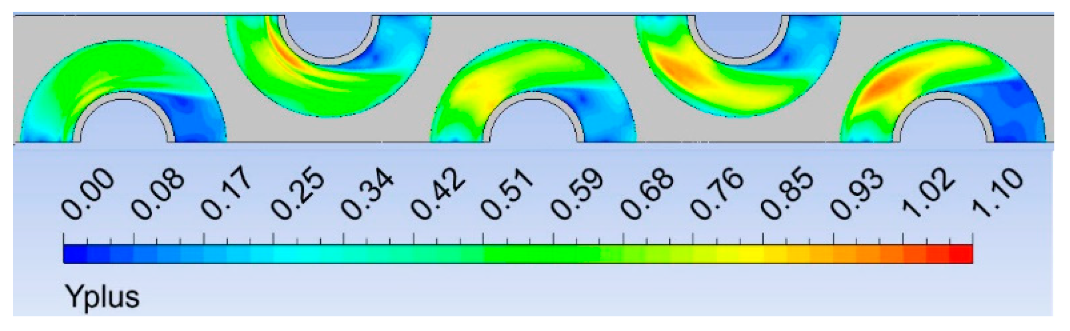
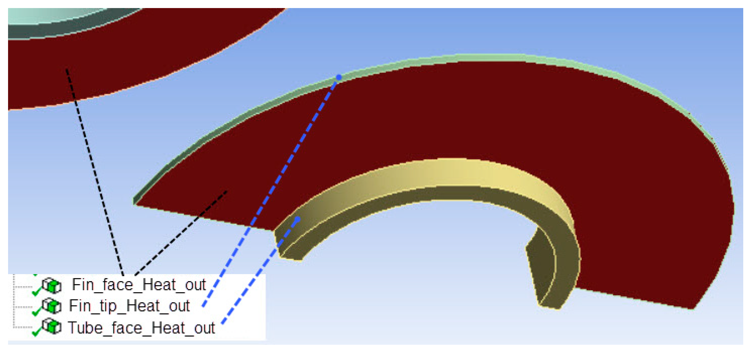
3.1.1. Mathematical Model

The numerical domain was chosen to perform the numerical analysis of the tube heat exchanger. For a heat exchanger with a uniform fluid flow field at the inlet, a typical repeating section in the heat exchanger is selected for the domain (Figure 4), and the solutions obtained are assumed valid for the entire heat exchanger.

Discretization of the geometrical model form the final volume and the set of all finite volumes makes a geometry mesh. The computational mesh was created in ANSYS Meshing software by using a hybrid mesh where most of the volume is structured mesh and the smaller part around the fins is unstructured mesh. Among different tested turbulence models, the k-ω SST model of turbulence with steady-state fluid flow and heat transfer was selected [18] because the results of numerical experiments show that the k-ω SST engineering turbulence model accurately captures the turbulent flow behaviour in the inner and outer regions of the boundary layer for wide range of engineering problems [19]. Second order solvers were used with residuals convergence limit 10⁻⁴ for all solved equations except the energy equation for which the criterion was set to 10⁻⁹. The final mesh, which gives results independent of the numeric mesh consists of approximately 11 million control volumes, where dimensionless wall distance y+ < 1 (Figure 5, Figure 6 and Figure 7).

Details related to the convergence criteria, numerical simulation parameters and the validation of results obtained are presented in [20]. The boundary conditions were defined according to

Table 3. Boundary conditions for Computational fluid dynamics simulations.

Inlet Air Temperature	K	288
Air velocity at the inlet of the heat exchanger	m/s	1, 2, 3, 5, 7
Inlet air turbulence intensity	%	5
Internal tube wall temperature	K	353
Outlet air pressure	Pa	101,325
Wall condition		Hydraulically smooth wall

.

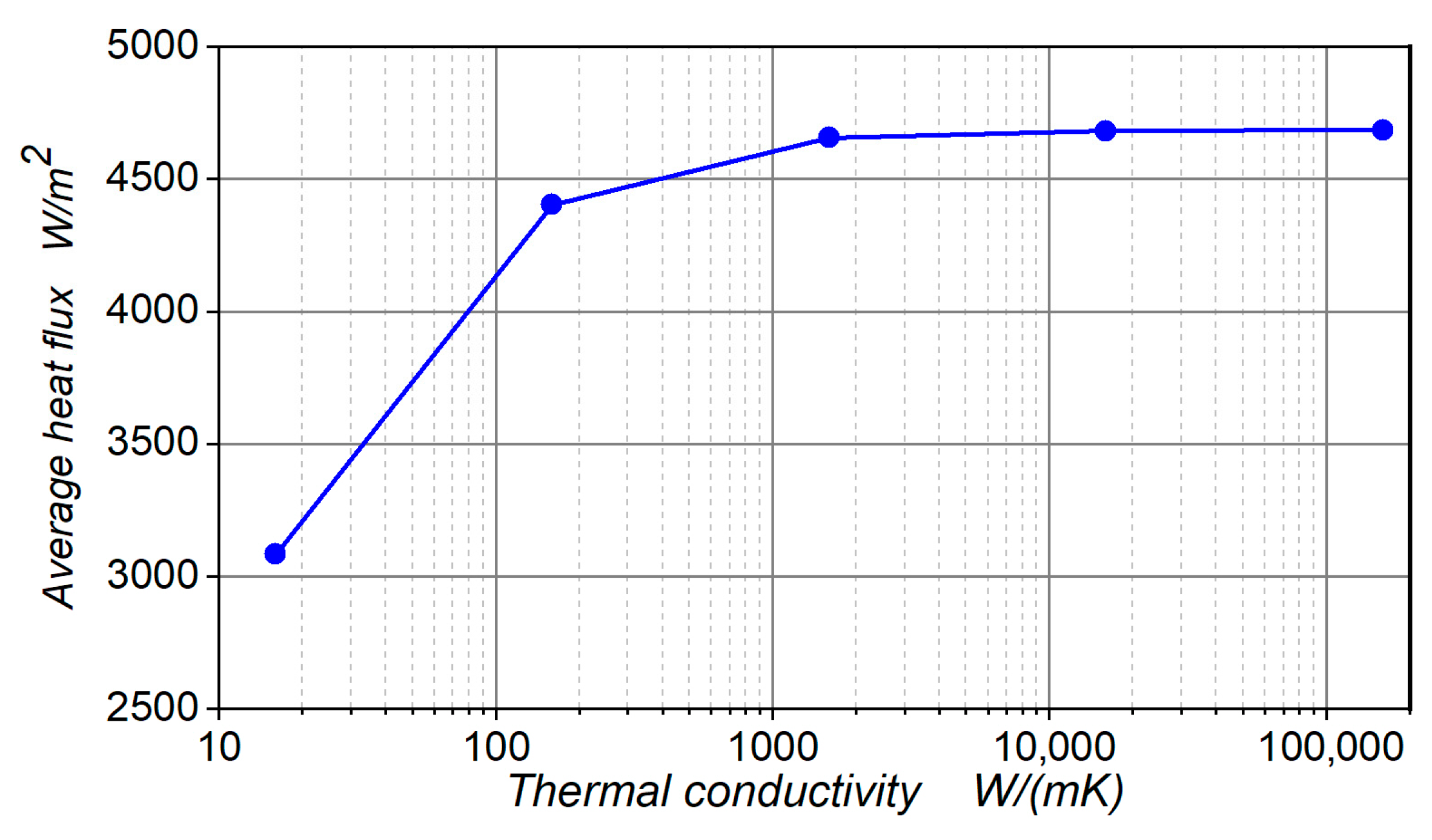
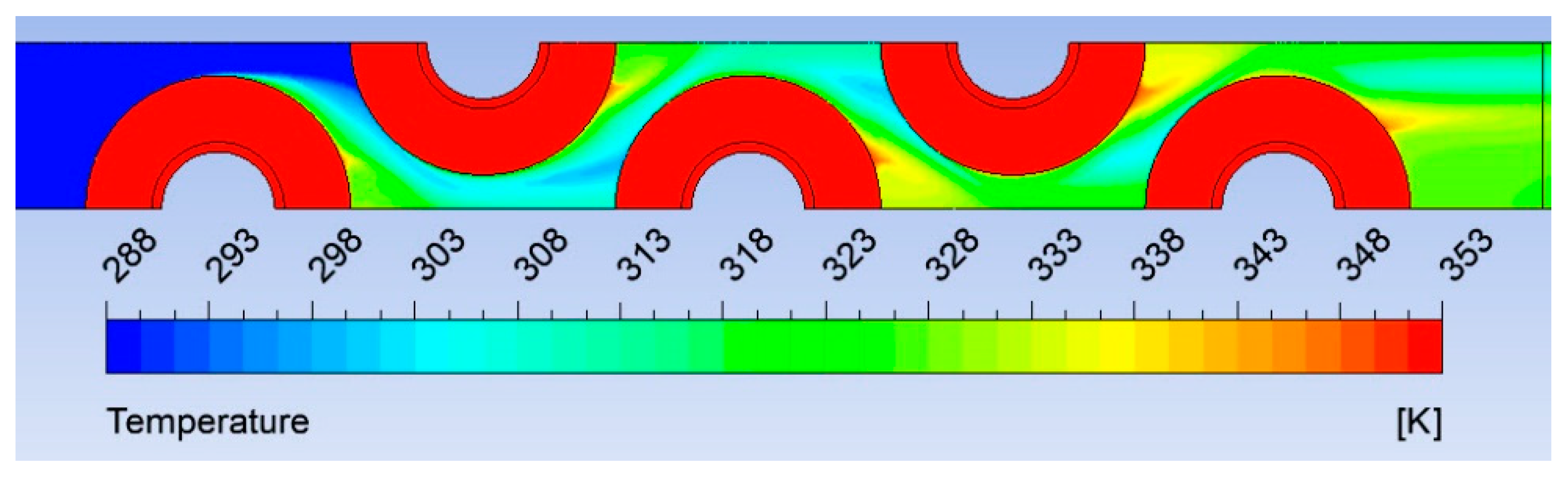
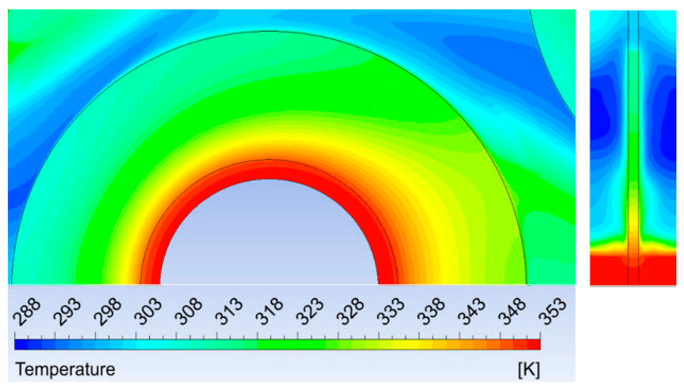
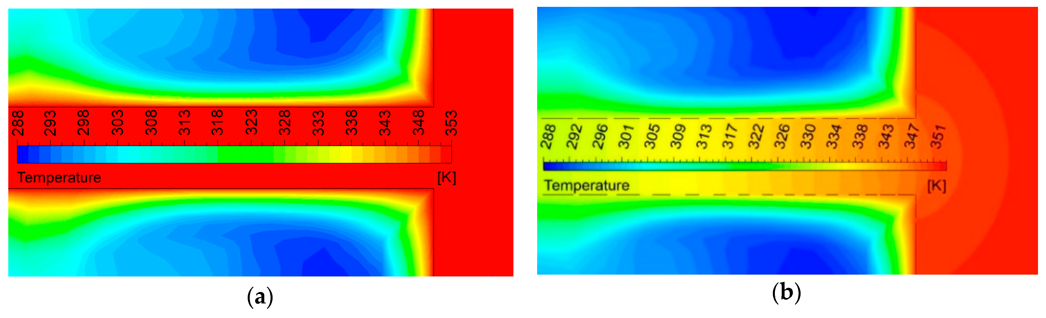
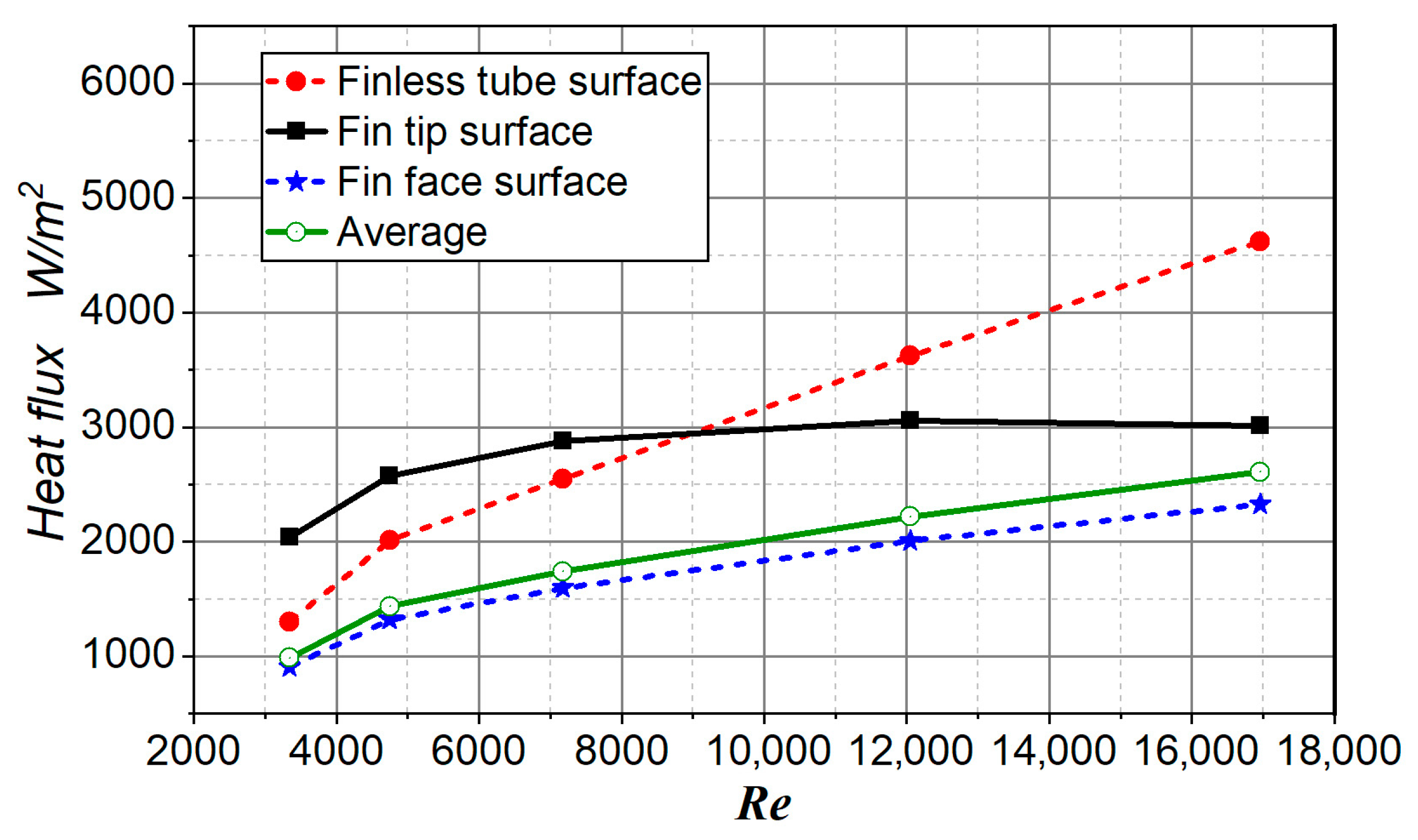
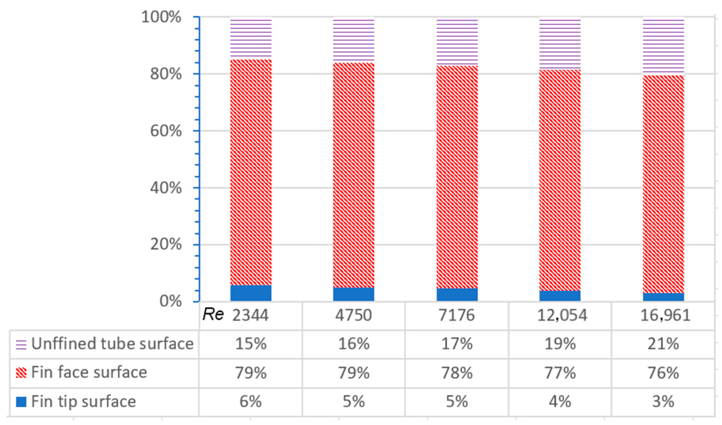
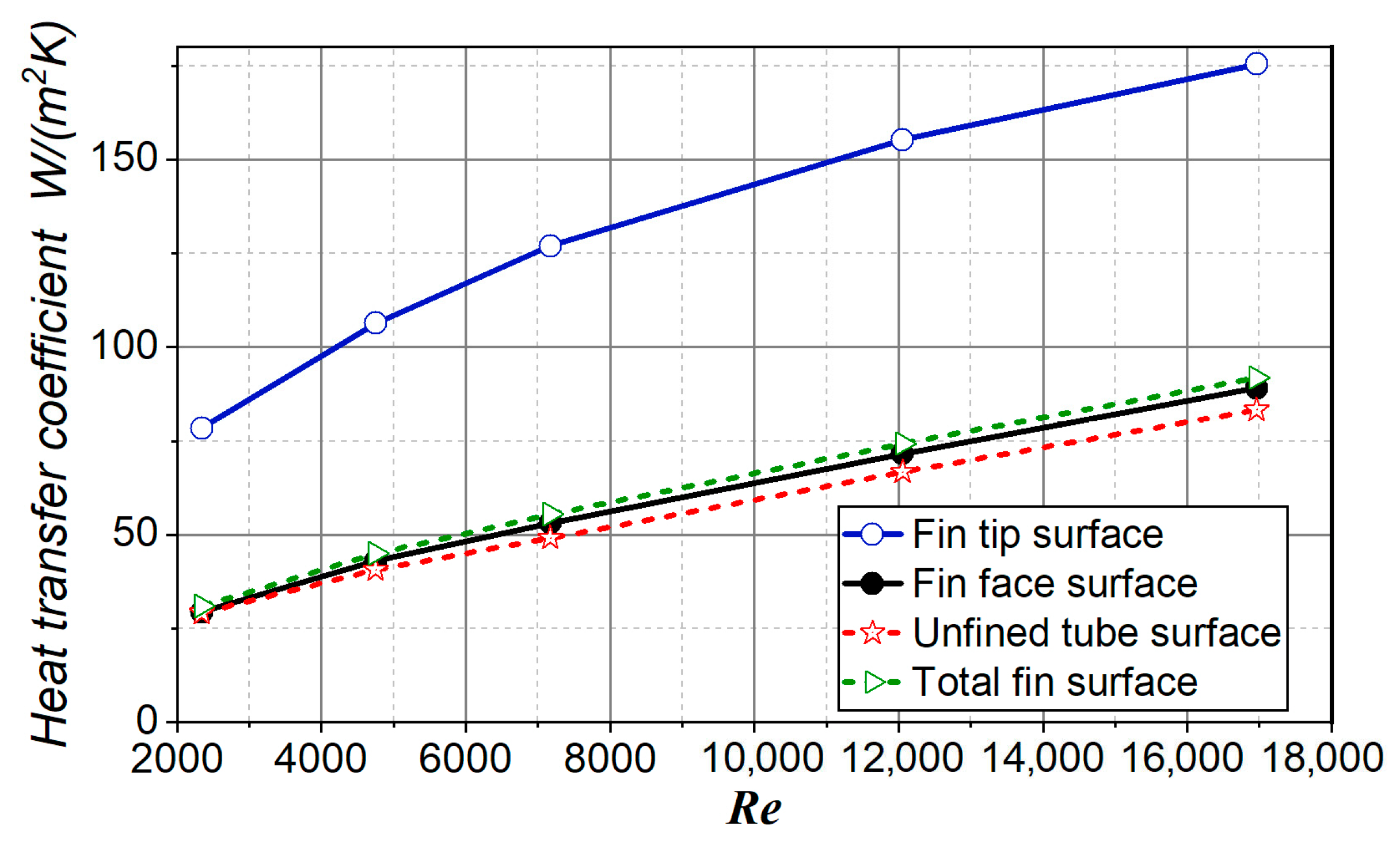
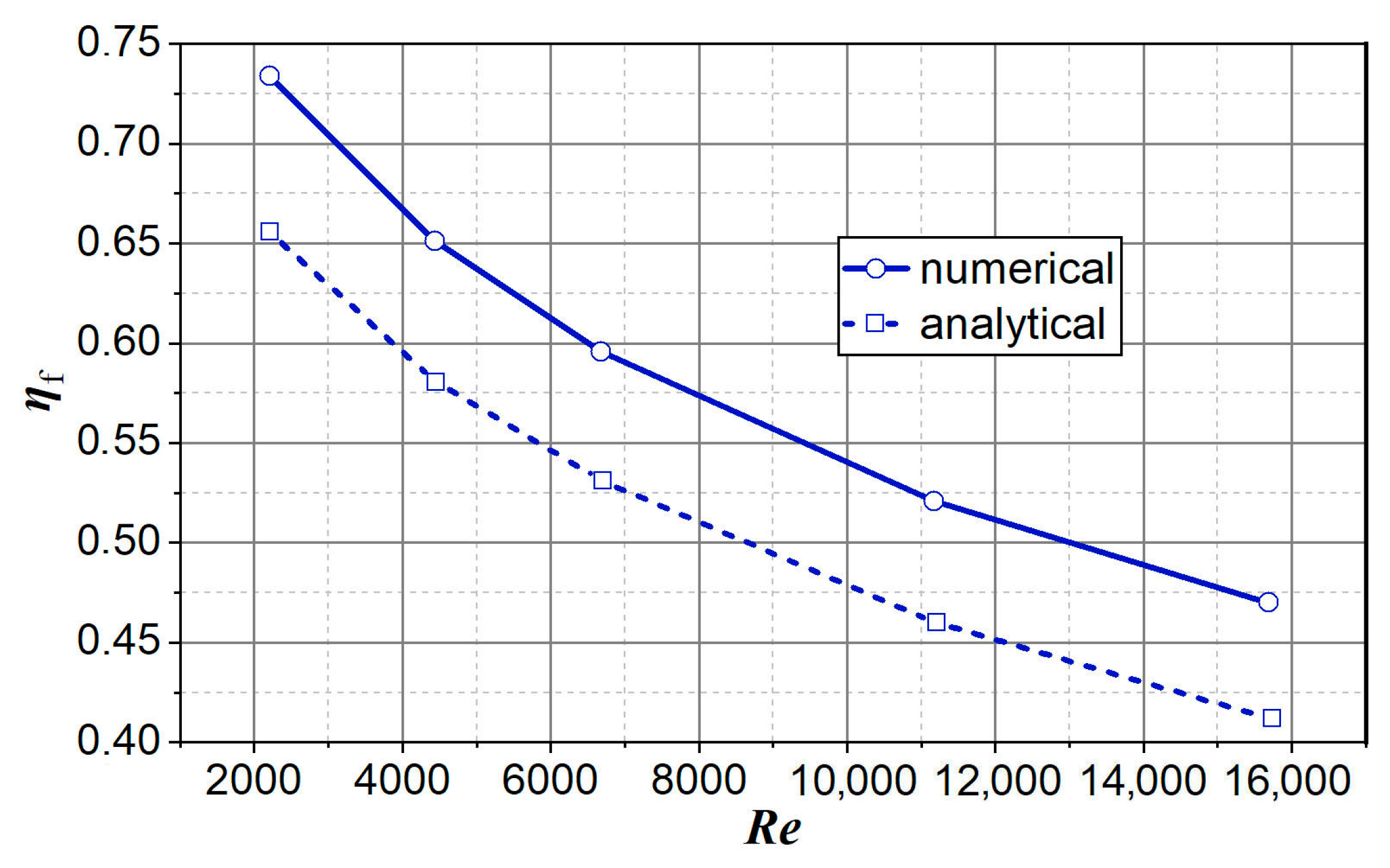
3.1.2. Numerical Simulation Results

With the aim to simulate an ideal fin with infinite thermal conductivity, the influence of the thermal conductivity to the average heat flux was investigated. This influence was numerically analysed by setting five values of thermal conductivity (16 W/(mK), 160 W/(mK), 1600 W/(mK), 16,000W/(mK), 160,000 W/(mK)) at an air velocity of 5 m/s (Re = 11,218).

It can be seen from Figure 8 that by taking a value of 16,000 W/(mK) for thermal conductivity of the fin material, it is possible to simulate the infinite fin heat conductivity with sufficient accuracy because the difference in heat flux compared to the thermal conductivity of 160,000 W/(mK) is less than 0.06%. To make the calculation error even smaller, the thermal conductivity of 160,000 W/(mK) is chosen for further calculation. A numerical simulation for the case of infinite thermal conductivity was performed for both types of fins. Five airflow rates were chosen (see Table 2). In order to be able to analyse in detail the heat transfer on particular fin surfaces, the named selection for face surfaces of the fin, the fin tip surface and the face surface of the unfinned part of tubes are defined (Figure 9).

In the case of infinite thermal conductivity (Figure 10), the entire fin surface temperature is close to the temperature of the fin base surface.

After that, numerical simulation for stainless steel (thermal conductivity of 16 W/(mK)) was performed for defined airflow rates. For a finite conduction resistance, a temperature gradient must exist along the fin. For stainless steel, the temperature variation in the longitudinal direction (Figure 11, left) is important. The temperature difference in the transverse section of the fin is small compared to the difference between the temperature of the fin surface and the environment as it is initially assumed for the thin fins (Figure 11, right). This can be checked by Biot (Bi) number which is in this case 0.0009 (<< 0.1). In addition, the temperature distribution across a fin surface area is not uniform (Figure 11, left).

Therefore, due to the turbulent flow conditions in the fin sections, the heat transfer coefficient at the surface area is not constant. The assumption of a uniform heat transfer coefficient along the surface area of the fins can result in a fin efficiency difference relative to actual values up to 40% [21]. The local characteristics of the temperature field according to Figure 12b show that in the area of the fin base surface, the temperature is lower than in the tube area between the fins, so for the first row of tubes, it is 348 K.

The amount of temperature drop in the fin base surface depends on the ratio h/t_f [15]. The presence of the fin, in addition to depressing its own base temperature, also depresses the temperature of the adjacent tube material, thereby slightly reducing the heat transfer from the unfinned tube wall. It can be seen that the assumption of a uniform base fin temperature equal to the temperature of the unfinned tube surface area can lead to significant errors in the calculated heat transfer rates from the fins [22]. An increase in the wall thickness increases the error. Heat flux is different on each surface. Figure 13 shows the heat flux on annular fin surfaces. The heat flux on the fin tip surface is much bigger than on the fin face surface. In addition, this indicates that the convective heat transfer on the fin tip surface is much bigger than on the fin face surface.

Figure 14 shows the share of the heat rate on particular surfaces in the total heat rate for annular fins for different Re numbers.

The mass average is used to calculate individual airflow variables at certain boundaries (e.g., at the inlet and outlet of the heat exchanger). In ANSYS CFD-Post, the appropriate function is massFlowAve. This function is defined by the expression:

$$massFlowAve(\varphi )=\frac{{\displaystyle \sum (\dot{m}\varphi )}}{{\displaystyle \sum \dot{m}}}.$$

(34)

The variable $\varphi$ represents the fluid flow variable that is being observed and $\dot{m}$ is the local mass flow rate. Each member of the sum is taken at the node level of the observed section. The average air temperature in the heat exchanger (the reference temperature) is defined by the expression:

$$T_2=\frac{T_{\mathrm{in}}-T_{\mathrm{out}}}{2}.$$

(35)

The average temperatures of the named surfaces were obtained from ANSYS Fluent using the areaAve function (

Table 4. Average temperature of fin surfaces.

Air Velocity (m/s)	Fin Face Surface Temperature (K)	Fin Tip Surface Temperature (K)	Total Fin Surface Temperature (K)	Outer Unfinned Tube Surface Temp. (K)
1	338.8	333.8	338.6	352.4
2	333.4	326.8	333.2	352.1
3	330.0	322.7	329.8	351.9
5	325.3	316.9	325.0	351.5
7	321.9	313.0	321.6	351.3

). The area-weighted average of a quantity is computed by dividing the summation of the product of the selected field variable and facet area by the total area of the surface:

$$areaAve(\varphi )=\frac{{\displaystyle \sum {\varphi }_{\mathrm{i}}}{A}_{\mathrm{i}}}{A}.$$

(36)

Figure 15 shows the convective heat transfer coefficient on particular fin surfaces.

The convective heat transfer coefficient was calculated on the basis of numerical simulation data. Data of the average temperature of a given surface area, the heat rate on this surface and the amount of surface area were taken. For example, the convective heat transfer coefficient for the fin face surface is calculated according to the Equation (37):

$${\alpha }_{\mathrm{f},\mathrm{f}}=\frac{{\dot{Q}}_{\mathrm{f},\mathrm{f}}}{A_{\mathrm{f},\mathrm{f}}(T_{\mathrm{f},\mathrm{f}}-T_2)}.$$

(37)

4. Discussion

Based on the numerically obtained results for the heat transfer rate ${\dot{Q}}_{\mathrm{f}}$ and ${\dot{Q}}_{\mathrm{f},\max }$ using Equation (11), the efficiency of the fin η_f is calculated. An analytically calculated theoretical value of the fin efficiency η_f,th is calculated according to Equation (24) and then the corrected theoretical value of the fin efficiency η_f is calculated according to Equation (29). Figure 16 shows that the analytically calculated fin efficiency is smaller than the numerically obtained one. This is the consequence of introducing simplifications in the analytical derivation of the equation for the fin efficiency. The difference in efficiency varies from 10.7% to 12.5% for lower and higher Re numbers, respectively. The overall surface efficiency η_o is calculated according to Equation (19) based on the numerically obtained results for the heat transfer rate $\dot{Q}$ and ${\dot{Q}}_{\max }$. Analytically, η_o is calculated according to Equation (22), where η_f is also analytically obtained.

Figure 17 shows that the analytically calculated overall surface efficiency is smaller than that obtained numerically. This is related to the error in the calculation of the analytical fin efficiency and the application of Equation (18) in which the assumption ${\alpha }_{\mathrm{t}}\approx {\alpha }_{\mathrm{f}}$ is embedded. The difference in numerical and analytical efficiencies for annular fins is 11.6% to 10.9% for lower and higher Re numbers, respectively.

The convective heat transfer coefficient can also be calculated based on data of numerical simulation according to Equation (38):

$${\alpha }_{\mathrm{f},\mathrm{n}}=\frac{\dot{Q}}{{\eta }_{\mathrm{o}}\left(A_{\mathrm{t}}+A_{\mathrm{f}}\right)(T_{\mathrm{f}}-T_2)}.$$

(38)

Figure 18 shows that the convective heat transfer coefficient based on the data obtained by numerical analysis is smaller than that calculated according to Equation (30). This is in accordance with the experimental results. The difference varies from 23.2% to 18.5% for lower and higher Re numbers, respectively.

As mentioned above, the concept of the adiabatic fin tip introduces some error in calculation. The amount of error can be estimated according to:

$$Error=\frac{\left(Q_{\mathrm{f}}-Q_{\mathrm{f},\mathrm{a}}\right)}{Q_{\mathrm{f}}}\cdot 100\%,$$

(39)

$$Q_{\mathrm{f},\mathrm{a}}=\mathsf{\Delta }{A}_{\mathrm{f}}\cdot q_{\mathrm{f},\mathrm{f}}+Q_{\mathrm{f},\mathrm{f}},$$

(40)

$$\mathsf{\Delta }{A}_{\mathrm{f}}=\left(r_{2\mathrm{c}}^2-r_{\mathrm{o}}^2\right)\frac{\pi }{2}-\left(r_2^2-r_{\mathrm{o}}^2\right)\frac{\pi }{2}.$$

(41)

Figure 19 shows that the amount of error ranges from 2.5% to 5.4% for the ratio t_f/h_f = 0.05 and 2000 < Re < 17,000. In order to take into account the higher convection at the fin tip and reduce error, our recommendation is to take higher amounts than t_f/2, which is recommended in the literature.

Good results can be obtained by for Re numbers up to 16,000:

$$h_{\mathrm{e}}=h_{\mathrm{f}}+1.5\cdot t_{\mathrm{f}},$$

(42)

and for Re numbers over 16,000:

$$h_{\mathrm{e}}=h_{\mathrm{f}}+t_{\mathrm{f}}.$$

(43)

The increase in h_e reduces the fin efficiency to some extent.

5. Conclusions

Fin efficiency analysis was carried out with the aim of determining the error occurring when applying the commonly used equation in the literature for the efficiency of the annular fin. Stainless steel was selected as the fin material because it has lower thermal conductivity than other applied materials, thus the error is more pronounced. For the analysed interval of Re numbers from 2000 to 17,000, it was found that the application of analytical expressions for annular fins gives a fin efficiency coefficient of less than 10.7% to 12.6% compared to numerical analysis results. Related to these, the results for the efficiency coefficient of the entire surface are 11.6% to 10.9% lower compared to the results obtained by numerical analysis. At the same time, the convective heat transfer coefficient determined by numerical analysis is 23.2% to 18.5% lower than that calculated by using analytical terms.

The reasons for these deviations are the assumptions and simplifications introduced when deriving analytic expressions. The greatest impact on the amount of error is the assumption of equal temperature of the fin base surface and the outer surface of the tube, which neglects the temperature drop on the base surface of the fin. Also, the model of the adiabatic fin tip does not consider the higher heat flux at the fin tip compared to the fin face surface. The above-mentioned errors have opposing signs, so the overall effect is about 20% for annular fins. This should be considered when sizing the heat exchanger and one should increase the heat exchanger surface by the appropriate amount. In addition, corrected fin height is recommended for the analysed range of Re numbers.

References

1. Harper, D.R.; Brown, W.B. Mathematical equations for heat conduction in the fins of air cooled engines. NACA R 1922, 158, 32. [Google Scholar]
2. Murray, W.M. Heat transfer through an annular disk or fin of uniform thickness. Trans. ASME J. Appl. Mech. 1938, 60, A78–A81. [Google Scholar]
3. Gardner, K.A. Efficiency of extended surface. Trans. ASME 1945, 67, 621. [Google Scholar]
4. Darvishi, M.T.; Khani, F.; Aziz, A. Numerical investigation for a hyperbolic annular fin with temperature dependent thermal conductivity. Propuls. Power Res. 2016, 5, 55–62. [Google Scholar] [CrossRef]
5. Ghai, M.L. Heat transfer in straight fins. In Proceedings of the General Discussion on Heat Transfer, London, UK, 11–13 September 1951. [Google Scholar]
6. Zaidan, M.H.; Alkumait, A.A.R.; Ibrahim, T.K. Assessment of heat transfer and fluid flow characteristics within finned flat tube. Case Stud. Therm. Eng. 2018, 12, 557–562. [Google Scholar] [CrossRef]
7. Nemati, H.; Moghimi, M. Numerical study of flow over annular-finned tube heat exchangers by different turbulent models. CFD Lett. 2014, 6, 101–112. [Google Scholar]
8. Look, D.C., Jr.; Krishnan, A. One-dimensional fin-tip boundary condition correction II. Heat Transf. Eng. 2001, 22, 35–40. [Google Scholar] [CrossRef]
9. Nemati, H.; Samivand, S. Performance optimization of annular elliptical fin based on thermo-geometric parameters. Alexandria Eng. J. 2015, 54, 1037–1042. [Google Scholar] [CrossRef]
10. Chen, H.L.; Wang, C.C. Analytical analysis and experimental verification of trapezoidal fin for assessment of heat sink performance and material saving. Appl. Therm. Eng. 2016, 98, 203–212. [Google Scholar] [CrossRef]
11. Lane, H.J.; Heggs, P.J. Extended surface heat transfer-the dovetail fin. Appl. Therm. Eng. 2005, 25, 2555–2565. [Google Scholar] [CrossRef]
12. Cléirigh, C.T.Ó.; Smith, W.J. Can CFD accurately predict the heat-transfer and pressure-drop performance of finned-tube bundles? Appl. Therm. Eng. 2014, 73, 679–688. [Google Scholar] [CrossRef]
13. Incropera, F.P.; DeWitt, D.P.; Bergman, T.L.; Lavine, A.S. Fundamentals of Heat and Mass Transfer; John Wiley & Sons, Inc.: Hoboken, NJ, USA, 2007. [Google Scholar]
14. Kraus, A.D.; Aziz, A.; Welty, J. Extended Surface Heat Transfer; John Wiley & Sons, Inc.: Hoboken, NJ, USA, 2001. [Google Scholar]
15. Sparrow, E.M.; Hennecke, D.K. Temperature depression at the base of a fin. Trans. ASME 1970, 92, 204–206. [Google Scholar] [CrossRef]
16. Sparrow, E.M.; Lee, L. Effects of fin base temperature depression in a multifin array. J. Heat Transf. 1975, 97, 463–465. [Google Scholar] [CrossRef]
17. Hashizume, K.; Morikawa, R.; Koyama, T.; Matsue, T. Fin efficiency of serrated fins. Heat Transf. Eng. 2002, 23, 7–14. [Google Scholar] [CrossRef]
18. Taler, D. Numerical Modelling and Experimental Testing of Heat Exchangers; Springer: Berlin, Germany, 2019; Volume 161. [Google Scholar]
19. Könözsy, L. Volume I: Theoretical background and development of an anisotropic hybrid k-omega shear-stress transport/stochastic turbulence model. In A New Hypothesis on the Anisotropic Reynolds Stress Tensor for Turbulent Flows; Springer: Berlin, Germany, 2019; Volume 120. [Google Scholar]
20. Bošnjaković, M.; Čikić, A.; Muhič, S.; Stojkov, M. Development of a new type of finned heat exchanger. Tehnical Gazette 2017, 24, 1785–1796. [Google Scholar] [CrossRef]
21. Huang, L.J.; Shah, R.K. Assessment of calculation methods for efficiency of straight fins of rectangular profile. Int. J. Heat Fluid Flow 1992, 13, 282–293. [Google Scholar] [CrossRef]
22. Suryanarayana, N.W. Two-dimensional effects on heat transfer rates from an array of straight fins. J. Heat Transf. 1977, 99, 129–132. [Google Scholar] [CrossRef]
Figure 1. Characteristic dimensions of the finned surface.
Energies 12 01787 g001
Figure 2. The periodic temperature profile in the tube wall.
Energies 12 01787 g002
Figure 3. Adiabatic fin tip assumption.
Energies 12 01787 g003
Figure 4. Schematic view of the computational domain.
Energies 12 01787 g004
Figure 5. Nu dependence on the number of control volumes.
Energies 12 01787 g005
Figure 6. Eu dependence on the number of control volumes.
Energies 12 01787 g006
Figure 7. Dimensionless wall distance y+.
Energies 12 01787 g007
Figure 8. Heat flux versus fin thermal conductivity.
Energies 12 01787 g008
Figure 9. The named selection of fin.
Energies 12 01787 g009
Figure 10. Temperature contours of ideal annular fins.
Energies 12 01787 g010
Figure 11. Temperature contours over fins in the 3rd row for air velocity 5 m/s. Left: Finned tube cross section, Right: Fin cross-section.
Energies 12 01787 g011
Figure 12. Fin temperature contours: (a) Temperature contour at λ = 16,000 W/(mK). (b) Temperature contour at λ = 16 W/(mK).
Energies 12 01787 g012
Figure 13. Heat flux on annular fin surfaces.
Energies 12 01787 g013
Figure 14. The share of heat rate on particular surfaces of the annular fin.
Energies 12 01787 g014
Figure 15. Convective heat transfer coefficient.
Energies 12 01787 g015
Figure 16. The efficiency of fins determined numerically and analytically.
Energies 12 01787 g016
Figure 17. The overall surface efficiency ηo determined numerically and analytically.
Energies 12 01787 g017
Figure 18. Convective heat transfer coefficient based on numerical analysis data and analytical calculation.
Energies 12 01787 g018
Figure 19. Error for adiabatic fin tip concept.
Energies 12 01787 g019