Hybrid AC/DC Microgrid Planning with Optimal Placement of DC Feeders

Abstract

With the significant increase in DC loads (such as data and telecommunication centers) at the power distribution level, an additional set of power electronic converters are required to connect these DC loads to the AC-dominant power network. Notably, hybrid AC/DC microgrids (MGs) serve as promising solutions to satisfying both the AC and DC loads with a reduced number of installed converters. Since DC loads may be randomly distributed in the MG, how to place DC feeders to simultaneously fulfill the economic and security requirements of MG operations remains a challenging problem. To address this issue, this paper proposes a hybrid AC/DC MG planning model to determine the optimal placement of DC feeders with the objective of minimizing the total cost of the investment of distributed energy resources (DERs), converters, and AC/DC distribution lines, as well as the operation of DERs. In particular, the power flow of the hybrid AC/DC MG is derived in a unified manner and then incorporated in the planning model. Eventually, the proposed model suffices to find the optimal number and siting for both DERs and DC feeders while ensuring the continuality of the DC feeders. The proposed model is tested in two MG-based distribution systems, and its effectiveness is validated by the results of numerical experiments.

1. Introduction

A microgrid (MG) is a small-scale localized power system mainly composed of distributed energy resources (DERs), loads, converters, as well as monitoring and protection devices. According to the power supply mode of the internal network, MGs can be divided into AC MGs, DC MGs and hybrid AC/DC MGs. Compared with most common AC MGs, DC MGs feature less power losses due to the direct connection of DC-based sources and loads to DC buses [1]. When connected to the utility grid, DC MGs however need to rely on inverters with a large capacity at their common points of coupling. Besides, the connection of AC-based sources and loads necessitates additional AC-DC converters in a DC MG, which introduces unavoidable power losses in the conversion process. Accordingly, a hybrid AC/DC MG presents a more economic and flexible solution to integrate both AC- and DC-based DERs and loads within clearly defined electrical boundaries. A typical AC/DC hybrid MG is shown in Figure 1. A variety of DERs (such as energy storage systems (ESSs), wind turbines (WTs), photovoltaic arrays (PVs), diesel generators, micro turbines (MTs)) and AC loads and DC loads) are interfaced with AC or DC buses through pertinent converters. Such a hybrid network configuration effectively combines the advantages of AC and DC MGs to improve the efficiency, flexibility, and sustainability of electricity provisions. However, how to deploy DERs and AC/DC network components simultaneously in a hybrid AC/DC MG remains a challenging task.

Given that the research on MGs keeps burgeoning, most of the existing studies focus on the planning or operation of AC MGs with the goal of minimizing the total amount of investment, operation costs and pollutant emissions while maximizing the reliability of electricity services [2]. There also exist some studies on DC MGs. For example, references [3,4,5,6] devote their attention to modelling the planning and sizing of DC MGs. In [3], a new energy storage configuration comprising photovoltaic battery systems, a series of DC electric springs and a noncritical load is proposed to reduce the required capacity of batteries in a DC MG. Reference [4] develops a planning framework for optimally configuring low-power low-voltage DC MGs in order to minimize the upfront cost associated with photovoltaic systems. Reference [5] optimizes the investment of PVs, WTs and ESSs in a DC MG based on the changing the capital cost. A non-dominated sorting genetic algorithm is implemented in reference [6] to solve the multi-objective optimal sizing problem with the goal of achieving a trade-off between the cost and the reliability of DC MG operations. Another group of works [7,8,9] focus on the operation of DC MGs. Reference [7] proposes three new operation strategies such that a set of DC MGs in distribution systems can cooperate on pursuing specified objectives: loss reduction, full unbalance compensation, and partial unbalance compensation. In reference [8], a multi-level energy management system (EMS) is proposed for DC MG operations. Reference [9] studies the planning and operation of standalone DC MGs in rural and urban settings with detail comparisons of various cost components, electrical productions, energy management and emissions.

In comparison, the research on hybrid AC/DC MG is still at the very beginning. There have been only a few studies on the energy management of these hybrid MGs. In [10], an autonomous power management scheme is proposed to model the accurate loading condition of a DC MG before importing power from an interlinked AC MG. The proposed scheme not only enables the voltage regulation in the DC MG but also reduces the number of converters required in operation. In [11], an energy management and operation model of a hybrid AC/DC MG is proposed, which is by nature a mixed integer linear problem that seeks to minimize the total operation cost in a 24-hour period by considering the interconnection of AC and DC sub grids. Some studies take the uncertainty of renewable energy into consideration. For example, reference [12] proposes a stochastic optimization framework for the optimal operation and management of hybrid AC/DC MGs in the presence of renewable energy sources and storage devices. Reference [13] develops a robust dispatch model for AC/DC hybrid MGs under uncertainty. Only a limited number of papers focus on the planning of hybrid AC/DC MGs. The authors of [14,15] performed some interesting explorations into this topic. Reference [14] presents a MG planning model to determine the optimal size and generation mix of DERs, along with the MG type (i.e., AC or DC). Reference [15] further proposes an hybrid AC/DC MG planning model with the objective of minimizing the total MG planning cost. The only shortcoming is that the power flow is not taken into account. Reference [16] proposes a novel stochastic planning model for hybrid AC/DC distribution systems, and the power flow is adequately considered. However, the AC/DC distribution line investment costs are ignored. The employed genetic algorithm would not necessarily lead to a global optimum.

This paper aims to improve on the existing literature by considering the power flow and distribution line investment, and formulate the problem into a tractable form with a global optimum. However, the tractable form of the hybrid AC/DC power flow remains a challenge. Regarding this problem, several studies have examined the DC power flow or hybrid AC/DC power flow in DC or AC/DC systems. In [17], a classic Newton’s method and an approximated Newton’s method are applied in the master-slave and island (with droop controls) operation modes, respectively. In [18], an optimal power flow of DC MGs by employing the second-order cone programming-based convex relaxation which only relies on the assumptions of uniform nodal voltage upper bounds and positive network losses is investigated. In reference [19], optimal AC and DC power flows are modeled separately without considering their potential hybrid connection. Reference [20] presents a semidefinite relaxation method to approach the optimal power flow for AC/DC grids, and the method is proved to be effective. Reference [21] develops a hybrid AC/DC optimal power flow model based on second order cone relaxation approach, the effectiveness of which is verified by the results of numerical experiments.

In all, there have been several studies proposing optimization models for planning and operating either AC or DC MGs, but research achievements in the planning or operation of hybrid AC/DC MGs remain insufficient. In particular, the physical settings (e.g., the implementation of AC or DC buses/lines) of a MG are pre-specified and unchanged in those existing studies, which however present immense opportunities for constant improvement in MG operation performance in practice (e.g., flexible network configurations). Furthermore, power flow constraints, which may affect the placement of DERs, are commonly ignored in the prevalent decision-making process. This paper follows [15] but improves it by considering more fine-grained technical and operational restrictions in the planning of hybrid AC/DC MGs. To sum up, the main contributions of this paper may be listed as follows:

(1)

A comprehensive optimization model is proposed for planning hybrid AC/DC MGs. The model, which is eventually converted into a mixed integer second order cone programming (MISOCP) or mixed integer linear programming (MILP) problem, not only considers the investment and operation cost of DERs, but also considers the investment cost of different types of converters and distribution lines in a hybrid AC/DC MG.

(2)

A hybrid AC/DC power flow model is presented for modeling the operation of hybrid AC/DC MGs in a high-fidelity manner. Based on the DistFlow model, AC and DC power flows are unified and incorporated in the optimization model of hybrid AC/DC MG operations.

(3)

A practical strategy is developed to optimally place the DC feeders. The strategy uses binary variables to describe the AC/DC type of branches and buses while maintaining the continuity of DC feeders.

The remainder of this paper is organized as follows. The proposed models are presented in Section 2. Moreover, case studies are provided in Section 3. Finally conclusions are demonstrated in Section 4.

2. Proposed Hybrid MG Planning Model

In this section, a basic hybrid AC/DC MG planning model is formulated firstly after taking into account the costs of both converters and AC/DC distribution lines. Then a set of hybrid AC/DC power flow constraints are introduced and integrated into the basic model. Furthermore, we extend the model by exploring the possibility of forming DC feeders that are originated from the main AC network (as shown in Figure 2). Finally, some techniques are employed to convert the extended model into a MISOCP problem.

It should be noted that the model is established based on the assumption that DC loads share the same voltage with the DC feeders. In other words, the DC loads can directly use the voltage level of the DC feeders and no DC/DC converters are needed. According to [22], most of the existing interconnected DC distribution systems are data centers (380 V), telecommunication power systems (48 V), traction power systems (600 V, 750 V or even up to 1 kV), and experimental setups (230 V, 380 V and 325 V). In this regard, we consider the studied DC loads are either data centers and experimental setups about 380 V or traction power systems about 750 V. Accordingly, the DC feeders are either about 380 V or 750 V. With respect to other DC loads such as computers, laptops, microwave ovens and lighting, they are randomly distributed in the distribution system and only take a small amount of the loads. Thus they are considered as integrated AC loads and not taken into account into the studied DC loads.

2.1. Basic Hybrid AC/DC MG Planning Model

As for MG planning, the most common concern is related to their economics. The total cost of implementing a MG includes the investment cost and operation cost of DERs, and the investment cost of converters and AC/DC distribution lines. Therefore, the objective of the hybrid AC/DC MG planning problem, as formulated in (1), is to minimize the overall investment and operation cost (including the DER investment cost, the converter investment cost, the distribution line investment cost, and the MG operation cost) throughout the life cycle. Since the life cycle of a MG lasts for decades, the total cost is calculated in terms of the present-worth value.

$$f=\min DC+CC+LC+OC$$

(1)

$$\begin{array}{cc}\hfill DC=& {\displaystyle \sum _{i\in \mathcal{G}}{K}_i^g{I}_i^g{\overline{P}}_i^g{x}_i^g}+{\displaystyle \sum _{i\in \mathcal{B}}{K}_i^b(I{P}_i^b{\overline{P}}_i^b+I{E}_i^b{\overline{E}}_i^b)x_i^b}+\hfill \\ & {\displaystyle \sum _{i\in \mathcal{W}}{K}_i^w{I}_i^w{\overline{P}}_i^w{x}_i^w}+{\displaystyle \sum _{i\in \mathcal{V}}{K}_i^v{I}_i^v{\overline{P}}_i^v{x}_i^v}\hfill \end{array}$$

(2)

$$\begin{array}{cc}\hfill CC=& {\displaystyle \sum _{i\in \mathcal{G}}{\displaystyle \sum _{j\in \mathcal{N}}{K}_i^{g,c}{I}_i^{g,c}{\overline{P}}_i^g{x}_{ij}^g{y}_j^d}}+{\displaystyle \sum _{i\in \mathcal{B}}{\displaystyle \sum _{j\in \mathcal{N}}{K}_i^{b,c}{I}_i^{b,c}{\overline{P}}_i^b{x}_{ij}^b{y}_j^a}}+\hfill \\ & {\displaystyle \sum _{i\in \mathcal{W}}{\displaystyle \sum _{j\in \mathcal{N}}{K}_i^{w,c}{I}_i^{w,c}{\overline{P}}_i^w{x}_{ij}^w{y}_j^d}}+{\displaystyle \sum _{i\in \mathcal{V}}{\displaystyle \sum _{j\in \mathcal{N}}{K}_i^{v,c}{I}_i^{v,c}{\overline{P}}_i^v{x}_{ij}^v{y}_j^a}}+\hfill \\ & {\displaystyle \sum _{j\in {\mathcal{N}}^a}{K}_{}^{ld,c,a}{\overline{P}}_j^{ld}{y}_j^d}+{\displaystyle \sum _{j\in {\mathcal{N}}^d}{K}_{}^{ld,c,d}{\overline{P}}_j^{ld}{y}_j^a+}\hfill \\ & {\displaystyle \sum _{(i,j)\in \mathcal{L}}{K}_{}^{li,c}{\overline{P}}_{ij}^{li}{z}_{ij}^{cp}}\hfill \end{array}$$

(3)

$$LC={\displaystyle \sum _{(i,j)\in \mathcal{L}}3K^{li,l}{I}_{ij}^{li}{z}_{ij}^a}+{\displaystyle \sum _{(i,j)\in \mathcal{L}}2K^{li,l}{I}_{ij}^{li}(z_{ij}^d+z_{ij}^{cp})}$$

(4)

$$OC={\displaystyle \sum _{d=1}^{365}{\displaystyle \sum _{h=1}^{24}\left\{{\displaystyle \sum _{i\in \mathcal{G}}{\rho }_i^g{p}_{idh}^g}+({\rho }_{dh}^{gd+}{p}_{dh}^{gd+}-{\rho }_{dh}^{gd-}{p}_{dh}^{gd-})\right\}}}$$

(5)

In the objective function (1), the investment cost in any future year is converted to the annual value at present by multiplying the present-worth coefficient as follows:

$$K_{\epsilon }=\frac{r{(1+r)}^{T_{\epsilon }^{}}}{{(1+r)}^{T_{\epsilon }^{}}-1}$$

(6)

where K_ε is the present worth coefficient of device ε; T_ε is the lifespan of device ε such as the DG, BS, PV, and WT in years; r is the interest.

The detailed DER investment cost is expressed as (2), where the first term is the investment cost of DGs such as MTs and diesel generators, the second term is the investment cost of battery storage systems (BSs), and the third and fourth terms represent the investment cost of WTs and PVs. The investment cost of DGs is assumed to be proportional to their capacity with the consideration of discounted costs. It should also be noted that the cost of investing BSs includes two parts: one is related to the capacity, while the other one depends on the maximum discharging power.

The investment cost of converters is shown as (3). The first term, which is proportional to the capacity of DGs, represents the converter investment cost of DGs. Only if the i-th DG is located at the j-th bus and the j-th bus is a DC bus (x^g_ij = 1 and y^d_j = 1), a AC/DC converter is needed for the AC-based DG. Otherwise, this part of cost is zero. Similarly, the second to the fourth terms represent the converter costs for BSs, WTs, and PVs, respectively. The fifth term represents the AC/DC converter cost for the AC load at the jth bus, which is also proportional to the maximum load at that bus. Similarly, the sixth term represents the DC/AC converter cost for the DC load at the j-th bus. The seventh term represents the AC/DC converter cost for DC feeders (which is proportional to the maximum capacity), where z^cp_ij is used to indicate the status of the coupling branch (i,j) between the AC network and DC network. In most cases, branch (i,j) is either a DC or AC branch, which means z^cp_ij = 0 and no converter cost is needed. However, if branch (i,j) is the coupling branch between AC and DC networks, z^cp_ij = 1 and a AC/DC converter is needed. The identification of the coupling branches will be detailed in the subsequent sections.

The investment cost of distribution lines is shown as (4). Each AC branch has three single-phase lines, while each DC branch has only two lines. Therefore, the first and second terms represent the investment cost of AC and DC distribution lines, respectively.

The operation cost of the MG over the year is expressed as (5). The generation costs of WTs and PVs are assumed to be zero as they consume no fuel. The first term is the fuel cost of DGs, while the second and third terms are related to the energy trading cost with the utility grid. Since the MG is assumed to either buy or sell power from or to the utility grid, the negative sign of the imported power means the MG feeds power back to the utility grid.

The MG operation cost is determined on a daily basis and then accumulated throughout the year. Considering the temporal correlation, several typical days instead of all days are considered in the simulation of MG daily operations for lessening the computational complexity of the optimization model.

The number of DGs, and that of BSs are subject to resource limits (7) and (8) (i.e., the maximum number constrained by the financial budgets). Similarly, the number of WTs or PVs is also subject to spatial and temporal restrictions (9) and (10):

$$0\le {\displaystyle \sum _{i\in \mathcal{G}}{x}_i^g}\le \left|\mathcal{G}\right|$$

(7)

$$0\le {\displaystyle \sum _{i\in \mathcal{B}}{x}_i^b}\le \left|\mathcal{B}\right|$$

(8)

$$0\le {\displaystyle \sum _{i\in \mathcal{W}}{x}_i^w}\le \left|\mathcal{W}\right|$$

(9)

$$0\le {\displaystyle \sum _{i\in \mathcal{V}}{x}_i^v}\le \left|\mathcal{V}\right|$$

(10)

As each DER can only be connected to one MG bus, the aggregated sum of pertinent location indicators should equal the deployment state of the DERs, as indicated in (11)–(14). If the i-th DER is connected to the j-th bus, then the location indicator associated with the jth bus is active and equal to 1; otherwise, all the indicators are inactive and equal to 0:

$$x_i^g={\displaystyle \sum _{j\in \mathcal{N}}{x}_{ij}^g}\forall i\in \mathcal{G}$$

(11)

$$x_i^b={\displaystyle \sum _{j\in \mathcal{N}}{x}_{ij}^b}\forall i\in \mathcal{B}$$

(12)

$$x_i^w={\displaystyle \sum _{j\in \mathcal{N}}{x}_{ij}^w}\forall i\in \mathcal{W}$$

(13)

$$x_i^v={\displaystyle \sum _{j\in \mathcal{N}}{x}_{ij}^v}\forall i\in \mathcal{V}$$

(14)

To avoid placing two and more DERs at a single bus, the following constraint (15) should be met:

$${\displaystyle \sum _{i\in \mathcal{G}}{x}_{ij}^g}+{\displaystyle \sum _{i\in \mathcal{B}}{x}_{ij}^b}+{\displaystyle \sum _{i\in \mathcal{W}}{x}_{ij}^w}+{\displaystyle \sum _{i\in \mathcal{V}}{x}_{ij}^v}\le 1\forall j\in \mathcal{N}$$

(15)

The power flow exchange with the utility grid is constrained by the maximum limits (16), while the power output of each DG is constrained by its lower and upper bound as (17).

$$0\le p_{dh}^{gd+},p_{dh}^{gd-}\le {\overline{P}}_{}^{gd}\forall d,\forall h$$

(16)

$$0\le p_{idh}^g\le {\overline{P}}_i^g{x}_i^g\forall i\in \mathcal{G},\forall d,\forall h$$

(17)

Equation (18) describes the energy storage characteristics of BSs. The current energy storage level is related to the previous energy storage, the charging power, the discharging power, and the efficiency. The energy storage level, the charging power and discharging power are limited by their physical bounds, as shown in Equations (19)–(21), respectively. Equation (22) enforces the stored energy at the end of the scheduling period to be equal to that at the beginning so as to facilitate the scheduling in the next period.

$$e_{idh}^b=e_{id,h-1}^b-p_{idh}^{b+}/{\eta }_{}^{b+}+p_{idh}^{b-}{\eta }_{}^{b-}\forall i\in \mathcal{B},\forall d,\forall h$$

(18)

$$0\le p_{idh}^{b+}\le {\overline{P}}_i^b{x}_i^b\forall i\in \mathcal{B},\forall d,\forall h$$

(19)

$$0\le p_{idh}^{b-}\le {\overline{P}}_i^b{x}_i^b\forall i\in \mathcal{B},\forall d,\forall h$$

(20)

$${\underset{\_}{E}}_i^b\le e_{idh}^b\le {\overline{E}}_i^b\forall i\in \mathcal{B},\forall d,\forall h$$

(21)

$$e_{id,24}^b=E_{id,0}^b\forall i\in \mathcal{B},\forall d$$

(22)

If renewable energy harvested by WTs and PVs, a typical daily generation profile is used to simulate the behaviors of these generation sources when their generation outputs are constrained by the corresponding profiles as stated in Equations (23) and (24):

$$0\le p_{idh}^w\le P_{idh}^w{x}_i^w\forall i\in \mathcal{W},\forall d,\forall h$$

(23)

$$0\le p_{idh}^v\le P_{idh}^v{x}_i^v\forall i\in \mathcal{V},\forall d,\forall h$$

(24)

Since the MG can also operate in autonomous mode (e.g., when a power outage occurs in the utility grid), the total amount of maximum power outputs of two kinds of controllable DERs should at least exceed the maximum amount of loads in this case, as shown in (25):

$${\displaystyle \sum _{i\in \mathcal{G}}{\overline{P}}_i^g{x}_i^g}+{\displaystyle \sum _{i\in \mathcal{B}}{\overline{P}}_i^b{x}_i^b}\ge {\overline{P}}_{}^{ld}$$

(25)

2.2. Unified Hybrid AC/DC Power Flow

Although the model proposed in Section 2.1 includes various operation constraints, the physical law regarding the MG-wide power flows has not been considered explicitly. The active and reactive power injection at each bus is equal to the cumulated power output of local DERs minus the load, as shown in Equations (26)–(29). Note that the power injection of the utility grid (i.e., the imported power amount) is also considered at the root bus. Only DGs can generate reactive power, and only AC buses have reactive load, as shown in Equations (28) and (29). For simplicity of representation, all the subscripts (dh) representing the time in any typical day are omitted:

$$p_j^{in}=p_{}^{gd+}-p^{gd-}+{\displaystyle \sum _{i\in \mathcal{G}}{p}_{ij}^g}+{\displaystyle \sum _{i\in \mathcal{B}}(p_{ij}^{b+}-p_{ij}^{b-})}+{\displaystyle \sum _{i\in \mathcal{W}}{p}_{ij}^w}+{\displaystyle \sum _{i\in \mathcal{V}}{p}_{ij}^v}-P_j^{ld}\forall j\in {\mathcal{N}}_0$$

(26)

$$p_j^{in}={\displaystyle \sum _{i\in \mathcal{G}}{p}_{ij}^g}+{\displaystyle \sum _{i\in \mathcal{B}}(p_{ij}^{b+}-p_{ij}^{b-})}+{\displaystyle \sum _{i\in \mathcal{W}}{p}_{ij}^w}+{\displaystyle \sum _{i\in \mathcal{V}}{p}_{ij}^v}-P_j^{ld}\forall j\in \mathcal{N}\backslash {\mathcal{N}}_0$$

(27)

$$q_j^{in}=q^{gd}+{\displaystyle \sum _{i\in \mathcal{G}}{q}_{ij}^g}-Q_j^{ld}{y}_j^a\forall j\in {\mathcal{N}}_0$$

(28)

$$q_j^{in}={\displaystyle \sum _{i\in \mathcal{G}}{q}_{ij}^g}-Q_j^{ld}{y}_j^a\forall j\in \mathcal{N}\backslash {\mathcal{N}}_0$$

(29)

In addition, the power output of DERs is constrained by their availability, which means only deployed DERs can generate power as required. The corresponding constraints are shown as (30)–(35):

$$0\le p_{ij}^g\le {\overline{P}}_i^g{x}_{ij}^g\forall i\in \mathcal{G},\forall j\in \mathcal{N}$$

(30)

$$0\le q_{ij}^g\le {\overline{Q}}_i^g{x}_{ij}^g\forall i\in \mathcal{G},\forall j\in \mathcal{N}$$

(31)

$$0\le p_{ij}^{b+}\le {\overline{P}}_i^b{x}_{ij}^b\forall i\in \mathcal{B},\forall j\in \mathcal{N}$$

(32)

$$0\le p_{ij}^{b-}\le {\overline{P}}_i^b{x}_{ij}^b\forall i\in \mathcal{B},\forall j\in \mathcal{N}$$

(33)

$$0\le p_{ij}^w\le P_i^w{x}_{ij}^w\forall i\in \mathcal{W},\forall j\in \mathcal{N}$$

(34)

$$0\le p_{ij}^v\le P_i^v{x}_{ij}^v\forall i\in \mathcal{V},\forall j\in \mathcal{N}$$

(35)

For a radial distribution system, the DistFlow model is commonly used to formulate power flow [23], as expressed in (36)–(43), where (36) and (37) denote the balance of active and reactive power at each bus, respectively. Equation (38) links the voltage magnitude of two terminal buses of each branch. Equation (39) relates the power flow along a branch to the branch current and terminal voltage. The bounds of active power, reactive power and voltage are shown in (40)–(43), where V₀ is the reference voltage magnitude. In case the bus is the root bus, the voltage considered to be the reference voltage as shown in (42); otherwise, the voltage lies in the interval as indicated in Equation (43). These power flow equations have been extensively used in AC MGs [24,25]:

$$p_j^{in}={\displaystyle \sum _{k\in \sigma (j)}{p}_{jk}}-{\displaystyle \sum _{i\in \pi (j)}(p_{ij}-R_{ij}{i}^2{}_{ij})}\forall j\in \mathcal{N}$$

(36)

$$q_j^{in}={\displaystyle \sum _{k\in \sigma (j)}{q}_{jk}}-{\displaystyle \sum _{i\in \pi (j)}(q_{ij}-X_{ij}{i}^2{}_{ij})}\forall j\in \mathcal{N}$$

(37)

$$v_i^2-v_j^2-2(p_{ij}{R}_{ij}+q_{ij}{X}_{ij})+(R_{ij}^2+X_{ij}^2)i_{ij}^2=0\forall (i,j)\in \mathcal{L}$$

(38)

$$p_{ij}^2+q_{ij}^2=i_{ij}^2{v}_i^2\forall (i,j)\in \mathcal{L}$$

(39)

$$-{\overline{P}}_{ij}\le p_{ij}^{}\le {\overline{P}}_{ij}\forall (i,j)\in \mathcal{L}$$

(40)

$$-{\overline{Q}}_{ij}\le q_{ij}^{}\le {\overline{Q}}_{ij}\forall (i,j)\in \mathcal{L}$$

(41)

$$v_i^{}=V_0\forall i\in {\mathcal{N}}_0$$

(42)

$${\underset{\_}{V}}_i\le v_i^{}\le {\overline{V}}_i\forall i\in \mathcal{N}\backslash {\mathcal{N}}_0$$

(43)

For a DC-based power system, reactive power does not exist such that the power flow model is simplified as indicated in Equations (44)–(49):

$$p_j^{in}={\displaystyle \sum _{k\in \sigma (j)}{p}_{jk}}-{\displaystyle \sum _{i\in \pi (j)}(p_{ij}-R_{ij}{i}^2{}_{ij})}\forall j\in \mathcal{N}$$

(44)

$$v_i^2-v_j^2-2p_{ij}{R}_{ij}+R_{ij}^2{i}_{ij}^2=0\forall (i,j)\in \mathcal{L}$$

(45)

$$p_{ij}^2=i_{ij}^2{v}_i^2\forall (i,j)\in \mathcal{L}$$

(46)

$$-{\overline{P}}_{ij}\le p_{ij}^{}\le {\overline{P}}_{ij}\forall (i,j)\in \mathcal{L}$$

(47)

$$v_i^{}=V_0\forall i\in {\mathcal{N}}_0$$

(48)

$${\underset{\_}{V}}_i\le v_i^{}\le {\overline{V}}_i\forall i\in \mathcal{N}\backslash {\mathcal{N}}_0$$

(49)

Accordingly, the power flow equations of a hybrid AC/DC MG can be unified as follows:

$$p_j^{in}={\displaystyle \sum _{k\in \sigma (j)}{p}_{jk}}-{\displaystyle \sum _{i\in \pi (j)}(p_{ij}-R_{ij}{i}^2{}_{ij})}\forall j\in \mathcal{N}$$

(50)

$$q_j^{in}={\displaystyle \sum _{k\in \sigma (j)}{q}_{jk}}-{\displaystyle \sum _{i\in \pi (j)}(q_{ij}-z_{ij}^a{X}_{ij}{i}^2{}_{ij})}\forall j\in \mathcal{N}$$

(51)

$$v_i^2-v_j^2-2(p_{ij}{R}_{ij}+q_{ij}{X}_{ij})+(R_{ij}^2+z_{ij}^a{X}_{ij}^2)i_{ij}^2=0\forall (i,j)\in \mathcal{L}$$

(52)

$$p_{ij}^2+q_{ij}^2=i_{ij}^2{v}_i^2\forall (i,j)\in \mathcal{L}$$

(53)

$$-{\overline{P}}_{ij}\le p_{ij}^{}\le {\overline{P}}_{ij}\forall (i,j)\in \mathcal{L}$$

(54)

$$-z_{ij}^a{\overline{Q}}_{ij}\le q_{ij}^{}\le {\overline{Q}}_{ij}{z}_{ij}^a\forall (i,j)\in \mathcal{L}$$

(55)

$$v_i^{}=V_0\forall i\in {\mathcal{N}}_0$$

(56)

$${\underset{\_}{V}}_i\le v_i^{}\le {\overline{V}}_i\forall i\in \mathcal{N}\backslash {\mathcal{N}}_0$$

(57)

If branch (i,j) is of AC type, then z^a_ij = 1 and the reactive power flow exists; otherwise, z^a_ij = 0 and the reactive power flow is restricted to zero, which means (51) and (52) will naturally become (44) and (45).

2.3. The Placement of DC Feeders in a Hybrid AC/DC MG

There are always DC loads scattered in a hybrid AC/DC MG. Since the distribution of DC loads is certain at the planning stage, our goal is to make sure those loads will be adequately supplied with the least investment cost of converters. Here a practical strategy is proposed for maintaining the continuity of DC feeders while fully supplying the DC loads.

Each bus in the MG is either AC or DC bus, as stated in (58). Similarly, branches are divided to AC branch, DC branch, and the coupling branch, as stated in (59). z^a_ij and z^d_ij represent the AC and DC types of branch (i,j), while z^cp_ij represents the coupling state of branch (i,j) between the AC network and the DC network:

$$y_j^a+y_j^d=1\forall j\in \mathcal{N}$$

(58)

$$z_{ij}^a+z_{ij}^d+z_{ij}^{cp}=1\forall (i,j)\in \mathcal{L}$$

(59)

The continuity of the deployed DC feeders also needs to be modeled explicitly. In fact, the MG-based distribution system usually has a radial topology. Consider a simplified network in Figure 3, which spans from bus 1 to bus 13. In case the DC feeder starts from bus 7, all the downstream buses from bus 8 to the terminal bus 13 have to be DC buses for ensuring the continuity of the feeder. Given that each branch (i,j) is recorded in an order such that the branch starts from bus i and ends at bus j (i.e., bus i is the parent of bus j). Equation (60) enforces that once bus i becomes a DC bus, then its child bus j should also be a DC bus. In addition, the coupling state of branch (i,j) is expressed in (61). Such a coupling relation can be easily found from the example network in Figure 3:

$$y_j^d\ge y_i^d\forall (i,j)\in \mathcal{L}$$

(60)

$$z_{ij}^{cp}=y_j^d-y_i^d\forall (i,j)\in \mathcal{L}$$

(61)

$$z_{ij}^d+z_{ij}^{cp}=y_j^d\forall (i,j)\in \mathcal{L}$$

(62)

The advantage of this strategy lies in the fact that it models the selection of AC/DC types of buses and branches in a straightforward manner while ensuring the continuity of DC feeders in the planning of a hybrid AC/DC MG. When the MG network configuration becomes complex, the strategy still works effectively for placing DC feeders as long as the network topology is radial.

2.4. Solution to the Model

Equations (1)–(35) and (50)–(62) constitute the complete hybrid AC/DC MG planning model, which is by nature a nonlinear mixed integer programming problem because of the nonlinear terms in the objective function and power flow constraints. For example, in the objective function (3), there are a series of bilinear terms. Accordingly, linearization techniques are required to convert the complex optimization model into a solvable mathematical problem. Firstly, a set of auxiliary variables are introduced as follows:

$$\begin{array}{l}{\xi }_{ij}^g=x_{ij}^g{y}_j^d,{\xi }_{ij}^b=x_{ij}^b{y}_j^a\\ {\xi }_{ij}^w=x_{ij}^w{y}_j^d,{\xi }_{ij}^v=x_{ij}^v{y}_j^a\end{array}$$

(63)

where ξ^g_ij, ξ^b_ij, ξ^w_ij, ξ^v_ij are the newly added auxiliary variables. Since the range of x_ij is available, these bilinear terms can be linearized using the McCormick envelopes [26]. Taking ξ^g_ij as an example, the linearization works as follows:

$$x_{ij}^g-(1-y_j^d)\le {\xi }_{ij}^g\le x_{ij}^g,0\le {\xi }_{ij}^g\le y_j^d$$

(64)

If y^d_j equals 0, ξ^g_ij will be 0 as constrained by the second constraint. On the contrary, if y^d_j equals 1, ξ^g_ij will be x^g_ij as constrained by the first constraint. Therefore, ξ^g_ij = x^g_ijy^d_j will always hold. This strategy is much more efficient than the conventional “Big M” methods [15] as it greatly narrows the search space of the feasible region.

Hence, (3) is finally converted into the following equivalent mixed integer linear model:

$$\begin{array}{cc}\hfill CC=& {\displaystyle \sum _{i\in \mathcal{G}}{\displaystyle \sum _{j\in \mathcal{N}}{K}_i^{g,c}{I}_i^{g,c}{\overline{P}}_i^g{\xi }_{ij}^g}}+{\displaystyle \sum _{i\in \mathcal{B}}{\displaystyle \sum _{j\in \mathcal{N}}{K}_i^{b,c}{I}_i^{b,c}{\overline{P}}_i^b{\xi }_{ij}^b}}+\hfill \\ & {\displaystyle \sum _{i\in \mathcal{W}}{\displaystyle \sum _{j\in \mathcal{N}}{K}_i^{w,c}{I}_i^{w,c}{\overline{P}}_i^w{\xi }_{ij}^w}}+{\displaystyle \sum _{i\in \mathcal{V}}{\displaystyle \sum _{j\in \mathcal{N}}{K}_i^{v,c}{I}_i^{v,c}{\overline{P}}_i^v{\xi }_{ij}^v}}+\hfill \\ & {\displaystyle \sum _{j\in {\mathcal{N}}^a}{K}_{}^{ld,c,a}{\overline{P}}_j^{ld}{y}_j^d}+{\displaystyle \sum _{j\in {\mathcal{N}}^d}{K}_{}^{ld,c,d}{\overline{P}}_j^{ld}{y}_j^a+}\hfill \\ & {\displaystyle \sum _{(i,j)\in \mathcal{L}}{K}_{}^{li,c}{\overline{P}}_{ij}^{li}{z}_{ij}^{cp}}\hfill \\ \hfill s.t.& x_{ij}^g-(1-y_j^d)\le {\xi }_{ij}^g\le x_{ij}^g,0\le {\xi }_{ij}^g\le y_j^d\hfill \\ & x_{ij}^b-(1-y_j^a)\le {\xi }_{ij}^b\le x_{ij}^b,0\le {\xi }_{ij}^b\le y_j^a\hfill \\ & x_{ij}^w-(1-y_j^d)\le {\xi }_{ij}^w\le x_{ij}^w,0\le {\xi }_{ij}^w\le y_j^d\hfill \\ & x_{ij}^v-(1-y_j^a)\le {\xi }_{ij}^v\le x_{ij}^v,0\le {\xi }_{ij}^v\le y_j^a\hfill \end{array}$$

(65)

The power flow equations also suffer from nonlinearities so that we continue to introduce the following auxiliary variables:

$$i_{ij}^{\prime }=i_{ij}^2$$

(66)

$$v_{ij}^{\prime }=v_{ij}^2$$

(67)

$$v_{ij}^{\prime }=v_{ij}^2$$

(68)

Then (50)–(53) can be equivalently expressed as (69)–(72):

$$p_j^{in}={\displaystyle \sum _{k\in \sigma (j)}{p}_{jk}}-{\displaystyle \sum _{i\in \pi (j)}(p_{ij}-R_{ij}{i}_{ij}^{\prime })}\forall j\in \mathcal{N}$$

(69)

$$q_j^{in}={\displaystyle \sum _{k\in \sigma (j)}{q}_{jk}}-{\displaystyle \sum _{i\in \pi (j)}(q_{ij}-X_{ij}{\psi }_{ij})}\forall j\in \mathcal{N}$$

(70)

$$v_i^{\prime }-v_j^{\prime }-2(p_{ij}{R}_{ij}+q_{ij}{X}_{ij})+R_{ij}^2{i}_{ij}^{\prime }+X_{ij}^2{\psi }_{ij}=0\forall (i,j)\in \mathcal{L}$$

(71)

$$p_{ij}^2+q_{ij}^2=i_{ij}^{\prime }{v}_i^{\prime }\forall (i,j)\in \mathcal{L}$$

(72)

The McCormick envelopes are employed again to linearize the bilinear variable ψ_ij, which is expressed as (73):

$$i_{ij}^{\prime }-(1-z_{ij}^a){\overline{I}}_{ij}^2\le {\psi }_{ij}\le i_{ij}^{\prime },0\le {\psi }_{ij}\le z_{ij}^a{\overline{I}}_{ij}^2$$

(73)

Furthermore, (72) is relaxed as a convexified form (74), which can be also rewritten in the form of a second order core (75) (where “|| ||” is the l²-norm). The exactness of this relaxation technique has been already justified in radial distribution systems [27]:

$$p_{ij}^2+q_{ij}^2\le i_{ij}^{\prime }{v}_i^{\prime }\forall (i,j)\in \mathcal{L}$$

(74)

$$\Vert \begin{array}{c}{p}_{ij}\\ q_{ij}\\ (i_{ij}^{\prime }-v_i^{\prime })/2\end{array}\Vert \le (i_{ij}^{\prime }+v_i^{\prime })/2\forall (i,j)\in \mathcal{L}$$

(75)

Finally, the proposed optimization model becomes a MISOCP problem, which can be efficiently solved by off-the-shelf solvers such as CPLEX and GUROBI.

It should be noted that the MISOCP problem may be computationally demanding. Therefore, some attempts are tried to further simplify the model. Note that (74) can also be rewritten in the following manner:

$$\sqrt{p_{ij}^2+q_{ij}^2}\le s_{ij}\forall (i,j)\in \mathcal{L}$$

(76)

$$\sqrt{s_{ij}^2+{((i_{ij}^{\prime }-v_i^{\prime })/2)}^2}\le (i_{ij}^{\prime }+v_i^{\prime })/2\forall (i,j)\in \mathcal{L}$$

(77)

where s_ij is an auxiliary variable. With regard to the second-order conic constraints which have the following form:

$$\sqrt{{\alpha }_1^2+{\alpha }_2^2}\le {\alpha }_3$$

(78)

A method based on the polyhedral approximation [28] can be adopted to linearize the constraints by introducing a set of auxiliary variables (i.e., ζ and μ):

$${\zeta }_k\ge \left|{\alpha }_1\right|,{\mu }_k\ge \left|{\alpha }_2\right|,\forall k=0$$

(79)

$${\zeta }_k\ge {\zeta }_{k-1}\cos (\frac{\pi }{2^{k+1}})+{\mu }_{k-1}\sin (\frac{\pi }{2^{k+1}})\forall k=1,\dots ,\mathcal{M}$$

(80)

$${\mu }_k\ge |-{\zeta }_{k-1}\sin (\frac{\pi }{2^{k+1}})+{\mu }_{k-1}\cos (\frac{\pi }{2^{k+1}})|\forall k=1,\dots ,\mathcal{M}$$

(81)

$${\zeta }_k\le {\alpha }_3,{\mu }_k\le {\zeta }_k\tan (\frac{\pi }{2^{k+1}})\forall k=\mathcal{M}$$

(82)

where $\mathcal{M}$ is a parameter to determine the linearization number. Generally, the approximation becomes more accurate as the parameter increases. However, it may also lead to a higher computational cost. Thus, a proper parameter is necessary to be chosen in practice.

In this way, the MISOCP model can be approximated by an MILP model. In reality, the MISOCP model can be applied. However, when the computation cost is too expensive, the MILP model can be tried.

3. Case Study

To verify the effectiveness of the proposed model, two MG cases are conducted: one is based on the IEEE 33-bus distribution system [29] and another is based on the IEEE 69-bus distribution system [30]. Numerical experiments are carried out in Matlab/YALMIP on a desktop, which has an Intel Pentium 3.6 GHz processor and 8 GB memory. CPLEX is employed to solve all the optimization problems.

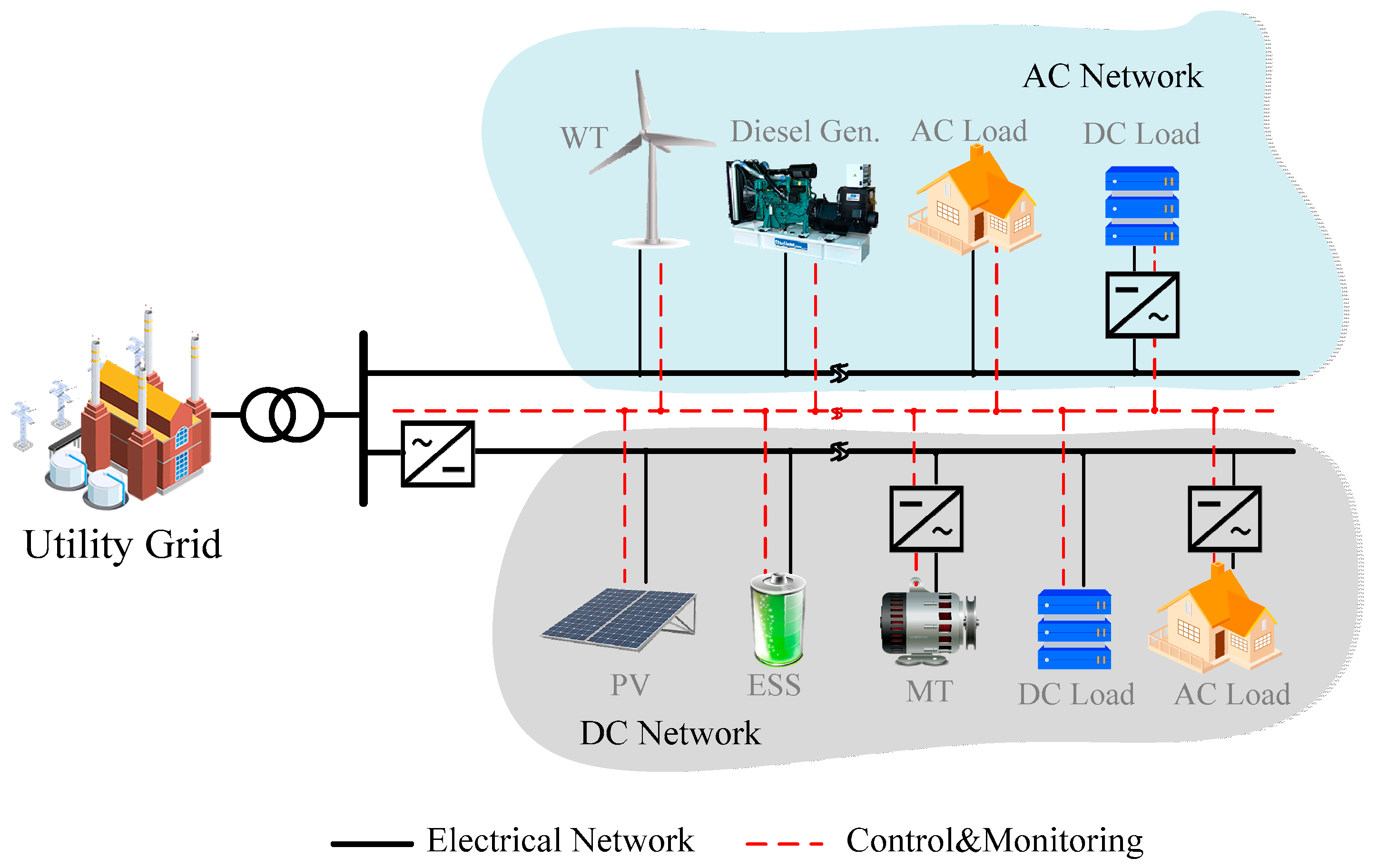
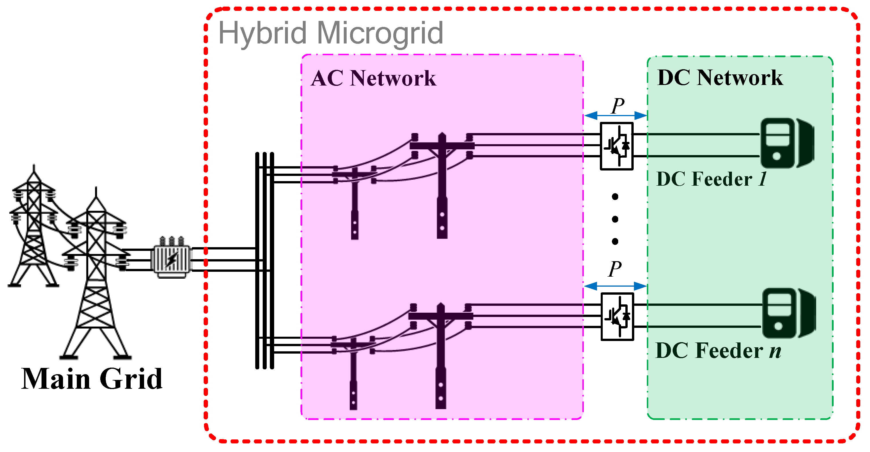
3.1. Case Study I: IEEE 33-Bus Distribution System

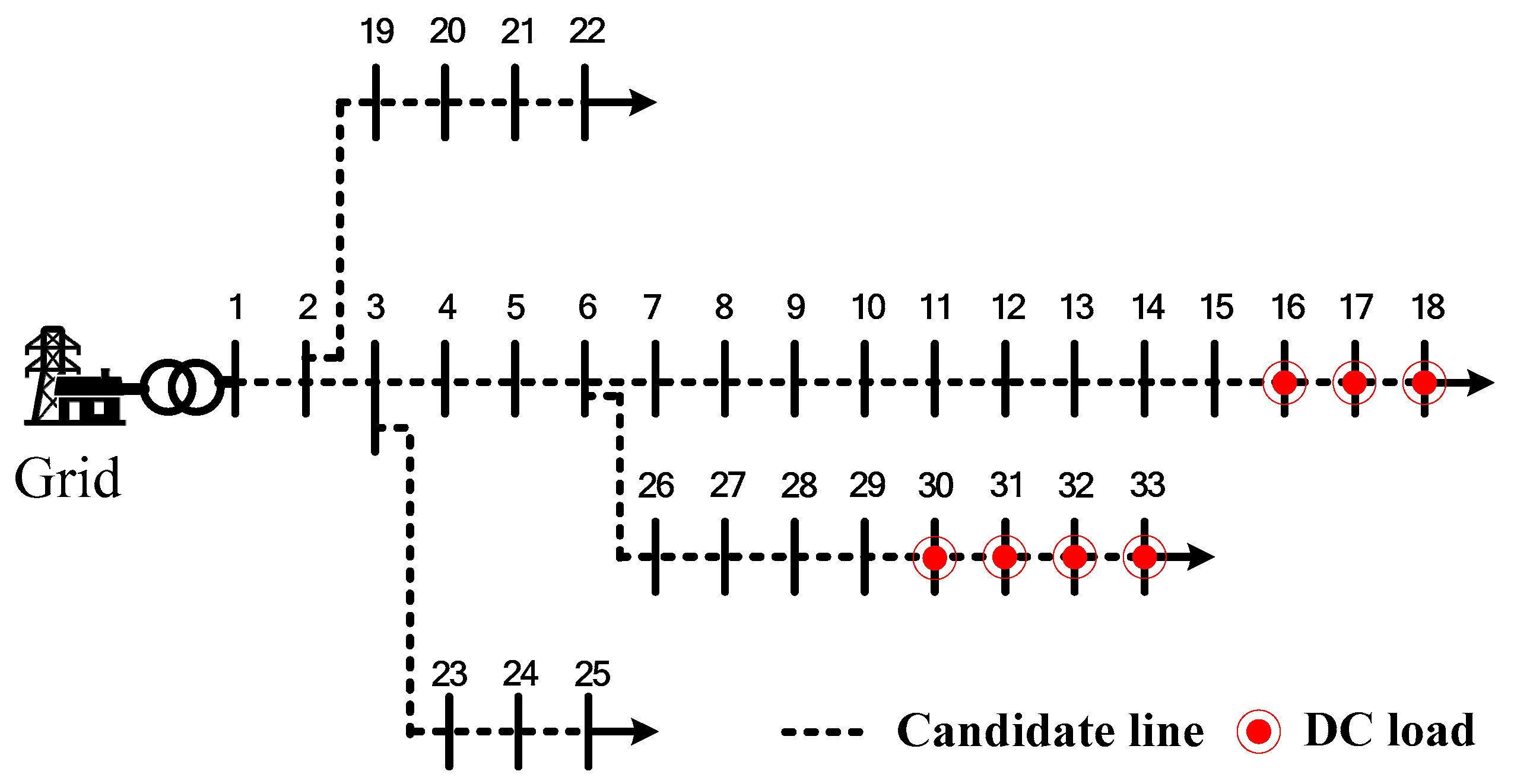
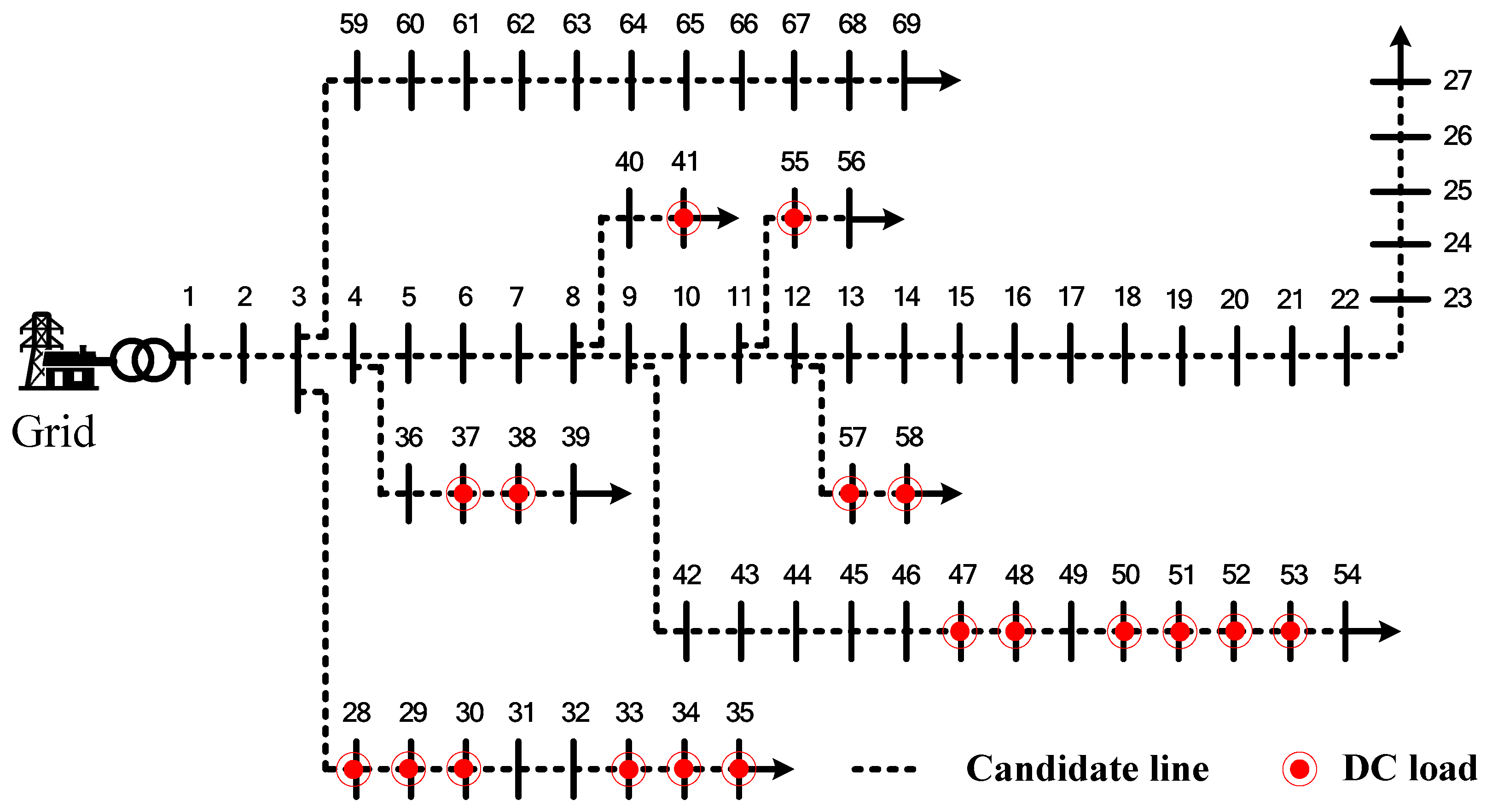
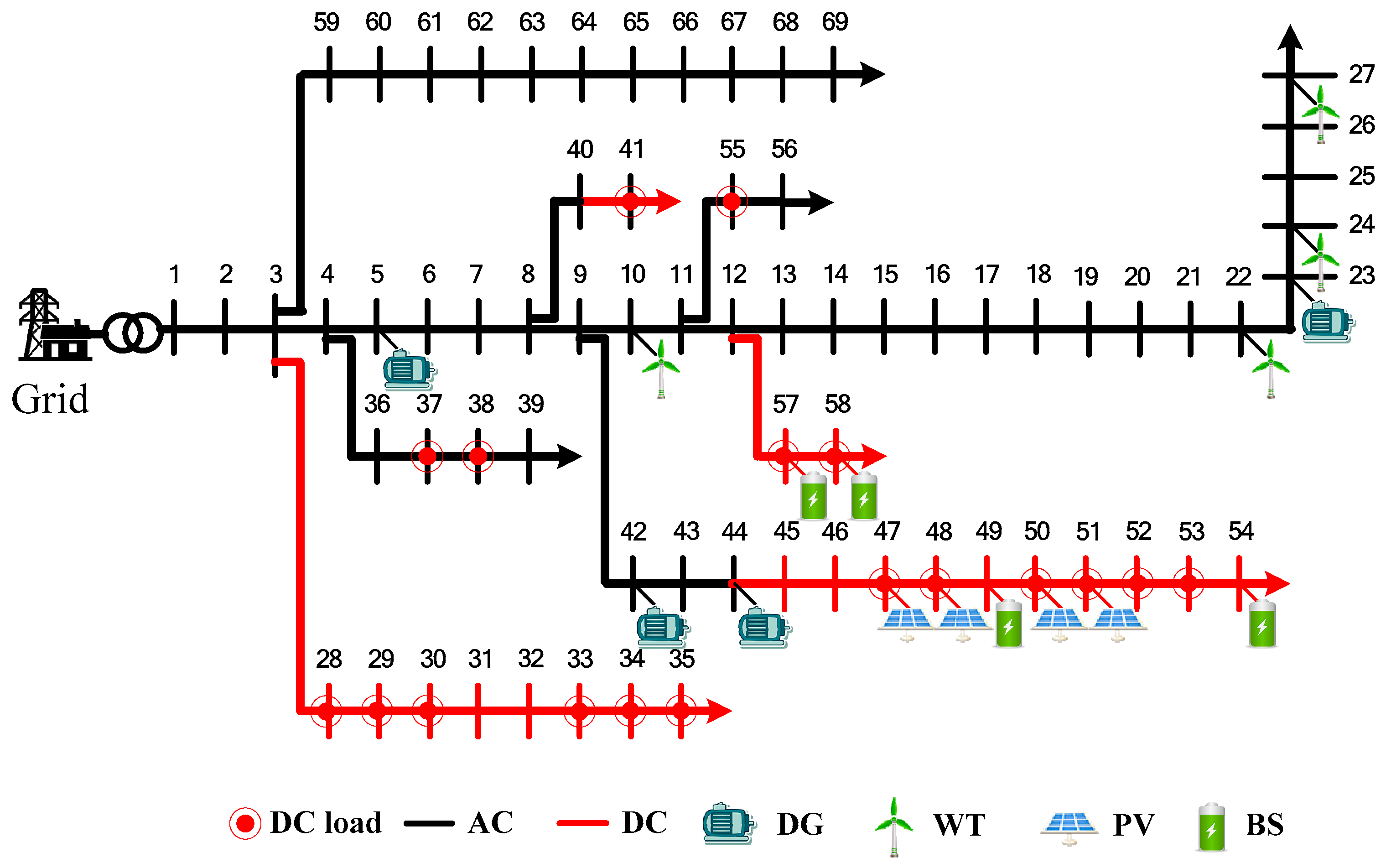
The configuration of the tested MG is shown in Figure 4, where DC loads are identified by red circles. The peak load of the MG is about 3MW. The candidate DERs include four DGs, four WTs, two PVs, and two BSs. The parameters of these DERs are shown in

Table 1. Technical Parameters of DERs.

Type	Rated Power (kW)	Investment ($/kW)	Lifespan (year)	Fuel Cost ($/kWh)	Number Limit
DG	400	300	10	0.16	4
WT	300	1200	20	0	4
PV	250	1600	20	0	2

and

Table 2. Technical Parameters of BSs.

Type	Pmax (kW)	Emax (kWh)	Power Cost ($/kW)	Energy Cost ($/kWh)	Lifespan (year)	Number Limit
BS	200	500	270	150	10	2

. The costs of investing converter and distribution lines are given in

Table 3. Investment Costs of Converters.

Converter Type	Investment ($/kW)	Lifespan (year)
AC/DC Inverter	50	15
DC/AC Inverter	60	15

and

Table 4. Investment Costs of Distribution Lines.

Type	Investment ($/m)	Lifespan (year)
AC transmission line	5	30
DC transmission line	6	30

. These data are mainly adapted from [31,32,33]. Both the charging and discharging efficiencies of BSs are set to be 0.9. In addition, the initial energy level in BSs is set to be a half of their capacity. Daily electricity prices are shown in

Table 5. Electricity Prices.

Time of Use	Off-Peak1 (23:00–07:00)	Off-Peak2 (07:00–10:00, 15:00–18:00, 21:00–23:00)	Peak1 (10:00–11:00, 13:00–15:00, 18:00–21:00)	Peak2 (11:00–13:00)
Electricity price ($/kWh)	0.057	0.126	0.198	0.216

, when the selling price is 0.8 times the buying price. The candidate buses for DER integration are shown in

Table 6. Candidate Buses for DER Integration.

DER Type	Candidate Buses
DG	5 6 7 19 23 25 29 31
BS	2 3 4 11 13 17 30
WT	9 8 10 15 18 20 22 24 27
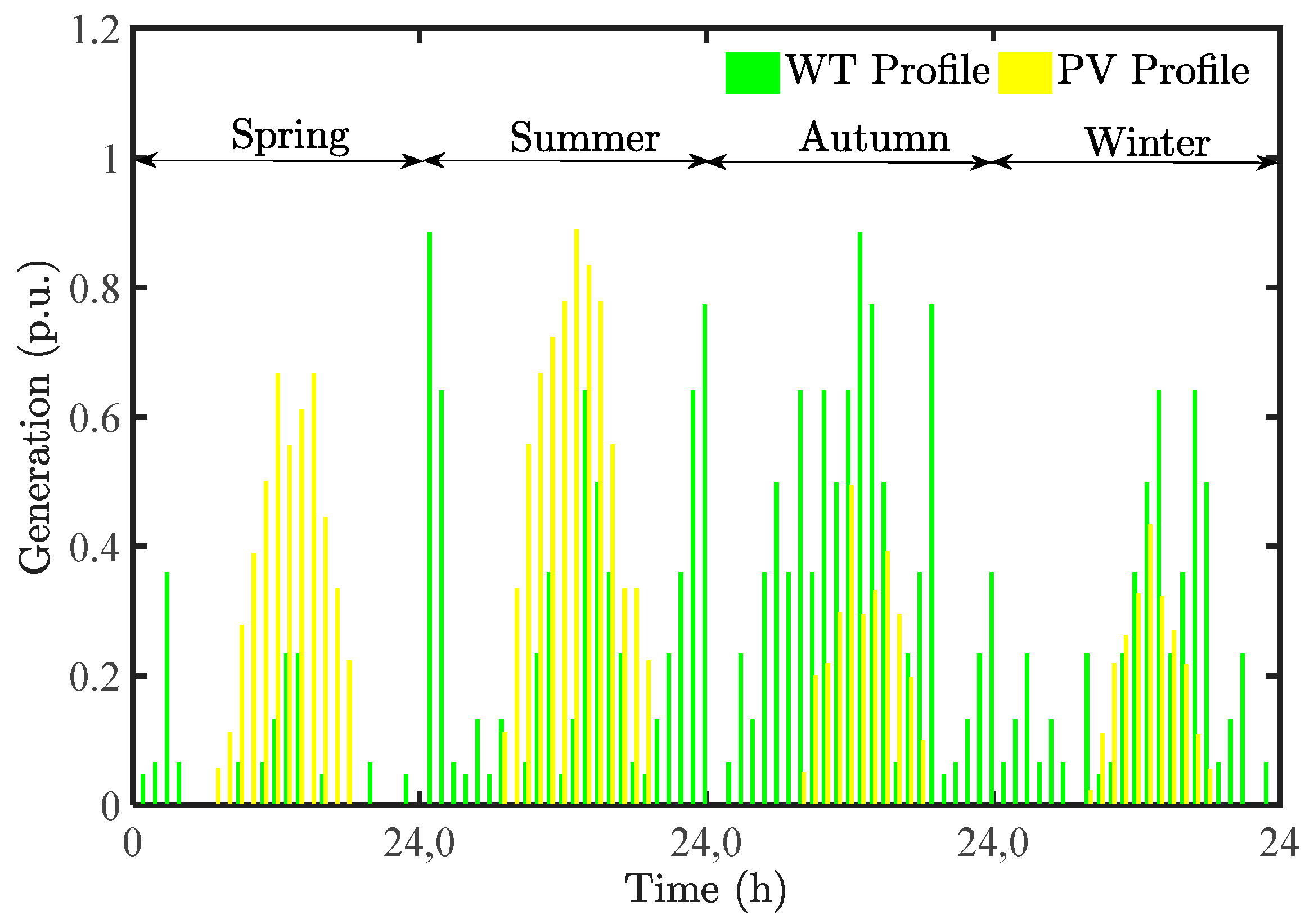
PV	12 14 16 21 26 28 32 33

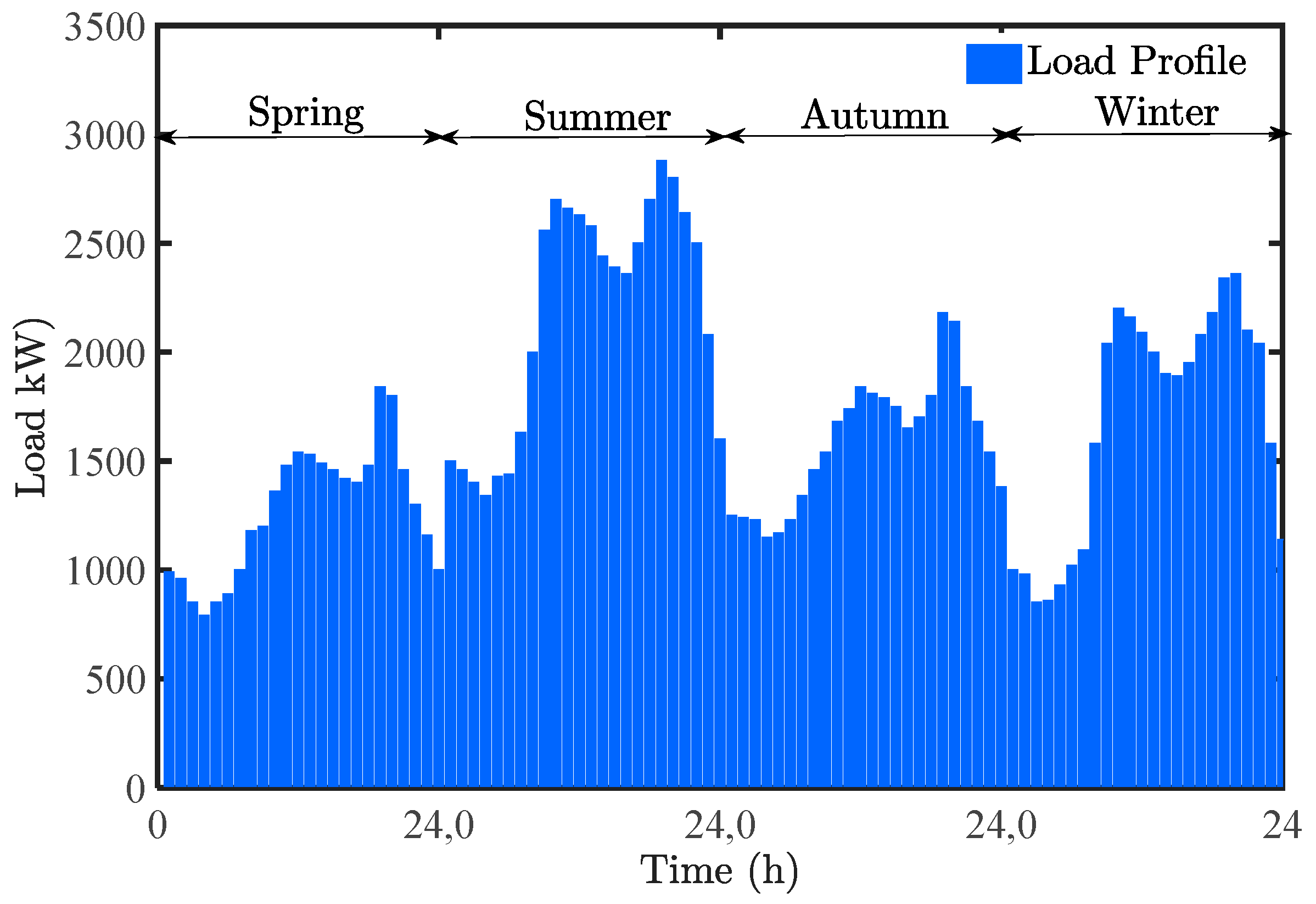
. Four typical days are selected to represent four seasons of a year. The typical generation profiles of WTs and PVs are shown in Figure 5, while the typical load profile is shown in Figure 6.

Four cases are conducted to test the effectiveness of the proposed model:

Case 1:

Hybrid AC/DC MG planning with the proposed model;

Case 2:

Hybrid AC/DC MG planning with arbitrary placement of DC feeders;

Case 3:

Pure DC MG planning;

Case 4:

Pure AC MG planning;

(1) Case Analysis: Case 1

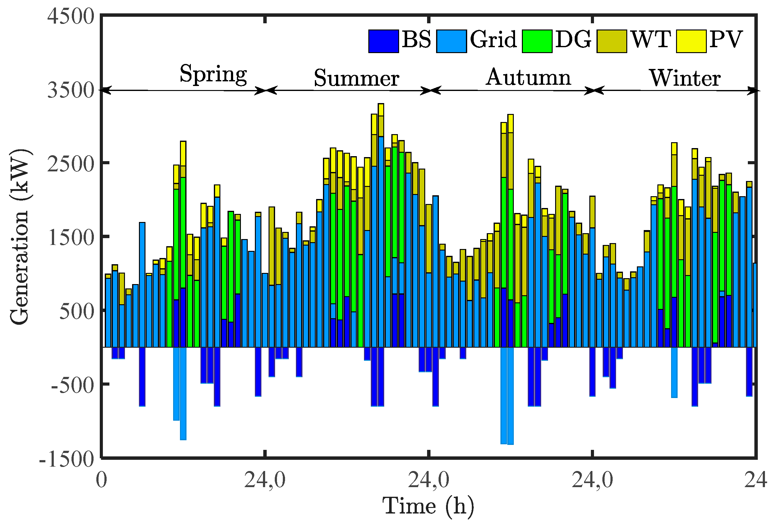
Case 1 is conducted based on the proposed model. The optimization result finds the number and placement of DERs in the MG. The annual cost and power generation of DERs are shown in

Table 7. Annual Cost and Generation of DERs in the MG.

DER	Investment Cost (103 $)	Operation Cost (103 $)	Generation Amount (MWh)	Converter Cost ($)	Average Cost ($/kWh)
DG1	23.4	217.3	1347	0	0.178
DG2	23.4	185.1	1147	0	0.182
DG3	23.4	213.3	1319	0	0.179
BS1	32.0	-	959	0	-
BS2	32.0	-	1174	0	-
WT1-WT4	39.4	0	605	0	0.065
PV1-PV2	43.8	0	390	0	0.112

. The generation schedule of DERs in the typical days is shown in Figure 7.

DERs including three DGs, two BS, four WTs and two PVs are installed for satisfying the load in the MG. Surplus power generated by renewable energy resources (such as WTs and PVs) is sold to the utility grid.

Table 7 records the detailed cost and power generation of the DERs. It can be easily seen that, the average cost of DGs is higher than that of other DERs, while the average cost of WTs and PVs is much lower than that of other DERs. Three DGs out of the four candidate DGs are installed, although the generation of DGs is not cheap. However, there are some periods (e.g., Peak 1 and Peak 2 hours) during which the local generation of DGs is more economic. In addition, these DGs shoulder the burden of serving the load when the MG is in autonomous mode in cases of faults. As to renewable energy resources, all the candidate WTs and PVs are installed in the MG. This is because the generation of WTs and PVs are cheap. Note that the average cost of WTs is less than that of PVs. On one hand, the unit investment of WTs is less than that of PVs. On the other hand, the annual energy generation amount (605 MWh) of WTs is more than that (390 MWh) of PVs. All the candidate BSs are installed, which is because the volatile electricity prices put BSs in such a favorable position that BSs can take full advantage of electricity price gap to reduce the cost. An interesting phenomenon is that the converter cost of all the DERs is zero due to the fact that all the AC based DERs are installed in the AC system while all the DC based DERs are installed in the DC feeders.

Figure 7 gives the generation schedule of DERs in the MG in the typical days of four seasons. Since the electricity price is low most of the time, the majority of power supply is purchased from the utility grid. During certain high-price periods, power generated from local DERs is even sold to the utility grid to increase the revenue. The generation of WTs and PVs is relatively cheap and therefore WTs and PVs are utilized to generate power to the fullest. The BSs take advantage of the energy price gap to make a profit during the day. As seen in Figure 7, they charge during off-Peak1/off-Peak 2 hours while discharging during Peak 1/Peak2 hours. Obviously, the schedule demonstrates the economic operation of the DERs.

(2) The Exactness of the Relaxation Technique

The proposed model relaxes the power flow equality constraint into inequality for each line. To test the computational performance of the relaxation technique, we firstly define the maximum relaxation error in the day as the relaxation gap:

$$ga{p}_{ij}=\underset{t=1,\dots ,24}{\max }\left\{(i_{ijt}^{\prime }+v_{it}^{\prime }-\Vert \begin{array}{c}2p_{ijt}\\ 2q_{ijt}\\ i_{ijt}^{\prime }-v_{it}^{\prime }\end{array}\Vert )/\Vert \begin{array}{c}2p_{ijt}\\ 2q_{ijt}\\ i_{ijt}^{\prime }-v_{it}^{\prime }\end{array}\Vert \right\}\forall (i,j)\in L$$

(83)

The relaxation gap pertinent to each distribution line in Case 1 is tested. The gap of all the lines is very small. We choose several AC and DC distribution lines to illustrate the gap in

Table 8. Relaxation Gap for Certain Distribution Lines in Case 1.

Line	Gap (10−7)	Line	Gap (10−7)	Line	Gap (10−7)
(6,7)	1.14	(10,11)	1.16	(14,15)	1.17
(7,8)	1.15	(11,12)	1.16	(15,16)	1.18
(8,9)	1.16	(12,13)	1.15	(16,17)	1.21
(9,10)	1.16	(13,14)	1.17	(17,18)	1.19

. The maximum gap is 1.21 × 10⁻⁷ which corresponds to line (16,17). Besides, the gap for DC distribution lines tends be larger than that of AC distribution lines. However, the gap is still very small, which verifies the exactness of the relaxation techniques.

(3) Comparison of the Four Cases

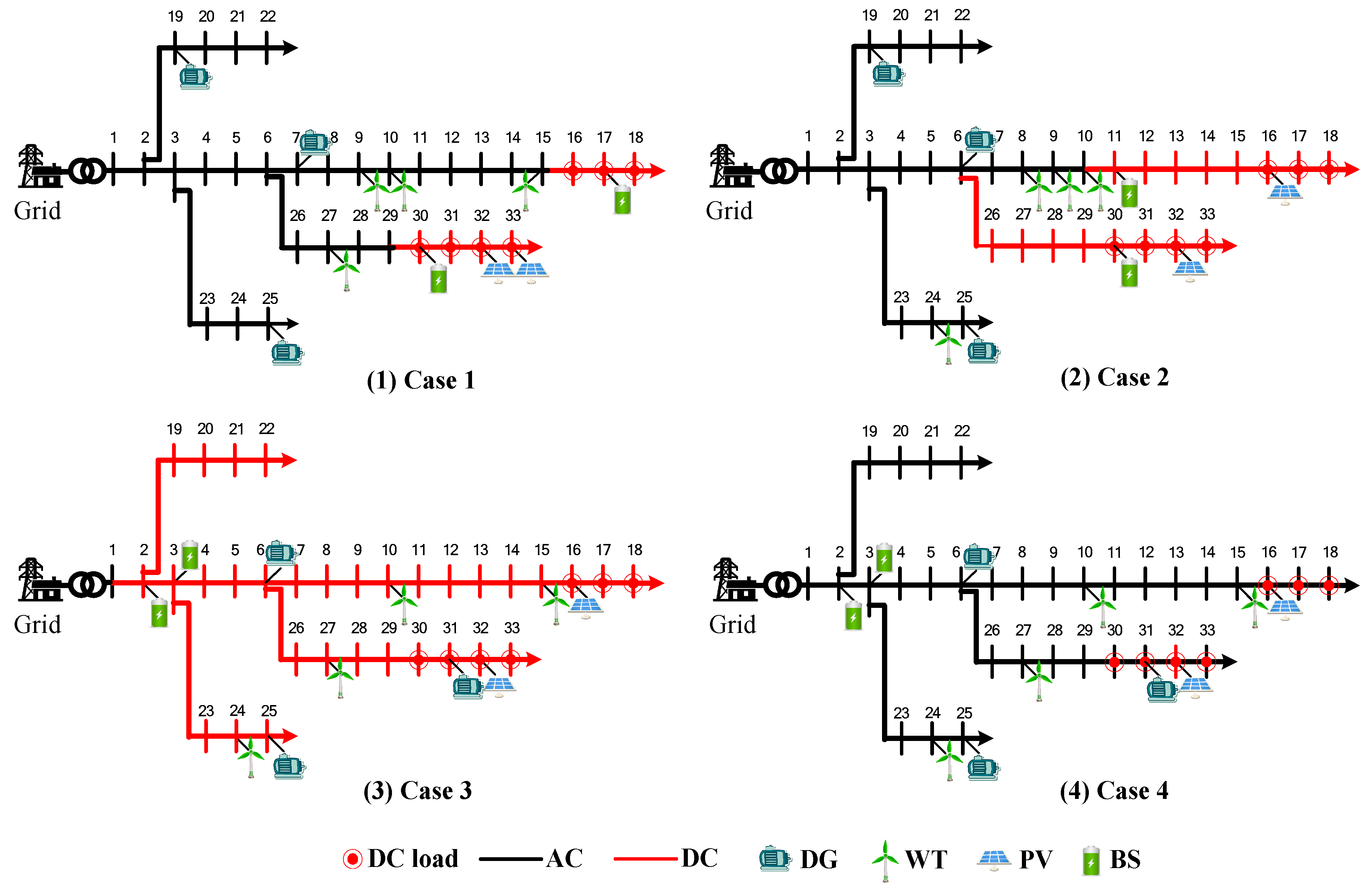
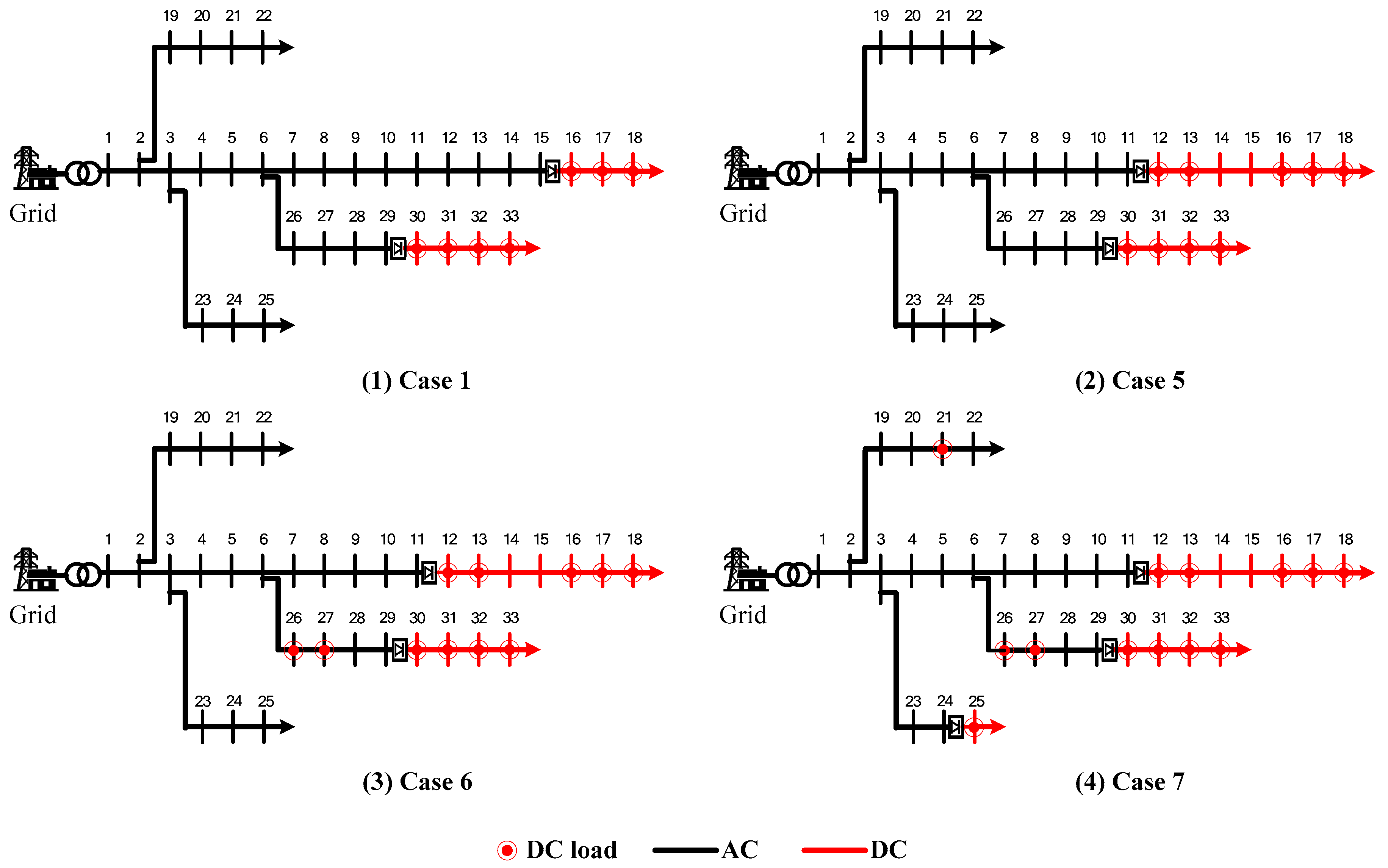
To demonstrate the advantage of the proposed model, results of all the four cases are compared. The placement of DERs and the location of DC feeders in the four cases are displayed in Figure 8, while the detailed annual investment and operation costs are listed in

Table 9. Detailed Annual Investment and Operation Costs of the Four Cases.

Case	DERs Investment (103 $)	DERs Operation (103 $)	DER Converters (103 $)	Load Converters (103 $)	Feeder Converters (103 $)	AC Lines (103 $)	DC Lines (103 $)	Total Cost (103 $)
Case 1	379.5	1383.7	0	0	4.6	46.8	14.4	1829.1
Case 2	379.5	1383.7	0	3.8	8.1	30.5	27.5	1832.7
Case 3	379.5	1383.7	16.7	14.7	18.6	0	51.9	1860.2
Case 4	379.5	1383.7	9.7	5.8	0	64.9	0	1840.0

.

As can be seen in Figure 8, two DC feeders are deployed in Case 1. All the DC loads are covered in the DC feeders while all the AC loads are covered in the AC system. Intuitively, this result is conforms to the rule of the economics, which is because the AC/DC network supplying with the same AC/DC type of loads can reduce the number of converters. Similarly, to reduce the number of converters, all the DC based DERs such as PVs and BSs are installed in the DC feeders. While all the AC based DERs such as DGs and WTs are installed in the AC system. In Case 2, two arbitrary DC feeders are formed. Note that all the DC based DERs such as BSs and PVs are installed at DC buses to save the cost of converters. This is similar to Case 1. However, the original AC loads in the DC feeders have to use converters, leading to an additional investment cost. The detailed cost is listed in Table 9. In Case 3, all the branches and buses are DC based. The DERs are distributed randomly in the network. Any positions make no difference for DERs in this case as long as the network security is guaranteed. In Case 4, all the branches and buses are AC based. This is a conventional AC MG planning problem. The analysis of this case is similar to that of Case 3 and not repeated here.

From Table 9, the investment and operation costs in the four cases are the same. As we know, the total loads in the MG are the same in the four cases. In fact, from the perspective of energy balance, the capacity of the installed DERs in Case 1 is completely the same as that in Case 2 and Case 4. Therefore, the investment and operation costs in four cases are the same. The total cost in Case 3 is the most among the four cases. This is because most of the loads are AC loads, while the MG is a DC MG. Therefore a lot of converters are needed for AC loads. As can be seen in Table 9, the load converter cost and feeder converter cost in Case 3 are much higher than those in other cases. It should be noted that DC feeders need only two distribution lines while AC feeders need three distribution lines. The investment cost of distribution lines in Case 3 is the least. Although the DC MG saves a lot in distribution line investment, the saved cost still can’t offset the cost brought by the converters. The total cost in Case 1 is the least among the four cases. This is mainly because the cost of load converters and feeder converters is much less. The DC feeders cover the least AC loads and save a lot of unnecessary converters. From the analysis above, we can conclude that the planning problem is essentially to find an optimal balance between the investment of distribution lines and converters.

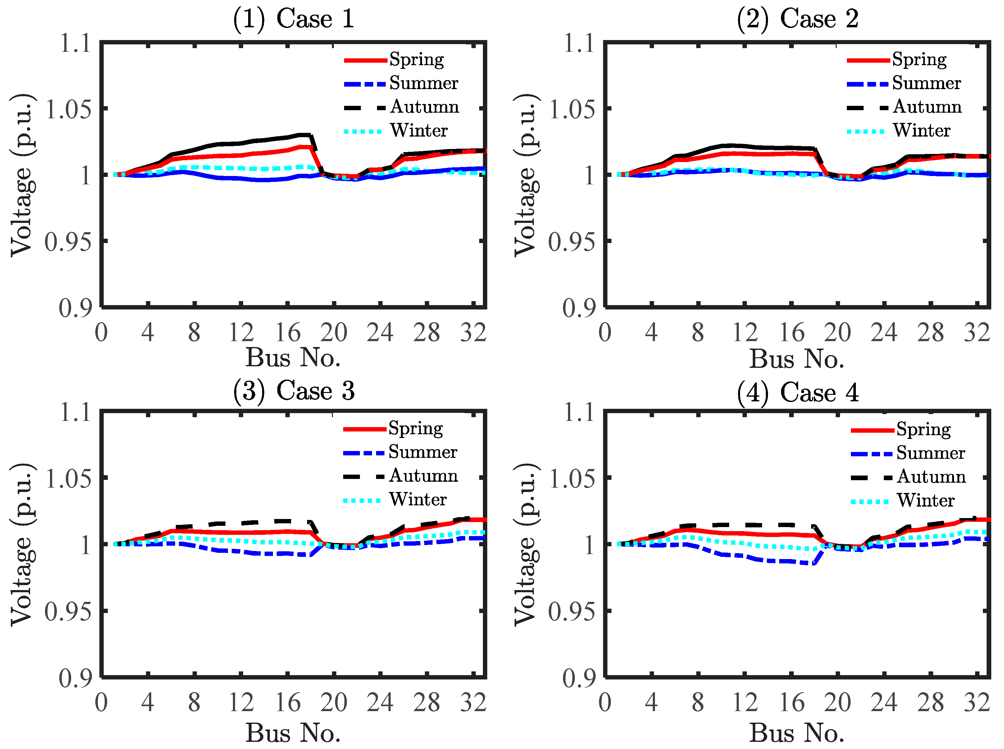
The voltage of the buses at 12:00 when the load level is relatively high in the typical days is shown in Figure 9. As can be seen, all the voltage is between the safe intervals [0.9, 1.1]. There are some voltage fluctuations between the nodes. This is partly due to the placement of DERs and partly due to the network configuration. Taking bus 17 in Case 1 as an example, the voltage rises rapidly there because of the placement of BSs, which support the voltage by generating power.

Note that the voltage level is higher at bus 17 than that at the root bus 1. This is because the electricity price is high at that time. Many DERs such as DGs and BSs are started up to generate power and sell it to the grid utility to increase the revenue. So the power flow is reversed and flows from the end bus to the root bus. Therefore the voltage is elevated a lot at the end buses. It is interesting to find that the voltage in Case 3 is similar to that of Case 4. This is due to the fact that the placement of DERs in the DC MG and AC MG is the same, as can be seen in Figure 8. Therefore the voltage support from the DGs is similar. Anyway, the hybrid MG can operate safely in all the situations.

(4) Influence of the Distribution of DC loads

From the analysis of Case 1 to Case 4, we find that if the DC loads lie nearby, then the DC feeders are easily formed to connect those loads in the same network. To further investigate the influence of the distribution of DC loads to the formation of DC feeders, additional cases are carried out. We gradually expand the distribution of the DC loads in Case 5–Case 7. The final placement of DC feeders in each case is show in Figure 10. In Case 5, two additional loads at bus 12 and 13 are set as DC loads. In this case, the DC feeder starts from bus 11 to connect all the DC loads. This measure not only saves the cost of separate converters for DC loads, but also reduces the investment cost for distribution lines. In Case 6, we further add two DC loads at bus 26 and 27. It’s interesting to find that the two buses are not incorporated into the corresponding DC feeder. This is because the original AC bus 28 and 29 will be integrated into the DC feeder if bus 26 and 27 are incorporated into the DC feeder owing to the continuity of DC feeders. Therefore, additional AC/DC converter fee for AC loads will be charged if the two buses are included in the DC feeder. The increased cost from the AC/DC converters of bus 28 and 29 may exceed the saved cost from converters and distribution lines of the DC feeders. Therefore, the investors would prefer to supply these two DC loads through AC/DC converters in the AC system rather than expanding the DC feeder. We further scatter two DC loads at bus 21 and bus 25, respectively. It is found that bus 25 with the DC load at the terminal of the feeder is set as DC bus while bus 21 is not. This is because the investment cost of distribution lines can be reduced if the bus with DC loads at the terminal of the feeder turns to a DC bus. However, if the bus with DC loads locates at the inner part of the feeder, it’s not necessarily economic to turn to a DC bus.

Above all, the proposed model results in the optimal placement of DC feeders which achieves the tradeoff between the cost charged from AC/DC converters of AC loads and the cost saved from DC/AC converters of DC loads and DC distribution lines. Hence, we can conclude that the proposed method can determine the number and site of DERs in an economic manner. In addition, it can locate the DC feeders of the MG considering the connectivity of DC loads based on their distribution. If there are more DC loads in the network, a longer DC feeder may be more economic. However, if the DC loads are scattered in the network, it would be a more economical way to supply DC loads by deploying a partial set of DC feeders or even no DC feeders.

(5) Comparison of the Performances of the MISOCP and MILP Models

The performances of the proposed MISOCP and MILP models are compared. Since the MISOCP model involves no approximations and it is considered more accurate than the MILP model. In spite of its accuracy, the MISOCP model is time-consuming and the computation consumption reaches up to 370 min. Although the MILP model sacrifices the accuracy of the solution, it can greatly improve the computational efficiency.

As can be seen in

Table 10. Comparison of the Performances of the MISOCP and MILP Models.

Model	$\mathcal{M}$	Investment (103 $)	Operation (103 $)	Total Cost (103 $)	Time (min)
MILP	3	445.5	1367.6	1813.1	1
	4	445.5	1367.6	1813.1	1.5
	5	445.5	1370.1	1815.6	4
	6	445.5	1374.8	1820.3	58
	7	445.5	1378.8	1824.3	187
MISOCP	-	445.5	1383.7	1829.1	370

, the investment cost of the MILP model is completely the same as that of the MISOCP model, and only the operation cost makes difference due to the approximation of power flow. However, the error of the total cost is within 1% if the MISOCP model is used as a benchmark. The total cost tends to be more accurate as $\mathcal{M}$ increases. However, the computation time also grows dramatically when $\mathcal{M}$ exceeds 6. Therefore, the MISOCP model is preferred if the scale of the MG is small, otherwise the MILP model with a proper parameter $\mathcal{M}$ is better.

3.2. Case Study II: IEEE 69-Bus Distribution System

To further validate the proposed model, the IEEE 69-bus distribution system as shown in Figure 11 is also studied for planning a hybrid AC/DC MG. The parameters of candidate DERs are shown in

Table 11. Technical Parameters of DERs.

Type	Rated Power (kW)	Investment ($/kW)	Lifespan (year)	Fuel Cost ($/kWh)	Number Limit
DG	400	300	10	0.16	6
WT	200	1200	20	0	4
PV	250	1600	20	0	4

and

Table 12. Technical Parameters of BSs.

Type	Pmax (kW)	Emax (kWh)	Power Cost ($/kW)	Energy Cost ($/kWh)	Lifespan (year)	Number Limit
BS	200	500	270	150	15	4

. The candidate buses for DER integration are shown in

Table 13. Candidate Buses for DER Integration.

DER Type	Candidate Buses
DG	5 6 7 23 25 29 31 42 44 46 60 62
BS	2 30 34 38 39 41 49 54 55 56 57 58
WT	8 9 10 18 20 22 24 27 59 61 63 65
PV	12 14 16 28 32 33 35 36 47 48 50 51

. The other parameters such as the electricity price and loading level are the same as those in Case Study I. The MILP model is employed here.

According to the optimization result, four DGs, four BSs, four WTs and four PVs are installed in the MG. Figure 12 shows the placement of DERs. All the candidate renewable energy resources and BSs are installed as expected. Several candidate DGs are installed to coordinate with other DERs to satisfy the loads. In addition, all the DC based DERs such as PVs and BSs are installed at the DC buses; while all the AC based DERs such as DGs and WTs are installed in the AC system. Such a result can be analyzed similar to those in Case study I. As can be seen in Figure 12, each DC feeder only covers the nearest DC loads, while AC loads are avoided being covered due to the high expense of converters. It should be noted that buses 45, 46 are set to DC buses. This is because the reduced investment cost of DC distribution lines covers the increased investment cost of converters. The buses with the DC loads at the terminal of the feeders are all set to DC bus and incorporated into the DC feeders, while the buses with DC loads at the inner part of the feeders are not necessarily incorporated into the DC feeders. Hence, we can conclude that the model can always effectively locate the DC feeders according to the distribution of DC loads at a least cost. Therefore, all the two case studies verify the effectiveness of the proposed model.

4. Conclusions

In this paper, a hybrid AC/DC MG planning model is proposed for addressing the concerns of optimal placement of DC feeders based on the distribution of DC loads. The proposed model is comprehensive and practical, due to the consideration of hybrid AC/DC power flow equations and the continuality requirement of DC feeders. As demonstrated by case studies, the proposed model can not only select and deploy the DERs economically but also place the DC feeders in an optimal manner. The case study results justify the following conclusions: (1) It is more economic to install AC- or DC-based DERs in the power network with the same AC/DC type because of the reduction in the investment cost of converters. (2) The optimal placement of DC feeders should strikes a balance between the increased cost of investing AC lines and AC/DC converters for AC loads and the saved cost of investing DC lines and DC/AC converters for DC loads. (3) The buses with DC loads at the terminal of the feeders are all set to DC buses and integrated into the DC feeders, while those intermediate buses with DC loads are not necessarily integrated into the DC feeders. Overall, the proposed model successfully places the DC feeders for supplying the DC loads to the greatest extent while maintaining the least cost of investing converters and lines.

References

1. Nehrir, H.; Wang, C.; Strunz, K.; Aki, H.; Bing, J.; Salameh, Z. A review of hybrid renewable/alternative energy systems for electric power generation: Configurations, control and applications. IEEE Trans. Sustain. Energ. 2012, 2, 392–403. [Google Scholar] [CrossRef]
2. Nwulu, N.I.; Xia, X. Optimal dispatch for a microgrid incorporating renewables and demand response. Renew. Energ. 2017, 101, 16–28. [Google Scholar] [CrossRef]
3. Wang, M.H.; Tan, S.C.; Lee, C.K.; Hui, S.Y.R. A Configuration of Storage System for DC Microgrids. IEEE Trans. Power Electron. 2018, 33, 3722–3733. [Google Scholar] [CrossRef] [Green Version]
4. Nasir, M.; Iqbal, S.; Khan, H.A. Optimal Planning and Design of Low-Voltage Low-Power Solar DC Microgrids. IEEE Trans. Power Syst. 2018, 33, 2919–2928. [Google Scholar] [CrossRef]
5. Kaur, R.; Krishnasamy, V.; Kandasamy, N.K. Optimal sizing of wind–PV-based DC microgrid for telecom power supply in remote areas. IET Renew. Power Gener. 2018, 12, 859–866. [Google Scholar] [CrossRef]
6. Shadmand, M.B.; Balog, R.S. Multi-Objective Optimization and Design of Photovoltaic-Wind Hybrid System for Community Smart DC Microgrid. IEEE Trans. Smart Grid 2014, 5, 2635–2643. [Google Scholar] [CrossRef]
7. Hong, T.; Leon, F.D. Centralized Unbalanced Dispatch of Smart Distribution dc Microgrid Systems. IEEE Trans. Smart Grid 2018, 9, 2852–2861. [Google Scholar] [CrossRef]
8. Xiao, J.; Wang, P.; Setyawan, L.; Xu, Q. Multi-Level Energy Management System for Real-Time Scheduling of DC Microgrids With Multiple Slack Terminals. IEEE Trans. Energy Convers. 2016, 31, 1–9. [Google Scholar] [CrossRef]
9. Phurailatpam, C.; Rajpurohit, B.S.; Wang, L. Planning and optimization of autonomous DC microgrids for rural and urban applications in India. Renew. Sustain. Energy Rev. 2018, 82, 194–204. [Google Scholar] [CrossRef]
10. Nutkani, I.U.; Meegahapola, L.; Andrew, L.P.C.; Blaabjerg, F.; Royal Melbourne Institute of Technology (RMIT); The Chinese University of Hong Kong; Aalborg University. Autonomous power management for interlinked AC-DC microgrids. CSEE J. Power Energy Syst. 2018, 4, 11–18. [Google Scholar] [CrossRef]
11. Baboli, P.T.; Shahparasti, M.; Mohamadian, M.; Moghaddam, M.P.; Haghifam, M.R. Energy management and operation modelling of hybrid AC–DC microgrid. IET Gener. Transm. Distrib. 2014, 8, 1700–1711. [Google Scholar] [CrossRef]
12. Papari, B.; Edrington, C.S.; Bhattacharya, I.; Radman, G. Effective Energy Management of Hybrid AC-DC Microgrids with Storage Devices. IEEE Trans. Smart Grid 2017, 10, 193–203. [Google Scholar] [CrossRef]
13. Zhao, B.; Qiu, H.; Qin, R.; Zhang, X.; Gu, W.; Wang, C.; Haifeng, Q.; Xue-Song, Z. Robust Optimal Dispatch of AC/DC Hybrid Microgrids Considering Generation and Load Uncertainties and Energy Storage Loss. IEEE Trans. Power Syst. 2018, 33, 5945–5957. [Google Scholar] [CrossRef]
14. Lotfi, H.; Khodaei, A. AC Versus DC Microgrid Planning. IEEE Trans. Smart Grid 2017, 8, 296–304. [Google Scholar] [CrossRef]
15. Lotfi, H.; Khodaei, A. Hybrid AC/DC microgrid planning. Energy 2017, 118, 37–46. [Google Scholar] [CrossRef]
16. Ahmed, H.M.; Eltantawy, A.B.; Salama, M.M. A planning approach for the network configuration of AC-DC hybrid distribution systems. IEEE Trans. Smart Grid 2018, 9, 2203–2213. [Google Scholar] [CrossRef]
17. Garces, A. On the Convergence of Newton’s Method in Power Flow Studies for DC Microgrids. IEEE Trans. Power Syst. 2018, 33, 5770–5777. [Google Scholar] [CrossRef]
18. Li, J.; Liu, F.; Wang, Z.; Low, S.H.; Mei, S. Optimal Power Flow in Stand-alone DC Microgrids. IEEE Trans. Power Syst. 2018, 33, 5496–5506. [Google Scholar] [CrossRef]
19. Li, C.; Chaudhary, S.K.; Savaghebi, M.; Vasquez, J.C.; Guerrero, J.M. Power flow analysis for low-voltage AC and DC microgrids considering droop control and virtual impedance. IEEE Trans. Smart Grid 2017, 8, 2754–2764. [Google Scholar] [CrossRef]
20. Therrien, F.; Jatskevich, J.; Wong, V.W.; Bahrami, S. Semidefinite Relaxation of Optimal Power Flow for AC-DC Grids. IEEE Trans. Power Syst. 2017, 32, 289–304. [Google Scholar]
21. Ding, T.; Li, C.; Yang, Y.; Blaabjerg, F.; Zhang, Y.; Yan, H. Second-order cone programming relaxation-based optimal power flow with hybrid VSC-HVDC transmission and active distribution networks. IET Gener. Transm. Distrib. 2017, 11, 3665–3674. [Google Scholar] [CrossRef]
22. Elsayed, A.T.; Mohamed, A.A.; Mohammed, O.A. DC microgrids and distribution systems: An overview. Electr Power Syst. Res. 2015, 119, 407–417. [Google Scholar] [CrossRef]
23. Ding, T.; Lin, Y.; Bie, Z.; Chen, C. A resilient microgrid formation strategy for load restoration considering master-slave distributed generators and topology reconfiguration. Appl. Energy 2017, 199, 205–216. [Google Scholar] [CrossRef]
24. Wang, Z.; Chen, B.; Wang, J.; Kim, J.; Begovic, M.M. Robust Optimization Based Optimal DG Placement in Microgrids. IEEE Trans. Smart Grid 2014, 5, 2173–2182. [Google Scholar] [CrossRef]
25. Ding, T.; Lin, Y.; Li, G.; Bie, Z. A New Model for Resilient Distribution Systems by Microgrids Formation. IEEE Trans. Power Syst. 2017, 32, 4145–4147. [Google Scholar] [CrossRef]
26. McCormick, G.P. Computability of global solutions to factorable nonconvex programs: Part I—Convex underestimating problems. Math. Program. 1976, 10, 147–175. [Google Scholar] [CrossRef]
27. Farivar, M.; Low, S.H. Branch Flow Model: Relaxations and Convexification—Part I. IEEE Trans. Power Syst. 2013, 28, 2554–2564. [Google Scholar] [CrossRef]
28. Ben-Tal, A.; Nemirovski, A. On Polyhedral Approximations of the Second-Order Cone. Math. Oper. 2001, 26, 193–205. [Google Scholar] [CrossRef]
29. Baran, M.E.; Wu, F.F. Network reconfiguration in distribution systems for loss reduction and load balancing. IEEE Trans. Power Deliv. 1989, 4, 1401–1407. [Google Scholar] [CrossRef]
30. Naik, S.N.G.; Khatod, D.K.; Sharma, M.P. Analytical approach for optimal siting and sizing of distributed generation in radial distribution networks. IET Gener. Transmi. Distrib. 2014, 9, 209–220. [Google Scholar] [CrossRef]
31. Zou, K.; Agalgaonkar, A.P.; Muttaqi, K.M.; Perera, S. Distribution System Planning With Incorporating DG Reactive Capability and System Uncertainties. IEEE Trans. Sustain. Energy 2012, 3, 112–123. [Google Scholar] [CrossRef]
32. Zhang, J.; Cheng, H.; Wang, C. Technical and economic impacts of active management on distribution network. Int. J. Electr. Power Energy Syst. 2009, 31, 130–138. [Google Scholar] [CrossRef]
33. Cao, X.; Wang, J.; Zeng, B. A Chance Constrained Information-Gap Decision Model for Multi-Period Microgrid Planning. IEEE Trans. Power Syst. 2018, 33, 2684–2695. [Google Scholar] [CrossRef] [Green Version]
Figure 1. Configuration of a typical hybrid AC/DC MG.
Energies 12 01751 g001
Figure 2. The proposed planning framework of the hybrid MGs.
Energies 12 01751 g002
Figure 3. Illustration of the continuity of the DC feeders.
Energies 12 01751 g003
Figure 4. Structure of the IEEE 33-bus distribution system based MG.
Energies 12 01751 g004
Figure 5. Typical generation profiles of WTs and PVs in four seasons.
Energies 12 01751 g005
Figure 6. Typical load profile in four seasons.
Energies 12 01751 g006
Figure 7. The generation schedule of DERs in the MG in the typical days.
Energies 12 01751 g007
Figure 8. Placement of DERs in the four cases.
Energies 12 01751 g008
Figure 9. Voltage of Buses in the four cases in typical days.
Energies 12 01751 g009
Figure 10. Influence of the distribution of DC loads on the formation of DC feeders.
Energies 12 01751 g010
Figure 11. Structure of the IEEE 69-bus distribution system based MG.
Energies 12 01751 g011
Figure 12. Placement of DERs in the MG in Case Study II.
Energies 12 01751 g012