A Demand Response Approach to Scheduling Constrained Load Shifting

Abstract

Demand response (DR) and its advantages are nowadays unquestionable due to the success of several recent implementations of DR programs. Improved methodologies and approaches are needed for the adequate consumers’ schedule in DR events, taking the consumers’ behaviour and preferences into account. In this paper, a virtual power player manages DR programs, minimizing operation costs, respecting the consumption shifting constraints. The impact of the consumption shifting in the target periods is taken into consideration. The advantages of the DR use in comparison with distributed generation (DG) are evaluated. Two scenarios based on 218 consumers in a frame of 96 periods have been implemented. It is demonstrated the advantages of DR in the operation of distributed energy resources, namely when considering the lack of supply.

1. Introduction

The definition of demand response includes the changes in the consumption in response to variations in the electricity price, or to incentives applied in cases of high market prices or when the system reliability needs improvement [1]. More recent definitions, namely at the European level, divide DR programs into implicit and explicit DR [2].

The current real market and power system integration of DR programs’ state makes possible to find several successful implementations [3,4]. It is necessary to consider all the resources providing demand response, including the small size ones in order to catch the full potential and competitiveness of flexible loads [5,6,7]. Regulatory documents have pointed out to enforce the opportunities for demand response, the same as generation. For instance, in FERC Order No. 719 [8]. In the case of Europe, some changes are noticed [2,9].

Virtual power players (VPPs) appeared in the new context of power systems operation, aggregating small size resources. Distinct classifications are given according to the types of resources [10]. In fact, a VPP can aggregate demand response and distributed generation (DG) resources, and manage the distribution network [6,11].

The present paper addresses the economic advantages and the effectiveness of DR. The paper includes a sensitivity analysis on the impact of the DR prices for the VPP operation costs and the cost comparison of DG and DR when facing supply unavailability. The advantages of using DR as an alternative to DG in such situation are analyzed, discussed, and illustrated using real data.

Section 2 provides the discussion of the related work and the contribution of the paper. Section 3 includes the DR model. Section 4 includes the optimization model. Section 5 includes the case study, and Section 6 the results. Section 7 presents the main conclusions of the work.

2. Related Work and Contribution

In the literature, it is possible to find several works that refer to the need of providing adequate attention to consumers’ flexibility for the implementation of DR programs. Focusing on consumption devices and energy management appliances, in [12] some benefits are explored. Regarding the network itself, in [13] the load shifting influence in reliability indices is discussed, where load shifting is applied to seven types of load. In [14], the contribution of DR to reliability concerns considering the uncertainty of the consumer’s response is discussed.

It is also important to refer to the issue of communications in the context of DR programs implementation. The work presented in [15] addresses the large-scale direct load control implementation, namely considering communication issues.

For a more complete discussion on the integration of DR resources, in [16] it is presented an approach that considers electric water heaters used in the scope of balancing wind generation. Focusing on thermal storage, the work in [17] presents a stochastic approach for DR implementation.

The authors of [18] proposed a methodology for the optimal scheduling of DR, providing constraints to the load shifting and curtailment, maximizing the aggregator profits. The DR contracts are established between the independent system operator (ISO) and the aggregators. In [19], the use of DR in order to improve the integration of wind and PV on roof-tops is addressed. The work in [20] is focused on retailers, dealing with the profitability of such players when electricity market prices rise by adequately defining the incentives to be paid to consumers in DR programs. These works are mostly focusing on the way that different players use DR in order to achieve their goals in market participation or in buildings energy management.

With deep concern about virtual power plants, scheduling optimization considering DR is presented in [21,22,23]. In [21,22], the DR uncertainty is addressed by using stochastic approaches for the maximization of virtual power plant profit. Different DG resources are included. In [23], the scheduling of thermal energy resources is made together with the scheduling of electrical energy resources.

The works mentioned above refer to the DR potential, lacking the modeling of consumers. In fact, in [24] the authors have introduced the model of the consumption shifting in the context of distributed energy resource scheduling.

In the present paper, the proposed method contributes to the definition of preferences by the consumers regarding the shifting of loads between periods. Such preferences are modeled as constraints of the optimization developed for the optimal scheduling of resources by a VPP aggregating DR and DG. The main contributions can be seen from the past literature concerning VPPs, namely from the authors’ past works as presented in [25,26] regarding the number of periods in which DR events are applied. In fact, in [25,26], the authors propose the use of DR, in the scope of a VPP, for several operation scenarios but always considering the optimization of the resources in a single period. The load is curtailed and reduced but never shifted to distinct periods. In what concerns the scientific works from other authors, in the scope of a VPP or not, we can find a major contribution of the present work on the consumers’ possibility to implement load shifting preferences.

The work in [27] presents an updated VPP operation model including DR, where the load shifting modeling is presented in a simpler way than in the present work. In [28] a methodology for the bidding of load shifting is presented, focusing on the number of bids and of sub-loads. A deep analysis of the bidding issues is presented considering the available amount of shiftable load. However, the present work provides contribution to the consumption shifting constraining (modeling limits for each period/set of periods) from the VPP and the consumer standpoints.

Summarizing, the contributions in the present paper are the following:

• Addressing the economic advantages and effectiveness of DR
• Providing a sensitivity analysis on the impact of the DR prices for the VPP operation costs
• Comparing the cost of DG and DR when facing supply unavailability
• Showing the advantages of using DR as an alternative to DG, using real data scenario
• Addressing the remuneration of each consumption cluster.

3. Demand Response Approach

The proposed DR approach is driven to integrate the schedule of demand response and supply sources, managed by a Virtual Power Player (VPP). Figure 1 depicts the resources aggregation by the VPP. As in Figure 1, the model includes the following assumptions:

• The VPP can use supply resources that are limited in the maximum supply power in each period. Supply resources are available to the VPP in the electrical connections of the managed distribution network with the upstream network. It is also considered the existence of several DG types;
• Using such resources, the VPP ensures the adequate remuneration of distributed generation and demand response actual contribution;
• As to the consumers, the VPP manages their flexibility in several consumption clusters (ct), ct1 to CtN. Numerous constraints are applied to the consumption shifting described in Section 3;
• The VPP resources scheduling is performed for each period respecting the respective remuneration, minimizing the total operation costs for the overall scheduling horizon.

In the case of ct1, presented in Figure 1, the VPP can shift part of the load from period 3 to period 4. For a generic cluster CtN, seen in the bottom of Figure 1, the critical periods are seen in Figure 2, regarding the load changes influencing period t. As can be seen, it is possible to shift load from period t to periods before and after period t. Consumption reduction is also illustrated. Considering the load shifting (in or out) and the load reduction, the final load is lower than the initially expected. The terms “DR shift in” and “DR shift out” represent the consumption that is moved from one period (out) to another period (in). For example, the consumption of a washing machine can be moved from a period (DR shift out) to another period (DR shift in). The term “rigid demand” refers to the consumption that is kept in each period (i.e. the initial demand minus the reduced and shifted load).

The details of the timeline concerning the consumption shifting process are in Figure 2. In the proposed DR model, the VPP performs the resource’s schedule for T, considering the DR events to be declared during that period. Figure 2 shows one DR event in the scheduling horizon. The user is able to specify backward and forward shifting periods.

The load shifting parameters include the limit of power shifted and the respective remuneration. Several constraints are considered related with the limit load shifting, for each ct. It also takes into consideration the energy supply and DG remuneration and technical limits. These constraints address the consumers and VPP’s concerns and goals.

The proposed methodology is built on the assumption that the scheduled consumption shifting is ensured by the consumers either by means of contractual clauses or by the use of direct load control (DLC). In this way, the VPP contracts with the consumers their exact commitment regarding the demand response and its remuneration, so it can have an accurate response of the consumers according to the obtained consumption shifting schedule. Moreover, adequate communication means must be defined for reliable and timely information of the consumers concerning the DR schedule results. In this way, the proposed methodology does not assume that DR is fully dispatchable; it assumes that the VPP is ensured by a reliable response of the consumers to the DR schedule according to the previously defined shifting periods’ possibilities.

4. Optimization of Resource Scheduling

The present section addresses the formulation of schedule optimization. The objective function is in equation (1). The operation costs from the VPP standpoint are minimized, and the resources (Supply, DG, and DR) are scheduled. The variables in the objective function are:

• PDR(i,t,ct): Load shifted in cluster ct, from period i to t (kW)
• PDG(g,t): Active power scheduled for the DG type g in period t (kW)
• PLoadNSP(t,ct): Non-supplied power in cluster ct, in period t (kW)
• PSupply(t): Scheduled power for the supply resources in period t (kW)
• VPPOC: Virtual Power Player Operation Costs (m.u.)

$$\begin{array}{l}Minimize\\ VPPOC={\displaystyle \sum _{t=to}^T\left[\begin{array}{l}{\displaystyle \sum _{g=1}^G\left(P_{DG(g,t)}\times C_{DG(g,t)}\right)}+P_{Supply(t)}\times C_{Supply(t)}\\ +{\displaystyle \sum _{i=a}^b{\displaystyle \sum _{ct=1}^{CtN}\left(P_{DR(t,i,ct)}\times C_{DR(t,i,ct)}+P_{Load(t,ct)}^{NSP}\times C_{Load(t,ct)}^{NSP}\right)}}\end{array}\right]}\end{array}$$

(1)

Each variable in the objective function has its respective cost.

The constraints are represented in Equations (2)–(10). As referred above, the shifting horizon periods are bounded by t0 and T. The load is shifted in several ct load clusters.

One of the main issues concerning DR shifting is the payback effect. This concerns the load that appears in any period resulting from the load reduction in DR event periods. Such an effect is considered in Equations (2), (5), and (6). In this way, the payback effect is addressed by the proposed methodology as modeled by these equations. The first implemented constraint refers to the balance in each period, as in Equation (2):

$${\displaystyle \sum _{ct=1}^{CtN}\left(P_{Load(t,ct)}^{Base}+{\displaystyle \sum _{i=a}^b\left[P_{DR(i,t,ct)}-P_{DR(t,i,ct)}\right]}-P_{Load(t,ct)}^{NSP}\right)}={\displaystyle \sum _{g=1}^G{P}_{DG(g,t)}+}{P}_{Supply(t)};\hspace{1em}\forall to\le t\le T$$

(2)

The following set of constraints, represented by Equations (3) to (8), refers to the limit load shifting between periods, regarding distinct approaches that are taken into account from the consumers’ point of view. Each constraint is applied to periods between t0 and T. In the specific case of the constraint in Equation (3) it is also implemented the limit of the backward a and the forward b limits.

$$\begin{array}{ll}{P}_{DR(t,i,ct)}\le PMa{x}^{t\to i}{}_{DR(t,i,ct)};& \forall to\le t\le T\\ & \hspace{1em}\forall a\le i\le b\\ & \hspace{1em}\forall 1\le ct\le CtN\end{array}$$

(3)

In Equation (3), the limit of load shifting t to i is modeled. In (4) the limit for the total load shifting from t to all the periods i is included:

$$\begin{array}{ll}{\displaystyle \sum _{i=a}^b{P}_{DR(t,i,ct)}}\le PMa{x}^t{}_{DR(t,ct)};& \hspace{1em}\forall to\le t\le T\\ & \hspace{1em}\forall 1\le ct\le CtN\end{array}$$

(4)

As represented in Equation (4), one can limit the load shifted to each period i. In equation (5) the load shifted for each period i in each ct is limited:

$$\begin{array}{ll}{\displaystyle \sum _{i=a}^b{P}_{DR(i,t,ct)}}\le PMa{x}^i{}_{DR(t,ct)};& \hspace{1em}\forall to\le t\le T\\ & \hspace{1em}\forall 1\le ct\le CtN\end{array}$$

(5)

From the consumption cluster standpoint, a limit load is specified in period t. The shifted load, which will affect the final load in period t, is modeled in Equation (6). This is the limit of load contracted with the distribution network operator. Finally, for each ct, in each period t, the total load shift to other periods is limited to the initially expected load, as in Equation (7):

$$\begin{array}{ll}{P}_{Load(t,ct)}^{Base}+{\displaystyle \sum _{i=a}^b\left[P_{DR(i,t,ct)}-P_{DR(t,i,ct)}\right]}-P_{Load(t,ct)}^{NSP}\le P_{Load(t,ct)}^{Max};& \hspace{1em}\forall to\le t\le T\\ & \hspace{1em}\forall 1\le ct\le CtN\end{array}$$

(6)

$$\begin{array}{ll}{\displaystyle \sum _{i=a}^b{P}_{DR(t,i,ct)}}\le P_{Load(t,ct)}^{Base};& \hspace{1em}\forall to\le t\le T\\ & \hspace{1em}\forall 1\le ct\le CtN\end{array}$$

(7)

For the VPP interest, it is limited the relative contribution of each ct in the DR program, as in equation (8); α is the percentage limit.

$$\begin{array}{ll}{\displaystyle \sum _{i=a}^b{P}_{DR(t,i,ct)}}\le {\alpha }_{DR}^{Max}\cdot {\displaystyle \sum _{i=a}^b{\displaystyle \sum _{ct=1}^{CtN}{P}_{DR(t,i,ct)}}};& \hspace{1em}\forall to\le t\le T\\ & \hspace{1em}\forall 1\le ct\le CtN\end{array}$$

(8)

From the supply side, the limit for each period t, is represented in Equation (9). It is also regarded as the maximum capacity considered for each DG type, in Equation (10).

$$P_{Supply(t)}\le PMa{x}_{Supply(t)};\hspace{1em}\forall to\le t\le T$$

(9)

$$P_{DG(g,t)}\le PMa{x}_{DG(g,t)};\hspace{1em}\forall to\le t\le T$$

(10)

The optimization model, defined as a linear problem, has been implemented in TOMLAB^®.

5. Case Study

This section presents the case study that has been developed in order to illustrate the application of the proposed methodology. As clarified in the previous sections, the supply, and the demand side resources are considered. These resources are used according to the obtained resources’ schedule, which minimizes the VPP operation costs, considering the resources constraints for each period. The available supply and base consumption expected for each period can be seen in Figure 3. A total of 96 periods of 15 min (24 h) have been considered. The scheduling horizon spans over 10 h (from period 45 to period 84).

As seen in Figure 3, two DR events (DR1 in period 50 and DR2 in period 70) are implemented. The load can be shifted to any period in the scheduling horizon and also to periods 33 to 44 and 85 to 96.

The developed scenario is based on the generation and load data presented in [29]. In this scenario, 218 consumers are grouped into five consumption clusters. The load and the generation data are related to the real context in Portugal. The data includes resources’ capacities – the generation availability, the load, and the load reduction limits – and the respective remuneration. The consumption parameters are presented in

Table 1. Load parameters.

Parameter	Consumption Cluster
	ct1	ct2	ct3	ct4	ct5
PMaxDRt(t,ct), PMaxDRi(t,ct) (kW)	444.3	292.1	584.7	559.6	315.0
Base consumption (%)	32.32	20.97	16.23	21.24	9.23
Remuneration (m.u./kW)	According to Table 2
CLoadNSP(t,ct) (m.u./kW)	8
PLoadMax(t,ct) (kW)	120 % of the base consumption
αDRMax (%)	80

, where m.u. stands for monetary units.

In what concerns the supply and the DG, the remuneration prices in (m.u./kW) are the following: Supply – 0.04; Hydro – 0.074 m.u./kW; Wind – 0.092 m.u./kW; PV – 0.257 m.u./kW; Biomass – 0.118 m.u./kW. In

Table 2. Load shifting and respective remuneration.

t	Consumption Cluster		Consumption Cluster	Consumption Cluster	Consumption Cluster
	ct1	ct2	ct3	ct4	ct5
49	20; 0.06 → 67:70	45; 0.10 → 46, 52:56	90; 0.23 → 46, 52:56	50; 0.05 → 37, 52:56	-
		45; 0.11 → 49	90; 0.24 → 49	50; 0.06 → 49
		146.04; 0.10 → 47:48, 50:51	292.35; 0.23 → 47:48, 50:51	186.54; 0.05 → 38:48, 50:51
50	20; 0.06 → 67:70	45; 0.10 → 47, 53:57	90; 0.23 → 47, 53:57	50; 0.05 → 38, 53:57	-
		45; 0.11 → 50	90; 0.24 → 50	50; 0.06 → 50
		146.04; 0.10 → 48:49, 51:52	292.35; 0.23 → 48:49, 51:52	186.54; 0.05 → 39:49, 51:52
51	20; 0.06 → 67:70	45; 0.10 → 48, 54:58	90; 0.23 → 48,54:58	50; 0.05 → 39,54:58	-
		45; 0.11 → 51	90; 0.24 → 51	50; 0.06 → 51
		146.04; 0.10 → 49:50, 51:52	292.35; 0.23 → 49:50,51:52	186.54; 0.05 → 40:50,52:53
52	20; 0.06 → 67:70	45; 0.10 → 49, 55:59	90; 0.23 → 49, 55:59	50; 0.05 → 40, 55:59	-
		45; 0.11 → 52	90; 0.24 → 52	50; 0.06 → 52
		146.04; 0.10 → 50:51, 53:54	292.35; 0.23 → 50:51, 53:54	186.54; 0.05 → 41:51, 53:54

is given the values concerning the parameter PMaxDRt→i(t,i,ct), which represents the limits of the load that can be shifted from t to i. As an example, “20; 0.06 → 67:70” means that 20 kW can be shifted to periods between 67 and 70, at the cost of 0.06 m.u./kW.

According to Figure 3, DR1 and DR2 last for periods 49 to 52, and 69 to 76. Regarding DG, Figure 4 shows the power limits for each type of DG, i.e. P_MaxDG(g,t). A real Portuguese scenario is presented.

6. Results

This section presents and discusses the results. Four distinct scenarios have been implemented. According to

Table 3. Scenarios description.

Scenario	1 Event	2 Events	DG	DR	Motivation
ScenA	X			X	Shifting works in one event.
ScenB		X		X	Shifting works with the effect of two events.
ScenC		X	X		Shortage accomplishment with DG.
ScenD		X	X	X	Shortage accomplishment with DG and DR.

X: applicable feature.

, each scenario is characterized by having one or two DR events (DR1 or DR1+DR2 according to Figure 3). DR1 regards supply unavailability equal to 700 kW, in period 50 (between 12:15 p.m. and 12:30 p.m.). DR2 regards a supply unavailability side equal to 700 kW, in period 70 (between 17:15 p.m. and 17:30 p.m.).

Each scenario is also characterized by considering or not DG and DR availability to address a supply shortage. According to Table 3, ScenA and ScenB concern the use of DR only, respectively for DR1 and DR1+DR2. With ScenC and ScenD, it is possible to compare the use of DG and DR in the context of DR1+DR2.

As far as the resources’ schedule is concerned, the results of ScenA are given in subsection 6.1, the ScenB ones are in subsection 6.2, and those of ScenC and ScenD are in subsection 6.3. Subsection 6.4 focuses on the results of the VPP operation costs for each one of the implemented scenarios.

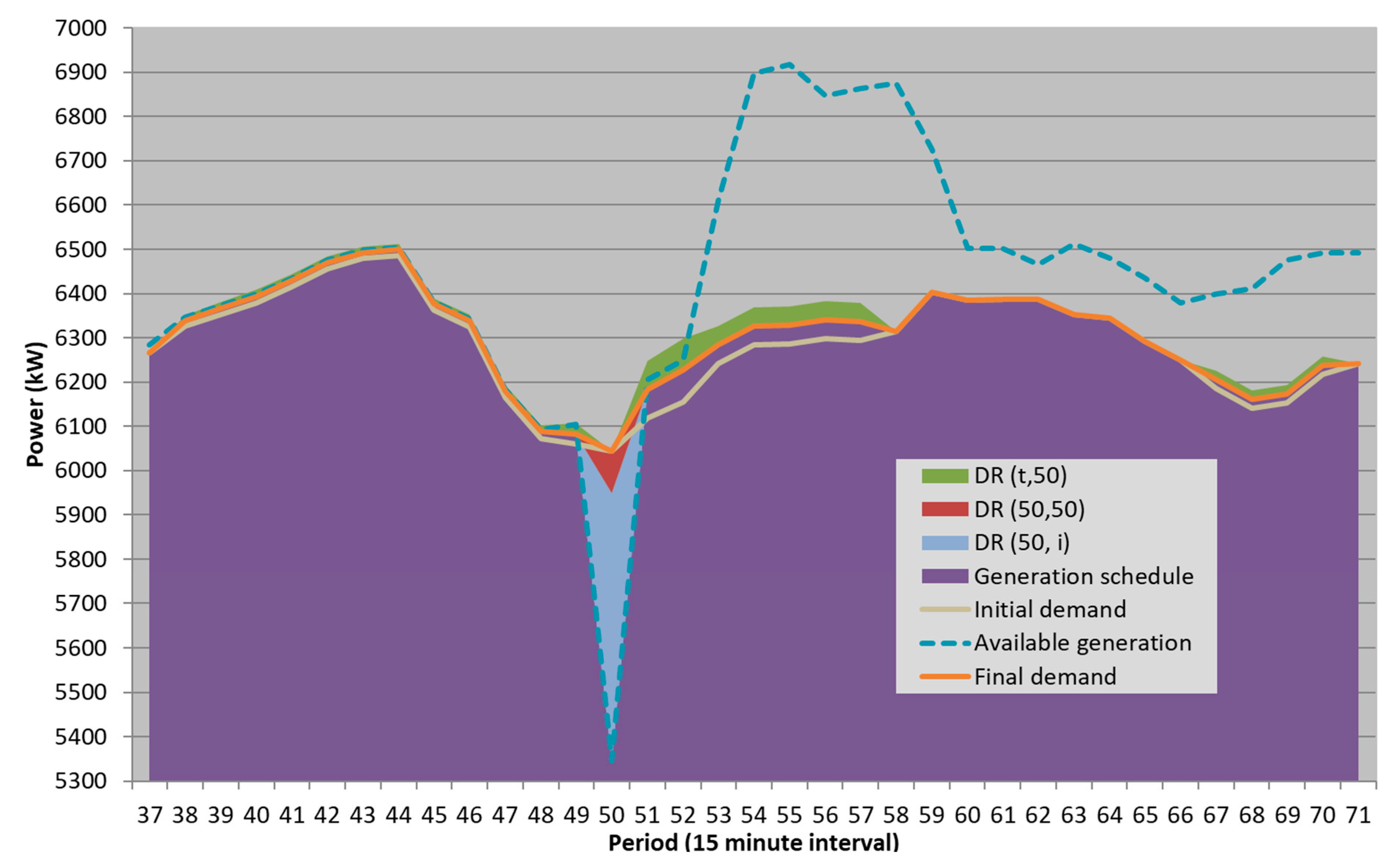
6.1. Resource’s Schedule in Scenario ScenA

Scenario ScenA is characterized by unavailability from the supply side, which brings the need for 700 kW of consumption avoidance. The obtained resources schedule is presented in Figure 5. In order to focus on the envisaged periods, Figure 5 only presents periods 37 to 71. In the legend of Figure 5 and other figures in the case study, the DR use is indicated from period t to period i, in cluster ct, when applicable. In this way, DR (t,50) refers to the consumption that is shifted from period t to period i=50; DR (50,50) refers to the consumption reduction in period 50. Finally, DR(50,i) refers to the consumption shifted from period 50 to period i.

In the light blue area, it is possible to see the 700 kW avoided consumption. It has been reduced (in red) or shifted (in green). The shifted consumption is scheduled mainly for the periods close to and after the DR event period (period 50). However, it is possible to see that some amount of consumption is shifted to later periods, as the case of period 70.

Figure 6 presents the load resources schedule for ScenA, and for consumption cluster ct2 (ct1 and ct4 were also scheduled but not presented). It can be seen the reduction (red bar) and the shift (blue bar) amounts in period 50, and the new load in each period (in purple) due to the load shifting. It is also seen the limit load reduction (dashed red line) and the shift (dashed blue line) capacity. The green area as the load shifted to each period, in all consumption clusters. The total limit of load reduction was used. A small amount of load shifting was used.

As it was explained in Section 3, the proposed methodology considers several constraints. One example of those constraints is the maximum consumption reduction in each period, for each consumption cluster. This constraint has been applied in the results shown in Figure 6. If additional consumption reduction capacity was available, it would certainly be scheduled. The use of the remaining load shifting was limited by Equation (11); αDRMax is 0.8.

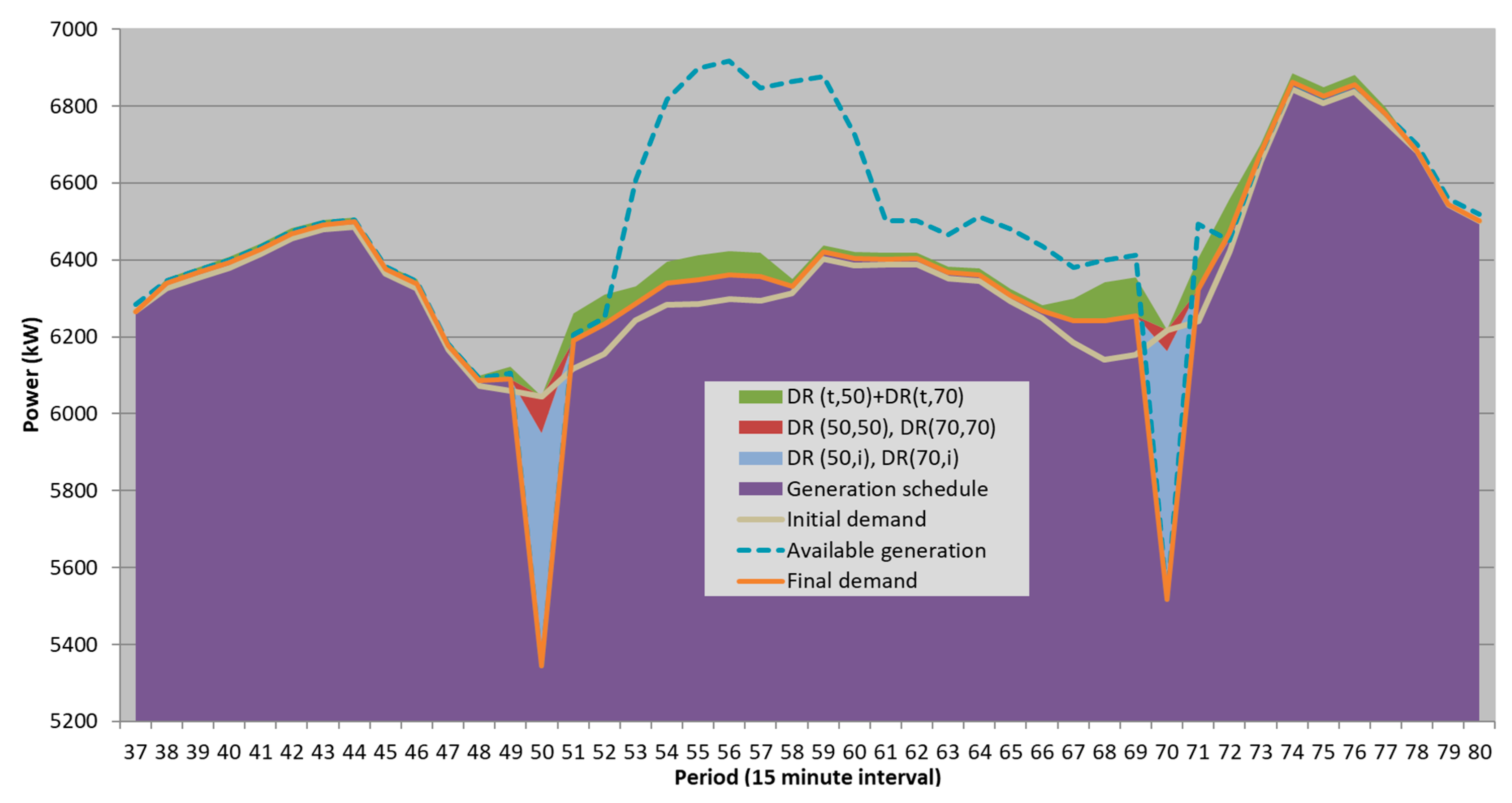
6.2. Resources’ Schedule in Scenario ScenB

This scenario considers the same supply unavailability in period 50, as in ScenA, and additional supply unavailability of 700 kW, in period 70 (between 17:15 p.m. and 17:30 p.m.).

The results for ScenB are presented for periods 37 to 80, focusing on the implemented events. Similarly to ScenA, the available supply capacity is close to the demand in the periods around period 50. The total consumption reduction in DR1 and DR2 event periods is shown in Figure 7.

As seen in section V-A, in ScenA some load was shifted from period 50 to several other periods, including those around period 70. Therefore, in the case of ScenB, it is important to discuss the impact of the DR2 event in period 70 in the resource scheduling, by comparing the results from ScenA and ScenB.

The results presented in Figure 8 make possible such a discussion. This figure presents the consumption shifted in each DR event, regarding each consumption cluster. While the load shifted in period 50 (in brown, orange and dark blue, respectively for ct1, ct2, and ct4) in ct2 and ct4 is done for close periods, for ct1 the load is shifted for distant periods. The results shown in Figure 8 concern the incoming load shifting for each period.

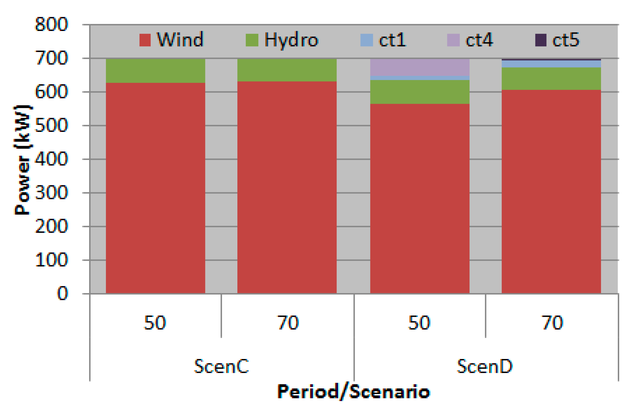
6.3. Resources’ Schedule in Scenario ScenC and ScenD

Figure 9 compares the resource scheduling for each DR event period for scenarios ScenC and ScenD. As ScenC only uses DG and ScenD uses DG and DR, these results allow making conclusions about the impact of the DR resources availability. In ScenC, all the available hydro DG is used while the wind DG is used as needed in order to reach the required 700 kW. In the case of ScenD, by introducing DR, one can see that the wind DG contribution is lower due to the use of DR for consumption clusters ct1, ct4, and ct5. In this way, the final cost has been significantly reduced.

6.4. VPP Operation Costs and DR Price Sensitivity Analysis

Let us now address the VPP operation costs for each scenario as the developed methodology aims at minimizing the operation costs. Figure 10 presents the VPP costs regarding the remuneration of the suppliers, of the DG, and of the DR (consumption reduction and shifting).

Comparing ScenA and ScenB, the operation costs are higher in ScenB due to the existence of two events of generation shortage. However, in ScenB it was possible to give less remuneration to the suppliers, distributing a part of the benefits to the consumers. Comparing ScenB, ScenC, and ScenD, all of them with two DR events, one can see that using only DG (ScenC) instead of using only DR (ScenB) leads to higher operation costs. Also when using DG and DR together for the scheduling (ScenD), the operation costs are lower than in ScenC, in which only DG is used. It is, therefore, show the advantages of using DR in alternative or together with DG.

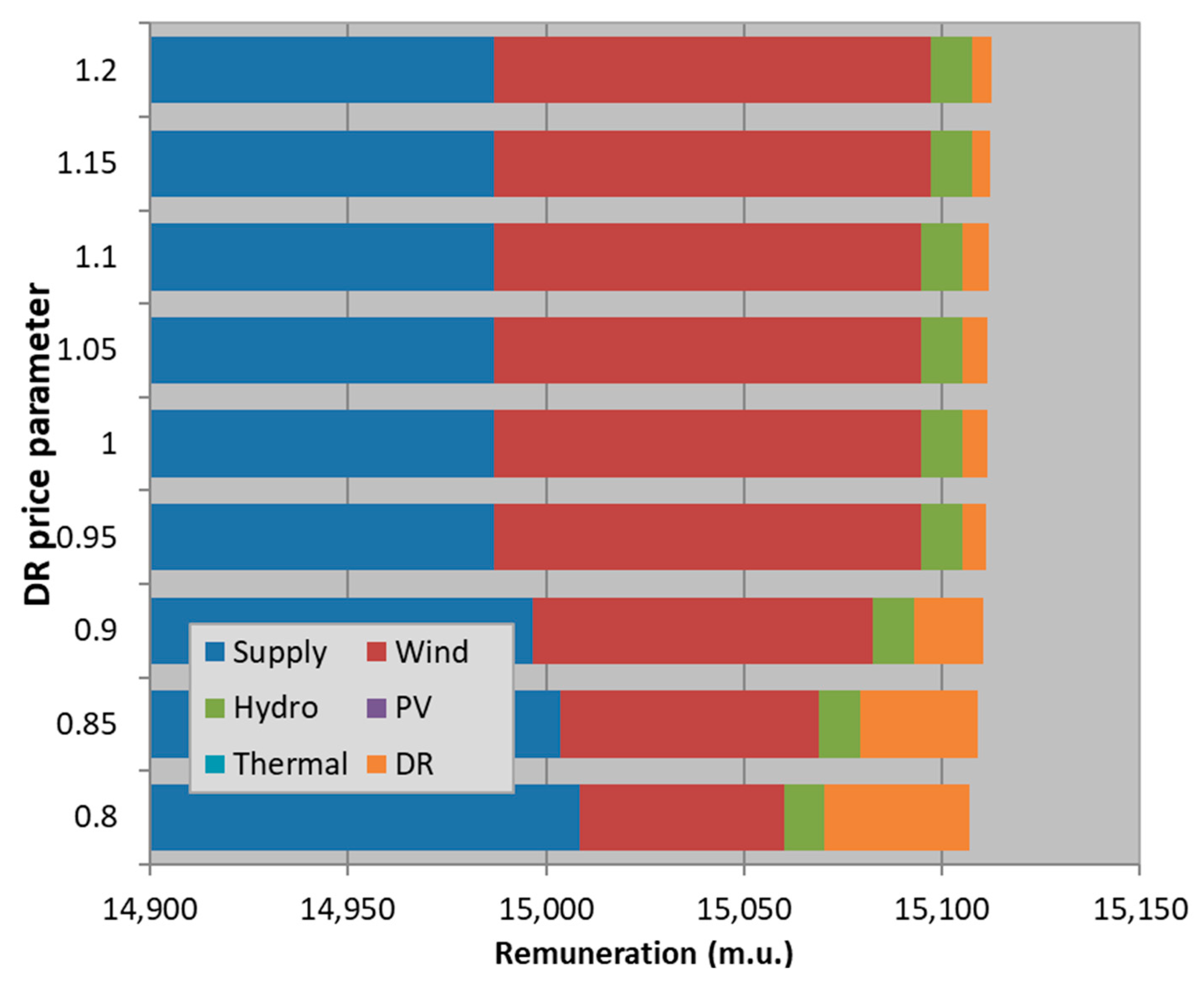
In this way, it has been possible to supply the demand avoiding the payment of high non-supplied power (NSP) costs by the VPP to the consumers, despite several consumption shifting constraints that have been implemented in the proposed model. Focusing now on the sensitivity analysis of the operation costs for the VPP concerning ScenD, and regarding the variation of the DR price, Figure 11 presents the remuneration of each resource for a variation on the DR price between 80% and 120%. This means that the prices in Table 2 have been multiplied by 0.8; 0.85; …; 1.2, according to the yy axis in Figure 11.

It can be seen that for low DR prices, the VPP operation costs are lower when DR prices decrease. In fact, a slight variation on the VPP operation costs is verified for the provided range of DR price sensitivity analysis. Moreover, DR remuneration becomes higher due to the fact that the amount of dispatched DR resources is increased. However, since the schedule is mainly based on consumption shifting, the shifted consumption will concern the remuneration of generation resources in the periods for which the consumption is shifted. For example, when the DR price is 80% of the base one (in Table 2), the use and remuneration of the supply are higher than in other DR price levels, due to the additional use of the supply related to the increased use of DR shifting. This provides proof on the flexibility that DR can provide to the management of distributed energy resources.

In order to better understand the prices and the related remuneration given to each consumption cluster, Figure 12 presents such remuneration in the conditions of the sensitivity analysis presented in Figure 11. It can be seen that with the lowering of the DR price, increasing levels of DR are scheduled. Furthermore, for lower DR prices, ct2 is scheduled and for the highest DR prices, only ct1 and ct4 are scheduled. It is important to remember that the remuneration of the resources is linearly depending on the respective price; however, according to Table 2, several distinct prices can be applied to the same consumption cluster depending on the specific scheduled DR shifting periods.

7. Conclusions

Demand response is a very valuable resource for future power systems, which will be focused on renewables and other distributed resources. In fact, DR is able to improve and increase the accommodation of distributed energy resources based on renewables. In order to reach the full potential of DR, namely for integrating distributed generation, it is needed to develop adequate modeling of DR programs and scheduling approaches.

In this paper, it is proposed the scheduling of the load shifting opportunities, performed by a VPP. The operation costs are minimized while implementing several loads and shifting constraints. The demand response approach has several dynamic input parameters. The main advantage is the modeling of the consumption shifting constraints (modeling limits for each period/set of periods) from the VPP and the consumer standpoints.

The case study focused on the integration of DG supported by DR. It has 218 consumers from five consumption clusters and four DG types. Four scenarios in two DR events were implemented. A sensitivity analysis on the VPP operation costs regarding the variation on the DR price has been performed, addressing also the remuneration of each consumption cluster. It has provided proof on the flexibility that DR can give to the operation of distributed energy resources, namely when considering the integration of renewables.

Concerning the advantages of the proposed method, one can say that when declaring a DR event, due to a shortage from supply resources, consumers can reduce the load by shifting part of that to other periods, benefiting with the remuneration of actual reduction in the DR event. It has also been proved the advantage of considering DR in spite of using only DG in the generation shortage periods. In this way, the VPP avoids paying for the non-supplied power. Therefore, the VPP is able to give the consumers the opportunity of modeling their behaviour in what concerns the consumption reduction and shift, increasing the advantages for both VPP and the consumers.

As future work, some aspects can be considered in order to proceed with the work here presented, namely considering different methods in the optimization, modeling uncertainty of DG and DR resources, adding more constraints to the modeling of resources, and elaborating on the aspects related with the load forecasting.