A Time-Series Data Analysis Methodology for Effective Monitoring of Partially Shaded Photovoltaic Systems

Abstract

The majority of photovoltaic (PV) systems in the Netherlands are small scale, and installed on residential and commercial rooftops, where different objects in many cases may lead to the presence of shading and inevitable energy loss. Nevertheless, the energy loss due to expected shadow must be distinguished from the energy loss due to other malfunctions. In this study an algorithmic tool is presented that automates the process of analyzing monitoring data of partially shaded PV systems. The algorithm compares long-term and high-resolution yield data of a partially shaded PV system with the yield data of an unshaded PV system, as reference PV system, and automatically detects the energy loss due to the expected shadow, caused by any surrounding obstacles, and distinguishes it from any additional energy loss due to other malfunctions. This study focuses on PV systems with module-level power electronics (MLPE) since these are mostly used on PV systems on rooftops. Three different cases of shaded MLPE PV systems are presented to illustrate the versatility of the methodology. Furthermore, suggestions for further research are discussed at the end of the paper.

1. Introduction

1.1. Research Motivation

Photovoltaic (PV) installed capacity worldwide has remarkably increased the past years, from 25 GW in 2008 to 500 GW at the end of 2018 [1], and the Netherlands is catching up too, from 59 MW in 2011 to 4.2 GW in 2018 [2]. At the end of 2016, 70% of the installed capacity was on rooftops [3], a condition which continued during 2017, since 49% of new installations were on residential and 46% on commercial rooftops [2], neither during 2018, where 38% of the new installations were on residential rooftops [4]. With a continuously increasing urban population, the percentage of PV systems on rooftops is forecasted to keep growing in the future, as the European Commission has been promoting the increase of residential PV systems from 2010 onwards with the Energy Performance of Buildings Directive (EPBD), which provides guidelines towards the realization of net zero-energy buildings [5].

The complexity of the urban environment is challenging for the deployment of PV technology, especially on rooftops, where different objects, like poles, antennas, and dormers may be present that obstruct the irradiance reaching PV modules and thus affecting their energy output [6]. For example, a recent study shows that PV systems installed in urban environments are performing worse compared to ones installed in rural environments [7]. Furthermore, the performance of the urban PV systems is reducing in areas with higher building density and higher average building height [7].

Clearly, shadow is one of the main reasons of lower performance of residential PV systems; however, it is not the only one, since the performance of the PV systems is also depending on their condition and on operational issues leading to energy loss [8]. Any operational problems must be detected fast to limit the associated energy loss. As a consequence, monitoring of PV systems is an important topic for scientists and owners of PV systems, as it can give insights in the operation of systems and their performance, while it also allows detecting any malfunctions that may occur.

Different PV monitoring methods have been developed in the past years. The main principle on which these methods are based was either the comparison of the produced energy with the available solar radiation or the simulation of the produced energy, based on the available solar radiation and its comparison with the real production. The strong majority of the proposed models shows impressive results, especially on malfunction detection on PV plants, see Section 1.2 for details. However, as mentioned above, PV systems on rooftops differ due to their surroundings in the urban environment, and a detected shadow may not be characterized as a malfunction and raise an alarm in an automatic malfunction detection algorithm, since, in the strong majority of the cases, it is created by objects which cannot be removed, such as chimneys, poles, or other buildings. Additionally, any other operational problem should be detected as fast as possible and raise an alarm.

In this paper an algorithmic tool is developed, that automatically detects the energy loss due to the expected shadow, expected since it is caused by any (unremovable) surrounding obstacles and distinguish it from any additional energy loss due to other malfunctions. The algorithm focuses mostly on systems that consist of micro inverters or power optimizers, and unshaded panels are used as reference data.

1.2. Literature Review

1.2.1. PV Monitoring and Malfunction Detection through the Years

As mentioned in the introduction, in the past years, different PV monitoring methods have been introduced. Their main principle was either the comparison of the produced energy with the available solar radiation or the simulation of the produced energy, based on the available solar radiation and its comparison with the real production. The first was introduced at the end of the 90’s with the introduction of the performance ratio [9]. During the 00’s, more complicated methods were introduced, either by using the solar irradiance and other weather conditions to simulate the PV production in 2005 [10], or by using the performance ratio together with malfunction patterns in 2006 [11] and 2007 [12].

After 2010, due to the sharp increase of the global penetration of PV systems, more and more malfunction detection methods, based on these principles, were introduced. Firth et al. [13] in 2010 introduced a simple PV system performance model and applied it for malfunction detection. Similarly, an automatic supervision and fault detection procedure for PV systems, based on analysis of power losses, was introduced [14].

Between 2012 and 2013 Silvester, Chouder et al. introduced a new, quite accurate, simulation model for malfunction detection in a series of articles [15,16]. The same year Eke and Senturk [17] used solar, meteorological data and reference systems in order to monitor building-integrated PV systems (BIPV) and observe and report occurrences of energy loss due to higher operating temperature of the modules. Moreover, in 2013 an automatic fault detection method for grid-connected photovoltaic (GCPV) plants was introduced, which generates a diagnostic signal that indicates possible faults occurring in the GCPV plant and monitors the DC to AC power ratio in order to determine the location of the fault [18].

In the framework of IEA-PVPS (International Energy Agency-photovoltaic Power Systems Program) TASK 13 [19], a report was released [8] on monitoring and malfunction detection where characteristic scatterplots of different malfunctions are presented. The collection of plots (named “stamp collection” in the report) aims to help in the identification of malfunctions on PV systems by visual comparison.

In 2015, a new algorithm for the modeling of the DC side of the PV array was introduced [20]. The same year, Platon et al. [21] proposed an online monitoring method, where the real production of the monitored PV systems was compared with modeled data, obtained by a model similar to one used in [12]. In 2016 a new fault detection algorithm for photovoltaic plants was introduced [22], able to detect different types of faults on the DC. Furthermore, a method based on data mining techniques has been introduced, to predict faults or special conditions that occur due to shadows, bad weather, soiling, and technical faults [23].

In 2018, two new methods were introduced for automatic fault detection, one by monitoring identical sets (sister arrays) connected to the same inverter of PV system [24] and one where PV measurements are clustered to normal and non-normal operation, based on the historical behavior of the PV system [25]. A most recent study featured the use of drones for temperature monitoring of PV plants on large rooftops [26].

1.2.2. Shadow Detection and Its Impacts on PV Performance

As mentioned in the introduction, shading is one of the main reasons of lower performance of residential PV systems, thus different studies have been conducted on its impact. Mohammedi et al. [27] studied the impact of shadow on the performance of a domestic photovoltaic pumping system incorporating an MPPT control and proposed different array configurations which show different behaviors in relation to partial shading conditions. Sinapis et al. [28] studied the effect of the same shading on three PV systems with the same panels but different system designs (one system with string inverter, one with power optimizers, and one with string inverters). Based on the same system a simulation model was developed to quantify the benefits and drawbacks of different PV system architectures, which includes a shading evaluation of the installation based on 3D modeling, irradiance calculations, and PV and cell modeling [29]. Similarly, a model for detecting an optimal PV system configuration for the given installation area is introduced in [30], where the effect of the interrow shading is modeled. Another method able to identify anomalies, such as shadow, by comparing the I-V curve in normal operation and the I-V curve in shading condition was presented in [31]. A different approach of shading detection, since it is taking place on the direct current (DC) side, was proposed at [32]. Another different approach is presented in [33], where a shadow identification and prediction method based on PV system and local weather data, processed by the support vector machine (SVM) shading model is introduced. LIDAR (light detection and ranging of laser imaging detection and ranging) has been used as well in a LiDAR-based model for shadow identification [34] with quite promising results. Unique data shows the effect of a solar eclipse, on a PV system installed on a complicated rooftop [35], and could be compared with the pattern of a shadow during a sunny day.

1.3. Research Purpose and Paper Organization

1.3.1. Research Purpose

The purpose of this paper is to introduce an algorithmic tool which will automate the process of analyzing monitoring data of partially shaded PV systems. The main goal is to detect the period where a PV system is affected by partial shadow and distinguish the caused energy loss from the energy loss that is caused by other malfunctions.

The approach of the algorithm is to compare long-term and high time resolution yield data of a partially shaded photovoltaic system (referred to as “studied PV” for now on) with reference data (yield of an unshaded PV system or the tilted irradiance, referred as “reference data” from now on). Firstly, the moments where the studied PV is not operating normally were detected and then their occurrence during the day was studied. If non-normal measurements constantly occurred at a specific time of the day, for that certain period the algorithm characterized them as shadow.

1.3.2. Paper Organization

This paper is organized as follows. Section 2 discusses the scope of the algorithm, its limitations, the necessary data preparation in order to operate effectively, and the PV system where the algorithm is tested. Section 3 provides the description of the proposed algorithm in four different steps and the verification of the algorithm with the use of diffuse horizontal (DHI) and direct normal irradiance (DNI) data. In Section 4, the algorithm is applied to two different systems under different shading conditions and the results are discussed. Finally, Section 5 summarizes the main findings of the paper.

2. Scope, Limitations and Data Preparation of the Algorithm

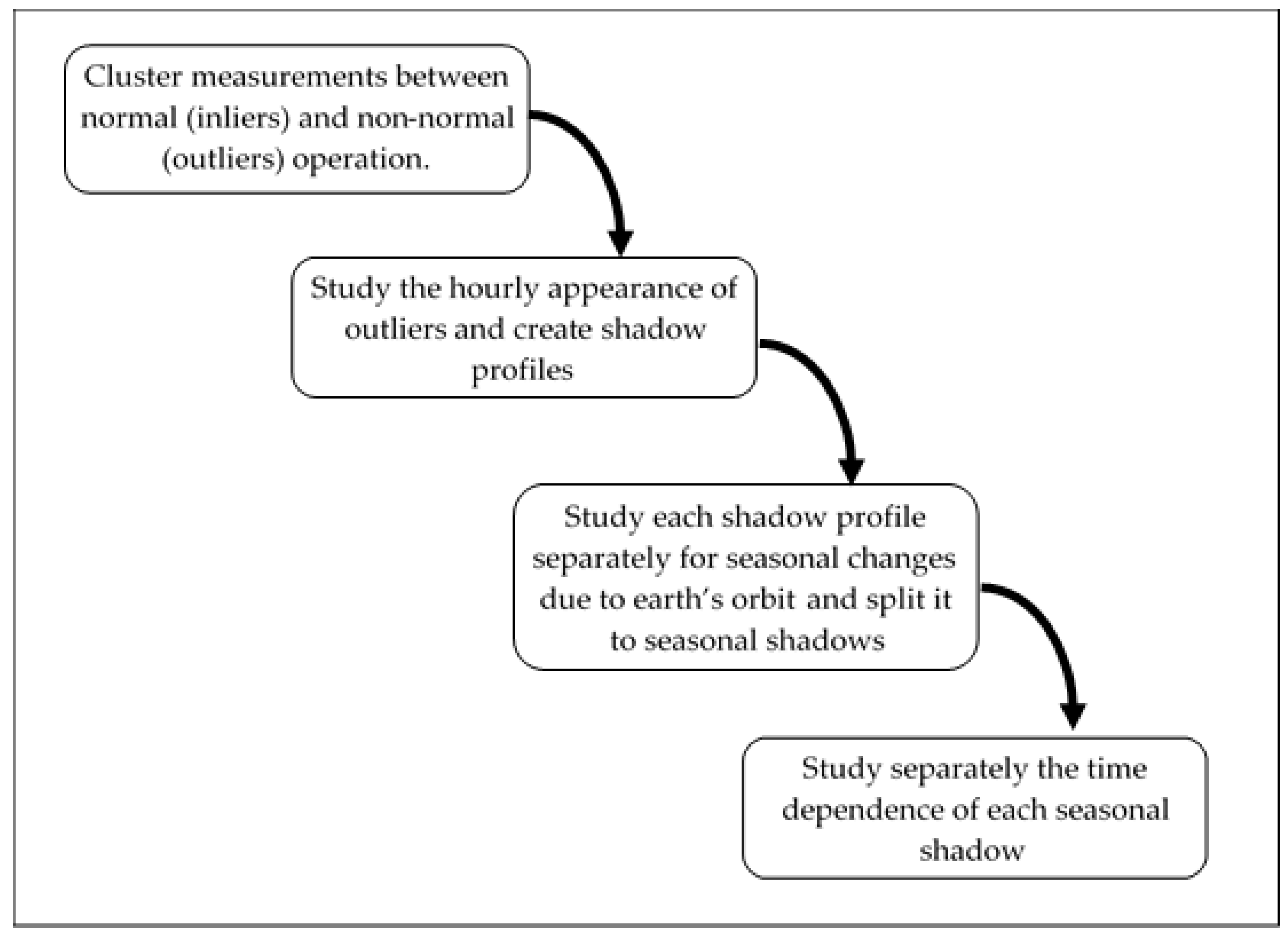
2.1. Scope of the Algorithm

The basic principle of the proposed monitoring method is to study the daily persistence of any occurred error between the studied PV and the reference PV data, identify the daily repeated errors, characterize them as shadows, and make a profile for every shadow which affects the system. With the combination of all the shadow profiles, the algorithm creates the “shadow story” of the studied PV (i.e., a table with the starting and ending dates of the shadow(s) during the year and the expected starting and ending times of the shadow(s) during each day). Any difference between the yield of the investigated PV and the reference PV system, outside of the limits of these shadow profiles, is characterized as a malfunction and within these profiles as shadow. Thus, the beginning and ending date-dependent times of each individual shadow is called the profile of the shadow or shadow profile and the combination of all shadow profiles is the shadow story of the studied PV system.

The algorithm followed the following four steps:

• Define a threshold of the error, to distinguish between normal and non-normal operation.
• Study the hourly appearance of non-acceptable errors.
• Study the shadow profile for seasonal changes in the start-end time of the shadow.
• Study, separately, the time dependence of each shadow profile.

These steps are explained in the following Section 3.1, Section 3.2, Section 3.3 and Section 3.4. Each section contains two subsections. In the first subsection (3.X.1) the principle of the step is explained. In the second subsection (3.X.2) the step is applied to a shaded PV system and it is visualized for better understanding. In the example, normalized power production of a neighboring panel with power optimizer is used as reference data. In the remainder of this section, we describe limitations and data collection.

2.2. Limitations of the Algorithm

2.2.1. The Dependence of Shadow on the Irradiance Conditions

The purpose of the algorithm is to detect shadows created by obstacles which are present on rooftops (i.e., chimneys, dormers, exhaust pipes). Although such obstacles are constantly present at or close to the location of the PV system, depending on the irradiance conditions, they may not create shadow on a daily basis, since the existence of a shadow is depending, as well, on the irradiance conditions. Shadow is mainly created when the direct irradiance component is blocked by an obstacle, and the corresponding reduction in energy generation can more or less easily be detected. However, in cases where the diffuse component of irradiance is high compared to the direct one, the difference in the energy generation between a shaded and an unshaded PV system could well be negligible.

An example is shown in Figure 1, where the production of two identical neighboring solar panels with micro inverters are compared. One panel was shaded (blue line) in the morning. In the left plot, a day of clear sky conditions, the difference in the production due to the shadow is very obvious. On the other hand, the day after, on the right plot, under non-clear sky conditions, the difference in the production was negligible. Thus, shadow cannot be defined as pattern, since depending on the weather and the period of the year zero existence of shading induced reduction of power may occur for several consecutive days.

2.2.2. Error Outside Shadow Characterized as Potential Malfunction

As will be described in Section 3, the algorithm detects the presence of an error at a specific time period of a day for consecutive days and characterizes it as shadow. Any occurred error outside of the periods characterized as shadows is then characterized by the algorithm as a malfunction due to other reasons.

2.3. Data Preparation

Two different sets of data are required for the development and validation of the proposed method, the power output (either DC or AC) of the studied PV system (referred to as “studied PV” from now on) and the reference data (referred to as “reference data”). The reference data could be the power output (either DC or AC) of a neighboring PV system, with same tilt and orientation (also known as peer-to-peer (P2P) comparison) or the tilted irradiance measurements from a pyranometer (global tilted irradiance, GTI), reference cell, or calculated tilted irradiance from satellite-based measurements.

Before the algorithm can be applied, both data samples should be pre-processed into a specific form in order to create a linear relationship in a scatterplot “studied PV vs. reference data”, in which the system yield Y_f is plotted versus the reference yield Y_R. The process depends on the type of reference data, whether it is solar irradiance, or the production of a neighboring PV system. System and reference yield are defined as:

$$Y_f=\frac{E_{AC}}{P_r} \left[\frac{\mathrm{k}\mathrm{W}\mathrm{h}}{\mathrm{k}\mathrm{W}\mathrm{p}}\right],$$

(1)

$$Y_R= \frac{GTI}{1000} \left[\frac{\raisebox{1ex}{$\mathrm{W}\mathrm{h}$}\!\left/ \!\raisebox{-1ex}{${\mathrm{m}}^2$}\right.}{\raisebox{1ex}{$\mathrm{W}$}\!\left/ \!\raisebox{-1ex}{${\mathrm{m}}^2$}\right.}\right],$$

(2)

in which E_AC is the AC energy generated in kWh and P_r the rated PV capacity in kWp. In

Table 1. The mandatory preprocessing of each data set. Y_f and Y_R are calculated from Equations (1) and (2). P_studied and P_ref are the rated capacity of the studied PV system and the reference system, respectively. Y_f,studied and Y_f,ref are the yields of the studied and reference system.

	Reference Data	GTI	Neighboring PV System
Data			Same Capacity	Different Capacity
Studied PV		Yf	Pstudied (DC or AC)	Yf,studied
Reference data		YR	Pref (DC or AC)	Yf,ref

the mandatory data preprocessing is presented, depending on the reference data and studied data. For instance, if the reference data is GTI then the refence data should be in form of Y_R and studied PV in form of Y_f. If the studied and reference data are PV systems with same capacity (like in a MLPE system) then their power or energy production is used.

2.4. Data Source

The proposed method was applied using data from the testing facility of SEAC (Solar Energy Application Center, Eindhoven, the Netherlands). Data from two PV systems of the facility are used, with identical panel structure (six panels in two rows, one front, one back, same tilt and orientation) and different inverter technology [28,29]. In Figure 2, a photograph of the system is presented. The used systems are the ones on the right-hand side, equipped with six micro inverters (265 W each) and the system on the left, equipped with six power optimizers connected in parallel (boost DC/DC) and a central inverter of 1.5 kW especially made for the power optimizer system. In front of each system a pole is placed (same dimension for every system) in order to create an artificial shadow on the front rows of each system during the day which is equal for all systems. Furthermore, DHI (diffuse horizontal irradiance), DNI (direct normal irradiance), and GHI (global horizontal irradiance) measurements are available, measured at Technical University Eindhoven, approximately 4.5 km from the testing facility and the GTI, in the plane of array, through two pyranometers mounted next to the PV systems.

3. Description of the Algorithm

In this chapter the algorithm is described and visualized for better understanding. As an example, the production data of a shaded solar panel with power optimizer is used. The panel was shaded by a pole in the morning and the pole was placed in front of the panel during two different periods, from April 21 to May 6 and from August 8 to October 13. After October 18 the panel was shaded early in the morning by the wall in front of the system (see Figure 2). As reference data, the panel with the highest production from the unshaded panels in the back row is used.

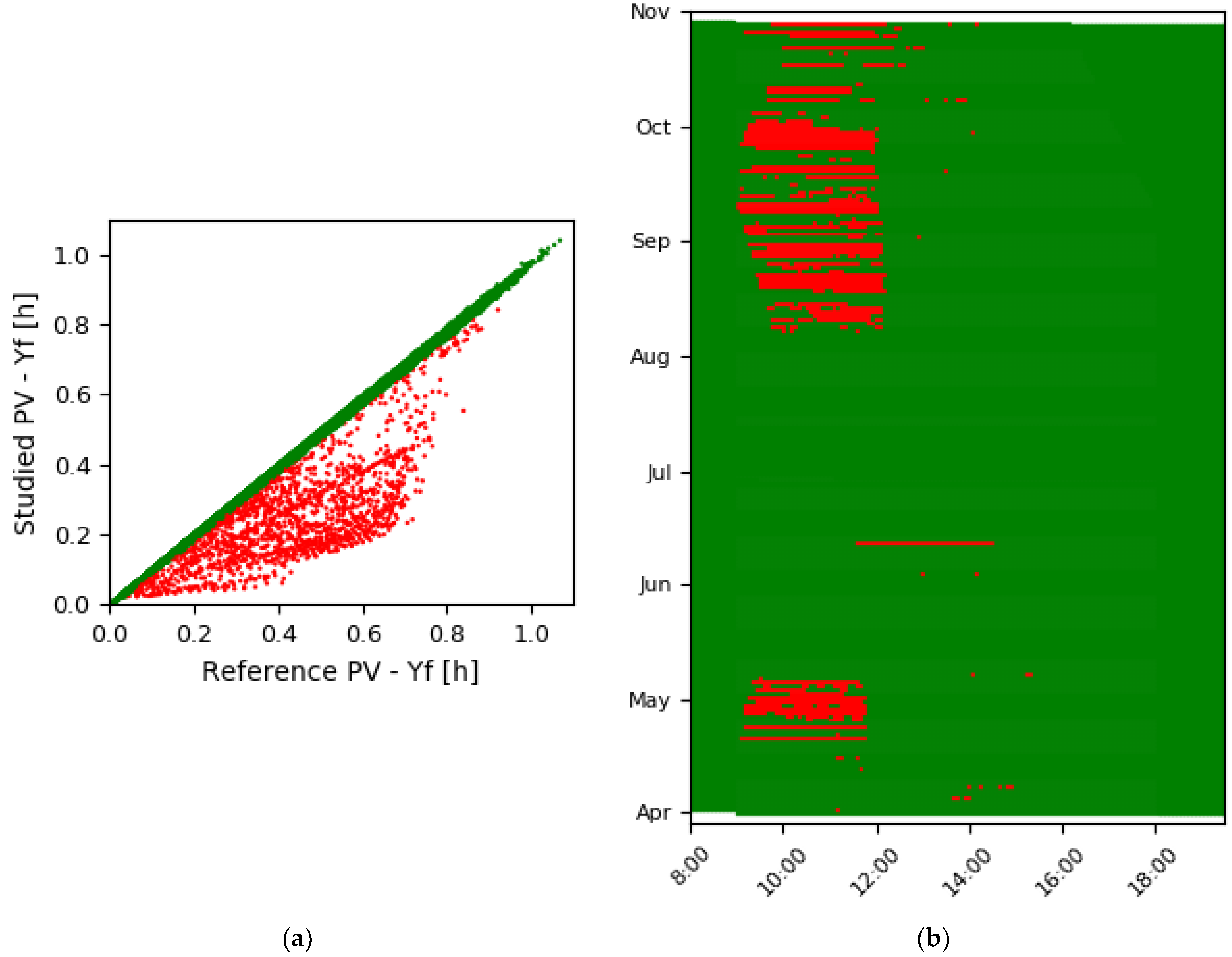
3.1. Step I, Define the Outliers

3.1.1. Explanation of Step I

The starting point of the first step is the application of an algorithm that we have developed previously [25]. This method is based on proper clustering of data and has proven to be able to detect and isolate those moments in time where measurements show that a system is not operating properly.

In this step, after the application of the clustering algorithm, the power of the studied PV is compared with the reference data and the measurements are divided into inliers and outliers. The inliers are the measurements which are following a relationship between the studied PV and the reference data which tends to be linear, while the outliers are the measurements which are not following this relationship, thus the moments where the studied PV is not operating properly. In this paper these measurements will be studied further in the next steps.

3.1.2. Application and Visualization of Step I

The clustering algorithm, as detailed in [25], is applied to the dataset and clusters the data to inliers and outliers. In Figure 3a an example is presented, where the green markers are the inliers and the red markers the outliers, which will be studied in the next step of the algorithm.

After the application of the clustering algorithm the measurements are plotted, as well, in a time versus date plot, for a better overview of the apparent faults of the PV system. Such a scatterplot is presented in Figure 3b, where the measurements of Figure 3a are plotted based on the date and time of their occurrence and colored based on their characterization as inliers (green) or outliers (red). It is obvious that the outliers are concentrated around specific periods (i.e., at the beginning of the day). The aim of the next steps is to automatically detect and isolate these periods, thus finding the profiles of each shadow (i.e., the shadow profiles).

3.2. Step II, Hourly Occurrence of Outliers—Detect Shadows

3.2.1. Explanation of Step II

As described in Section 3.1, the moments at which the studied PV system is not operating normally are detected. In step II the frequency of appearance during the day is studied. The timestamps at which the frequency of outliers is high are characterized by the algorithm as shadows and the beginning and ending moment of each shadow are characterizing the “profile of the shadow”. Thus, errors within shadow profiles are characterized as shadows while errors outside the shadow profile as malfunctions.

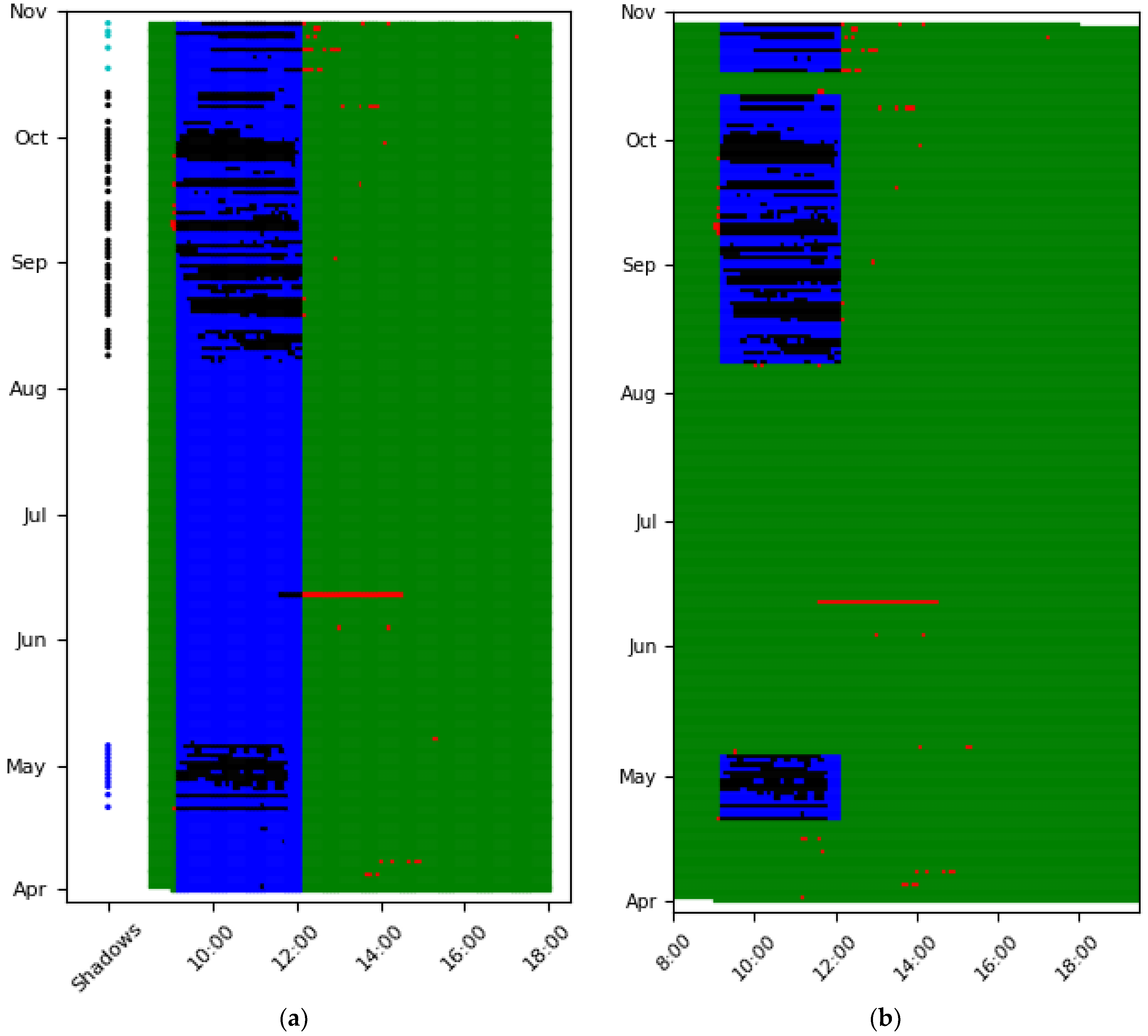
3.2.2. Application and Visualization of Step II

In Figure 4, step II is visualized for better understanding. The graph represents the distribution of the outliers during the day. Between 9:00 and 12:20 the frequency of appearance of outliers is higher than the average and is reordered as shadow profile.

During the detected shadow profile, quite a few inliers are detected as well due to the high diffuse irradiance, as is explained in Section 2.2.1.

For better understanding the measurements can be presented in a time vs date scatterplot (as in Figure 3), whereby measurements are color-coded depending on their relationship with the detected shadow profiles and their clustering as inliers or outliers during step 1, as follows:

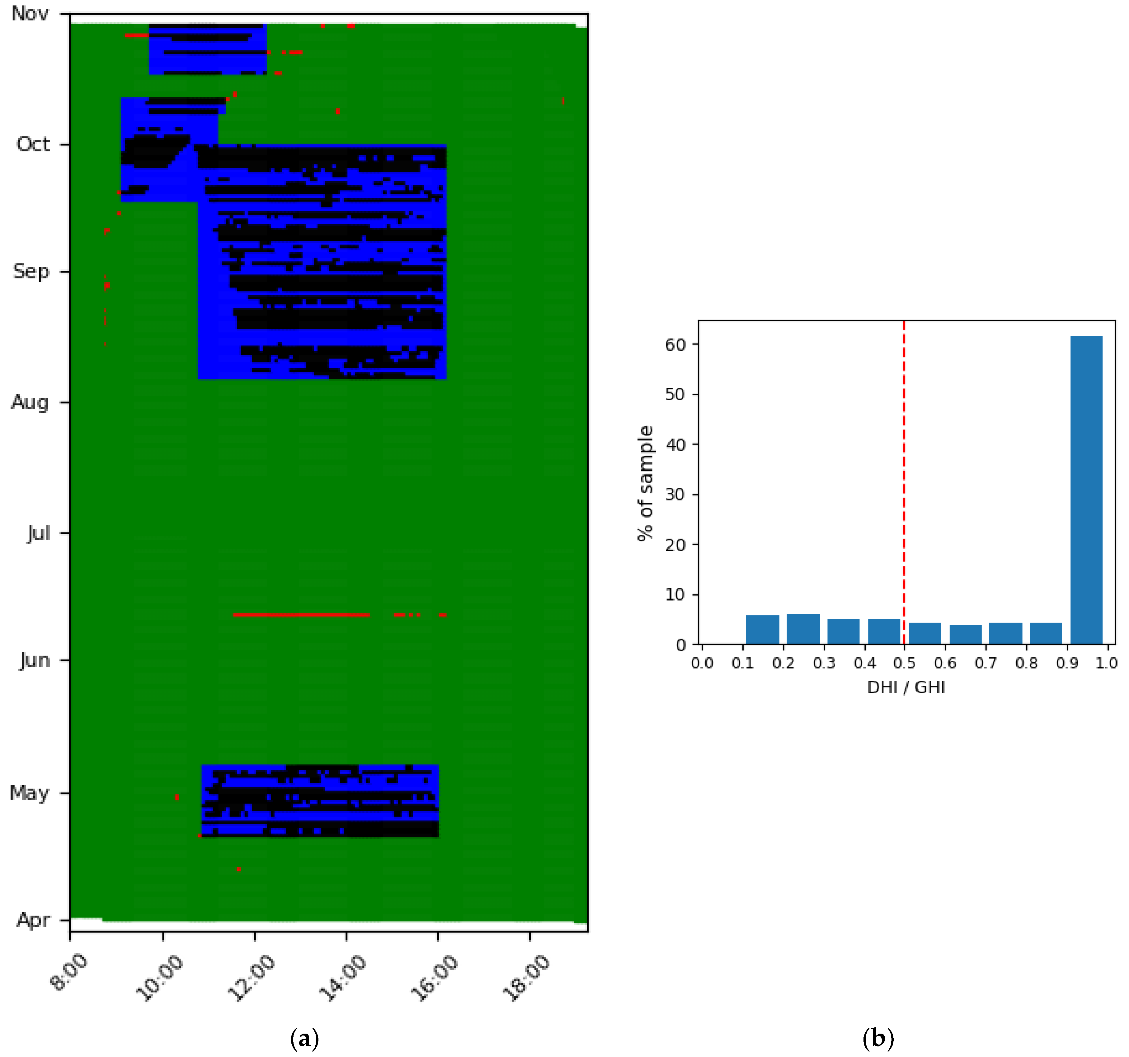
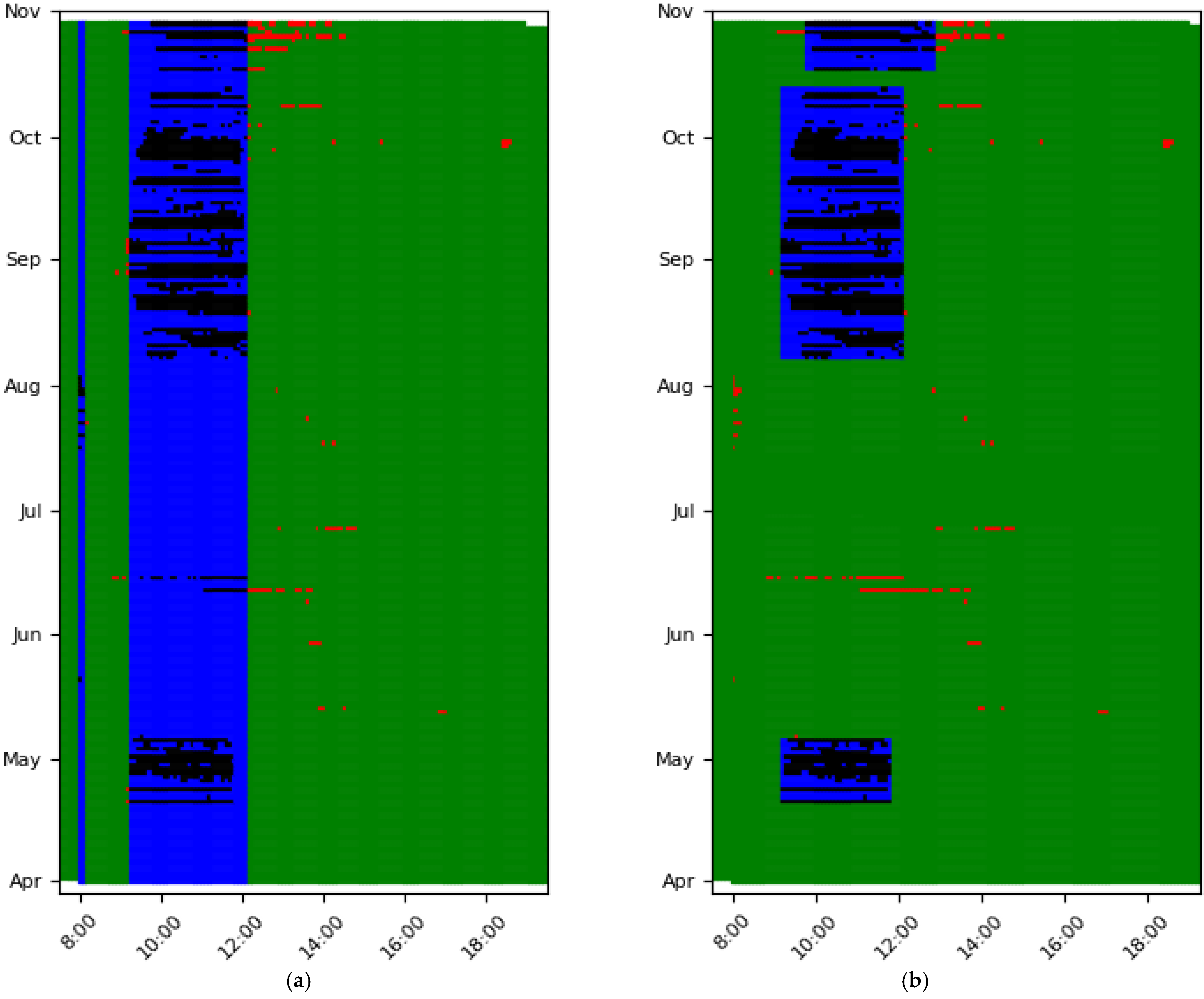
• Green: Inlier outside of shadow profile
• Blue: Inlier within shadow profile
• Black: Outlier within shadow profile, thus shadow
• Red: Outlier outside shadow profile, thus other malfunction

In Figure 5 an example is presented whereby the data in Figure 3 is re-color-coded, based on the shadow profile detected in Figure 4.

3.2.3. Discussion of Step II

At the end of step II, any shadow profile(s) is detected. Thus, all the outliers outside the shadow profile(s) are characterized as malfunctions and within them, shadows. Furthermore, as can be seen in the example of Figure 4 and Figure 5, many inliers are within the shadow profiles as well and the explanation lies in the nature of the diffuse irradiance, as it is explained in Section 2.2.1.

Nevertheless, in the presented example the pole which creates the morning shadow was removed during summer months. However, the algorithm at the end of step II expects a shadow in these months and any errors that occur, such as the presence of a cleaning crane in mid-July, is partially recognized as shadow, even if is a malfunction, since it was shadow but from an unexpected object and lasted only for a few hours. Due to this fact it is essential that each detected shadow profile should be clustered to shorter periods during the year and the presence of the outliers during the day should be studied again.

3.3. Step III, Cluster Dates in to Smaller Groups

3.3.1. Explanation of Step III

In the third step the detected shadow profile(s) detected in step II is/are further studied in order to overcome the problems mentioned in Section 3.2.3. In case of more than one detected shadow profile, each shadow profile is studied separately, since they are or may be created by different objects and different time periods during the day.

In step III the dates of the profile(s) are characterized as being part of the shading profile if more than half of the measurements inside the profile have been characterized as outliers during step I. The clustering method DBSCAN (density-based scanning) [36] is applied only on days with high presence of shadows, and clusters these in smaller groups of days. The start and ending dates of each group are used to divide the shadow profile into smaller date periods. Furthermore, DBSCAN prevents any overlapping between these periods.

3.3.2. Application and Visualization of Step III

In Figure 6 step III is visualized. In the presented example, during step II, one shadow profile has been detected. In step III, only the days with high presence of shadow are used as input to DBSCAN, which is applied as many times as the detected shadows, one for the case of the example. In Figure 6a, the colored dots on the left of the plot are representing the dates which are used as input of DBSCAN and have been clustered in three different groups, as presented by the different colors. Dates which are not assigned in the group are characterized from DBSCAN as outliers and are not presented in the plot. In Figure 6b the result of applying DBSCAN is shown. Faults only within the dates recognized as shaded from DBSCAN are characterized as shadows. Especially the individual fault in mid-June is now characterized as malfunction (colored red) and not as shadow, as (part of it) in Figure 6a.

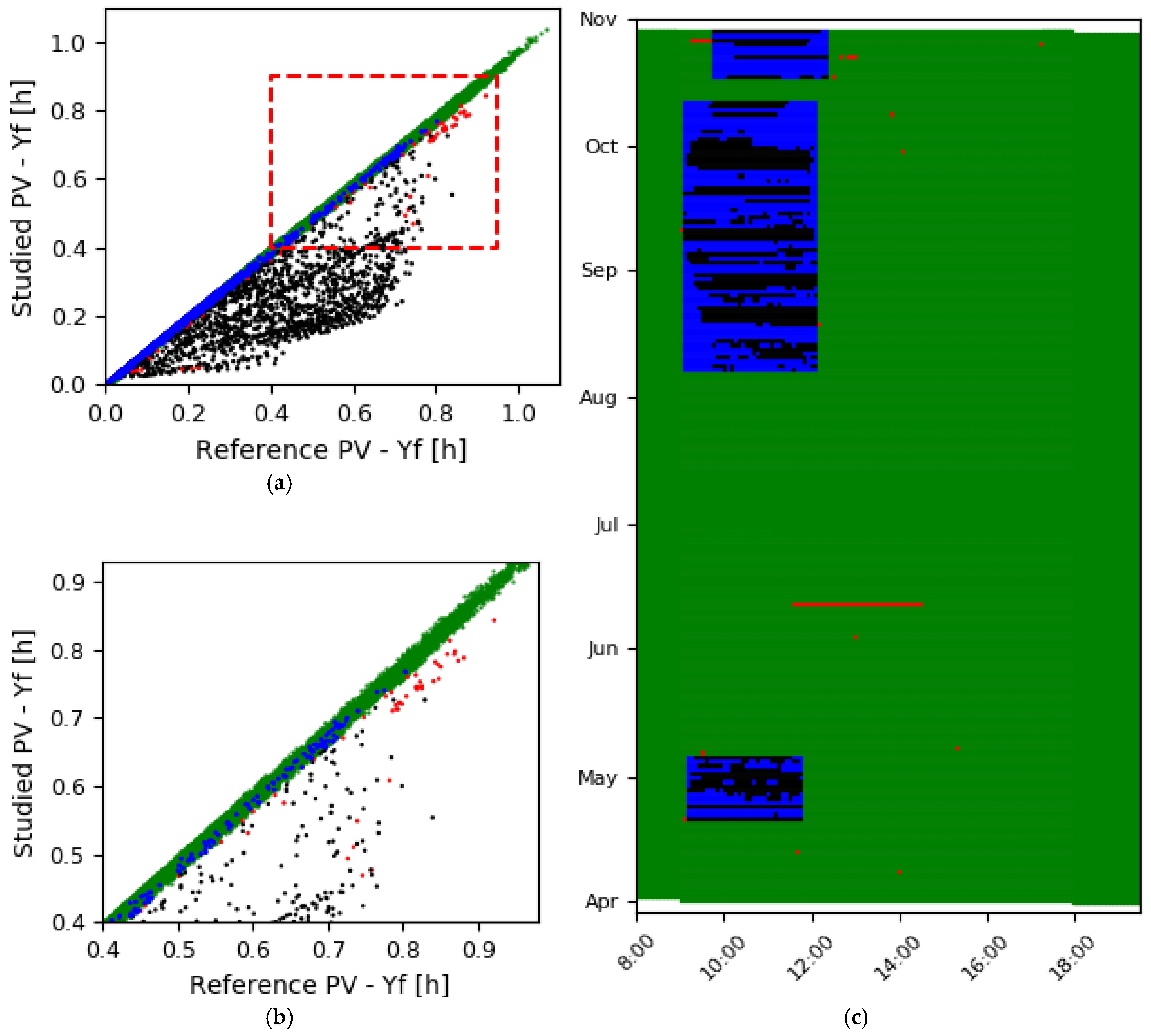
3.4. Step IV, Second Hourly Distribition

3.4.1. Explanation of Step IV

As described in step III, each shadow is clustered to different date groups. In step IV, each of these groups is studied separately with the application of Step II, not for the whole day (as in step II) but only within the limits of the shadow profile with an extension of 30 min before and after the profile. Thus, in every group, the moments with errors higher than the threshold are characterized as faults and their appearing frequency during the extended limits of the shadow profile is studied. The moments where the faults are more than the total measurements are characterized by the algorithm as shadows and the beginning and ending moment is the characteristic shadow profile of the group. The purpose of this act is to detect and map the differences in the start and the end times of the shadow during the year due to Earth’s orbit around the sun.

The final outcome of the process is a table which is called “shadow story” and demonstrates the change of the shadow effect during a long-time studied period. In the final table, each shadow is divided in different date periods (without overlaps) and for each period the starting and the ending time are provided.

3.4.2. Application and Visualization of Step IV

In

Table 2. The detected shadows of the example. Each row represents a shadow profile. It contains information about the start and end date and time of the shadow. The table with all the shadows that are affecting the system during the studied period is called “shadow story” and it is the final outcome of the proposed algorithm.

Detected Shadow
Shadow Profile	Dates		Hours
	from	to	from	to
1	21 April	6 May	9:10	11:45
2	8 August	13 October	9:05	12:05
3	18 October	29 October	9:45	12:30

the shadow story of the example is presented. Furthermore, in Figure 7c, the final version of the time vs date scatterplot is plotted. Clearly, in this version the beginning and end times of the shadow are changing during the year. Furthermore, shadows are not expected during unshaded periods, thus the maintenance at mid-June is completely recognized as a malfunction.

Additionally, the impact of the fourth step can be strongly noticed at the starting and ending times of the third shadow profile (Table 2). In contrast with the other two, these times are 30 to 45 min later. As depicted in Figure 5b and Figure 6, initially the algorithm expects this shadow, caused by a small wall, to be the same with the one from the pole (shadows 1 and 2 in Table 2). However, after step III, starting and ending times are observed to be date dependent (as can be seen in Figure 6b), which is clearly detected in step IV. These differences are due to the fact that the impact of the wall on the system is date dependent.

A consequence of step IV is the adjustment of the scatterplot studied PV vs reference PV, shown in Figure 7a. Compared to Figure 5a, the number of blue markers is significantly less at higher energy values, which, in fact, is more clearly visible in Figure 7b, which is a zoomed-in part of Figure 7a. Finally, the flowchart of the process is presented in Figure 8.

3.5. Verification of the Method

As depicted in Figure 7c, within the time intervals of the shadow story, there is a large number of measurements where an error is expected but not observed (blue markers). It can safely be assumed that this is due to high diffuse irradiance, which, in contrast with the direct, is not obstructed by the shade causing object, as explained in Section 2.2.1. In Figure 9, the ratio of diffuse to direct irradiance is presented in a histogram, only for the blue markers of Figure 7c. It is clear that for the strong majority of the measurements where the expected shadow is not observed, the DHI was the dominant irradiance component. For 82% of the measurements, the DHI was the dominant component, since its ratio to GHI was higher than 0.5 (on the right-hand side of the red line in Figure 8). Moreover, for 65% of the blue markers in Figure 7c, the DHI was more than the 90% of the GHI. Thus, the existence of the shadow in those cases is unfeasible.

4. Results

In this section, some examples of application of the algorithm are shown to illustrate its usefulness.

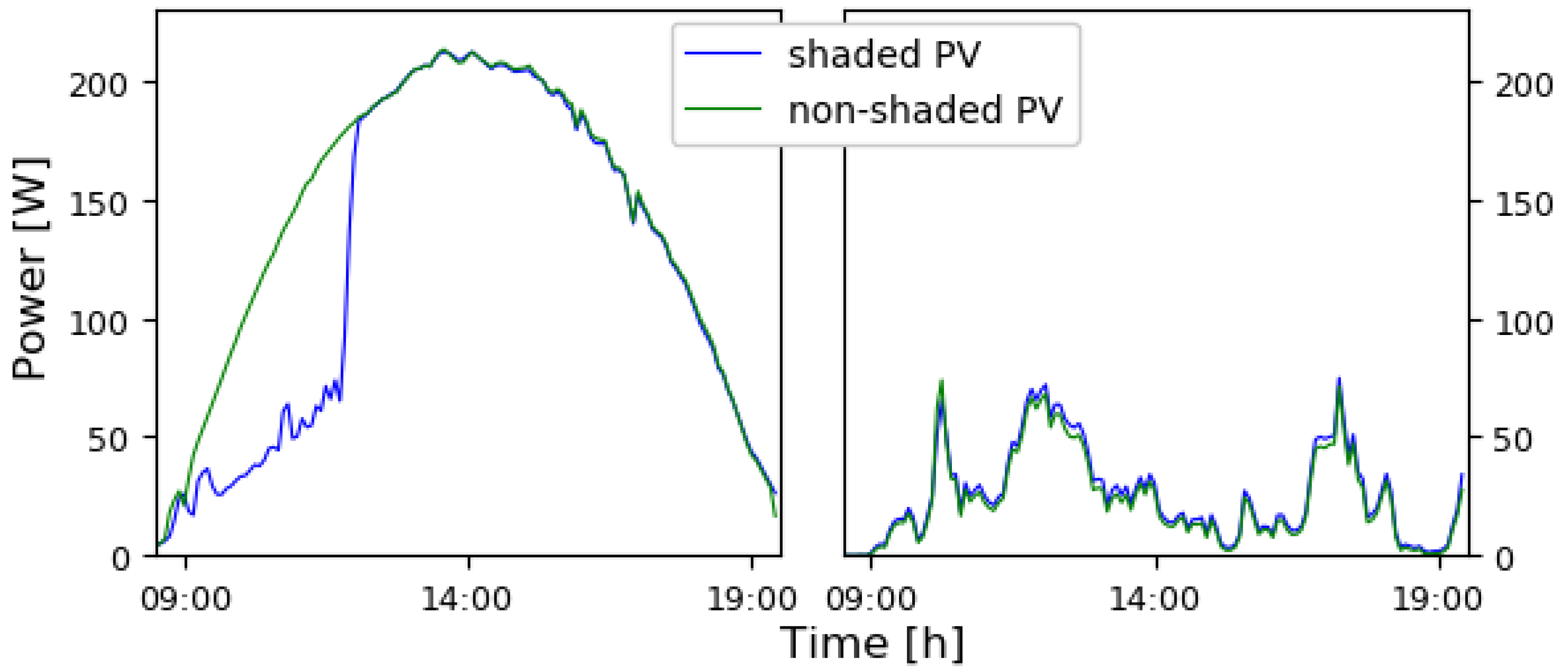
4.1. Example 1: Different Shadows on a Panel with Power Optimizer

In this example the application of the proposed algorithm for a panel with power optimizer is described, which was shaded at different hours by different objects during the day. The panel, similar to the whole system was shaded by a pole during two different periods, from April 21 to May 6 and from August 8 to October 13. Since it is the middle panel of the PV-system (Figure 2), the shade of the pole affected it during the day. Additionally, it is strongly shaded after mid-September by an unknown object, early in the morning. Like the presented example in Section 3, as reference the unshaded panel of the system with the power optimizers with the higher energy production is used.

In Figure 10, the shadow story of this panel is presented and in Figure 10 the distribution of DHI to GHI ratio of the blue markers of Figure 10 is presented. The algorithm detected four different shadow profiles, two for each shadow. Furthermore, while the shadows coexist for a short period, from October 1 to October 12, from 10:50 to 11:10, the algorithm is able to detect them as separate shadow stories.

4.2. Example 2: Panel with Micro Inverter and Morning Shadow

The proposed algorithm is applied to the system of the testing facility with micro inverters. The studied panel is connected with a micro inverter and it is shaded in the morning, similar to the example presented in the Section 3 (Figure 7). In contrast to the previous examples, the AC power of the micro inverter is used. As a reference system, the AC power of the micro inverter with the higher performance is used.

This example is slightly different than the previous one, since the day vs time scatterplot after the end of step II is presented as well (Figure 11a), together with the final scatterplot (Figure 11b). The purpose of these plots is to demonstrate the importance and the influence of step III and step IV in the process. After the second step, besides the pole shadow (from 9:30 to 12:00), the algorithm wrongly detects a small construction of outliers (from unknown reason) as shadow profile early in the morning between 15 and 30 July. Clearly, since the cause of these outliers is unknown and their duration short, they should not be characterized as shadow. That mistake is corrected in step III by means of the DBSCAN procedure. The shadow profile is deleted as the number of days the shadow is occurring was very few.

Another key fact to remember from this example is the change of the start and end hours of the main shadow late in winter, similar to the example of the methodology (Figure 7).

In Figure 12, the ratio of DHI to GHI of the moments where expected shadow is not observed is presented. As with the previous examples, the ratio of the strong majority of the measurements is higher than 0.5, thus the DHI was the dominant irradiance and the shadow is not detected.

5. Conclusions

In this paper a new method for the identification of shading on PV systems is introduced, based on the following data characteristics:

• Only the power output is used, which is the most common timeseries data for a PV system.
• Static system data is not necessary if the reference and the studied PV system have the same capacity.

The proposed algorithm analyzes a scatterplot of the power production of a PV system compared to a reference. Outliers in such a scatterplot (red markers in Figure 3a) are identified using a previously published method [25]. The principle of the new method is to study whether the outliers are occurring in the same time periods for consecutive days, which allows them to be characterized as shadows. Judging by the presented examples, the new method is able to detect the presence of a pole in front of a test system from the first day of its appearance on the rooftop, and is able to isolate and characterize, as malfunctions, other shadows from objects that are present at the rooftop for short periods (crane for rooftop maintenance, mid-June, Figure 7, Figure 10a and Figure 11b)

The algorithm is developed and tested on systems with module-level power electronics (MLPE), since these are quite popular in residential PV systems in the Netherlands, due to their effectiveness under shading conditions [28]. Furthermore, in MLPE systems, an unshaded panel can be used as a reference for the detection of the shadow in the rest of the panels and as stated in a previous survey, monitoring through neighboring panels of MLPE systems is more accurate than a pyranometer [25].

The proposed algorithm can be directly used in MLPE systems in its current form. However, its effectiveness on system-level power electronics system (PV system with string inverter) should be further examined before the method could be commercially used.

References

1. InterSolarEurope. Global Market Outlook For Solar Power/2018–2022; InterSolarEurope: Amsterdam, The Netherlands, 2018; p. 81. [Google Scholar]
2. SolarSolutions. Dutch Solar Trend Report 2018. 2018. Available online: http://www.solarsolutions.nl/download/ (accessed on 6 May 2019).
3. Centraal Bureau voor de Statistiek (CBS). Bijgeplaatst Vermogen Zonnestroom Bijgesteld n.d. Available online: https://www.cbs.nl/nl-nl/achtergrond/2015/51/bijgeplaatst-vermogen-zonnestroom-bijgesteld (accessed on 23 April 2019).
4. Solar Solutions Int. Nationaal Solar Trendrapport 2019; Solar Solutions Int: Amsterdam, The Netherlands, 2019. [Google Scholar]
5. EU. Directive 2010/31/ of the European Parliament on the Energy Performance of Buildings; EU: Brussels, Belgium, 2010; Volume 63. [Google Scholar]
6. Li, D.; Liu, G.; Liao, S. Solar potential in urban residential buildings. Sol. Energy 2015, 111, 225–235. [Google Scholar] [CrossRef]
7. Moraitis, P.; Kausika, B.; Nortier, N.; van Sark, W. Urban Environment and Solar PV Performance: The Case of the Netherlands. Energies 2018, 11, 1333. [Google Scholar] [CrossRef]
8. Woyte, A.; Richter, M.; Moser, D.; Green, M.; Mau, S.; Beyer, H.G. Analytical Monitoring of Grid-Connected Photovoltaic Systems; Technical Report IEA-PVPS T13-03:2014; IEA-PVPS: St. Ursen, Switcherland, 2014. [Google Scholar]
9. CENELEC IEC 61724. Photovoltaic System Performance Monitoring—Guidelines for Measurement, Data Exchange and Analysis; Edition 1.0, 1998-04; CENELEC IEC: Brussels, Belgium, 1998. [Google Scholar]
10. Ransome, S.; Wohlgemuth, J.H.; Poropat, S.; Aguilar, E. Advanced analysis of pv system performance using normalised measurement data. In Proceedings of the 31st IEEE PVSC, Orlando, FL, USA, 3–7 January 2005. [Google Scholar]
11. Van Sark, W.; Drews, A.; Heinemann, D.; Heilscher, G. PVSAT-2: Results of Field Test of the Satellite-Based PV System Perfomance. In Proceedings of the 21st European Photovoltaic Solar Energy Conference, Dresden, Germany, 4–8 September 2006; pp. 2–7. [Google Scholar]
12. Drews, A.; de Keizer, A.C.; Beyer, H.G.; Lorenz, E.; Betcke, J.; van Sark, W.G.J.H.M.; Heydenreich, W.; Wiemken, E.; Stettler, S.; Toggweiler, P.; et al. Monitoring and remote failure detection of grid-connected PV systems based on satellite observations. Sol. Energy 2007, 81, 548–564. [Google Scholar] [CrossRef] [Green Version]
13. Firth, S.K.; Lomas, K.J.; Rees, S.J. A simple model of PV system performance and its use in fault detection. Sol. Energy 2010, 84, 624–635. [Google Scholar] [CrossRef] [Green Version]
14. Chouder, A.; Silvestre, S. Automatic supervision and fault detection of PV systems based on power losses analysis. Energy Convers. Manag. 2010, 51, 1929–1937. [Google Scholar] [CrossRef]
15. Silvestre, S.; Chouder, A.; Karatepe, E. Automatic fault detection in grid connected PV systems. Sol. Energy 2013, 94, 119–127. [Google Scholar] [CrossRef]
16. Chouder, A.; Silvestre, S.; Sadaoui, N.; Rahmani, L. Simulation Modelling Practice and Theory Modeling and simulation of a grid connected PV system based on the evaluation of main PV module parameters. Simul. Model. Pract. Theory 2012, 20, 46–58. [Google Scholar] [CrossRef]
17. Eke, R.; Senturk, A. Monitoring the performance of single and triple junction amorphous silicon modules in two building integrated photovoltaic (BIPV) installations. Appl. Energy 2013, 109, 154–162. [Google Scholar] [CrossRef]
18. Chine, W.; Mellit, A.; Pavan, A.M.; Kalogirou, S.A. Fault detection method for grid-connected photovoltaic plants. Renew. Energy 2014, 66, 99–110. [Google Scholar] [CrossRef]
19. Jahn, U.; Farnung, B. Task 13—Performance and Reliability of PV Systems. Photovolt Power Syst Program Annu Rep 2016. 2017, p. 26. Available online: http://www.iea-pvps.org/index.php?id=57 (accessed on 6 May 2019).
20. Akram, M.N.; Lotfifard, S. Modeling and Health Monitoring of DC Side of Photovoltaic Array. IEEE Trans. Sustain. Energy 2015, 6, 1245–1253. [Google Scholar] [CrossRef]
21. Platon, R.; Martel, J.; Woodruff, N.; Chau, T.Y. Online Fault Detection in PV Systems. IEEE Trans. Sustain. Energy 2015, 6, 1200–1207. [Google Scholar] [CrossRef]
22. Dhimish, M.; Holmes, V. Fault detection algorithm for grid-connected photovoltaic plants. Sol. Energy 2016, 137, 236–245. [Google Scholar] [CrossRef]
23. Serrano-Luján, L.; Cadenas, J.M.; Faxas-Guzmán, J.; Urbina, A. Case of study: Photovoltaic faults recognition method based on data mining techniques. J. Renew. Sustain. Energy 2016, 8, 043506. [Google Scholar] [CrossRef]
24. Mallor, F.; León, T.; De Boeck, L.; Van Gulck, S.; Meulders, M.; Van Der Meerssche, B. A method for detecting malfunctions in PV solar panels based on electricity production monitoring. Sol. Energy 2017, 153, 51–63. [Google Scholar] [CrossRef]
25. Tsafarakis, O.; Sinapis, K.; van Sark, W.G.J.H.M. PV System Performance Evaluation by Clustering Production Data to Normal and Non-Normal Operation. Energies 2018, 11, 977. [Google Scholar] [CrossRef]
26. Libra, M.; Daneček, M.; Lešetický, J.; Poulek, V.; Sedláček, J.; Beránek, V. Monitoring of Defects of a Photovoltaic Power Plant Using a Drone. Energies 2019, 12, 795. [Google Scholar] [CrossRef]
27. Mohammedi, A.; Mezzai, N.; Rekioua, D.; Rekioua, T. Impact of shadow on the performances of a domestic photovoltaic pumping system incorporating an MPPT control: A case study in Bejaia, North Algeria. Energy Convers. Manag. 2014, 84, 20–29. [Google Scholar] [CrossRef]
28. Sinapis, K.; Litjens, G.; Van Den Donker, M.; Folkerts, W.; Van Sark, W. Outdoor characterization and comparison of string and MLPE under clear and partially shaded conditions. Energy Sci. Eng. 2015, 3, 510–519. [Google Scholar] [CrossRef] [Green Version]
29. Sinapis, K.; Tzikas, C.; Litjens, G.; Van Den Donker, M.; Folkerts, W.; Van Sark, W.G.J.H.M.; Smets, A. A comprehensive study on partial shading response of c-Si modules and yield modeling of string inverter and module level power electronics. Sol. Energy 2016, 135, 731–741. [Google Scholar] [CrossRef]
30. Topić, D.; Knežević, G.; Fekete, K. The mathematical model for finding an optimal PV system configuration for the given installation area providing a maximal lifetime profit. Sol. Energy 2017, 144, 750–757. [Google Scholar] [CrossRef]
31. Bressan, M.; El Basri, Y.; Galeano, A.G.; Alonso, C. A shadow fault detection method based on the standard error analysis of I-V curves. Renew. Energy 2016, 99, 1181–1190. [Google Scholar] [CrossRef]
32. Garoudja, E.; Harrou, F.; Sun, Y.; Kara, K.; Chouder, A.; Silvestre, S. Statistical fault detection in photovoltaic systems. Sol. Energy 2017, 150, 485–499. [Google Scholar] [CrossRef]
33. Bognár Loonen, R.C.G.M.; Valckenborg, R.M.E.; Hensen, J.L.M. An unsupervised method for identifying local PV shading based on AC power and regional irradiance data. Sol. Energy 2018, 174, 1068–1077. [Google Scholar] [CrossRef]
34. Lingfors, D.; Killinger, S.; Engerer, N.A.; Widén, J.; Bright, J.M. Identification of PV system shading using a LiDAR-based solar resource assessment model: An evaluation and cross-validation. Sol. Energy 2018, 159, 157–172. [Google Scholar] [CrossRef]
35. Libra, M.; Beránek, V.; Sedláček, J.; Poulek, V.; Tyukhov, I.I. Roof photovoltaic power plant operation during the solar eclipse. Sol. Energy 2016, 140, 109–112. [Google Scholar] [CrossRef]
36. Ester, M.; Kriegel, H.P.; Sander, J.; Xu, X. A Density-Based Algorithm for Discovering Clusters in Large Spatial Databases with Noise. In Proceedings of the Second International Conference on Knowledge Discovery and Data Mining, Portland, OR, USA, 2–4 August 1996; pp. 226–231. [Google Scholar]
Figure 1. Example of the effect of high direct irradiance (left plot) and high diffuse irradiance (right plot) on the shadow. The production of two similar panels with the same micro inverters is compared. The blue line represents the shaded panel, the green one the non-shaded panel. For clear sky conditions (left plot) the obstacle shadows the system, as evidenced by reduced power, while for a cloudy sky (right plot) the obstacle does not lead to reduced power.
Energies 12 01722 g001
Figure 2. The experimental facility of SEAC.
Energies 12 01722 g002
Figure 3. The data are clustered into inliers (green) and outliers (red), according to the algorithm [25]. (a) Scatterplot of studied panel vs the reference; (b) the green and red marked data points of (a) are plotted based on the date and time that they occur. Instead of power of the panels, their system yield is used, according to Equation (1).
Energies 12 01722 g003
Figure 4. The time distribution of the outliers of Figure 3. The shadow profile is detected to occur between 9:00 and 12:20, where the presence of outliers (red line) is stronger from both the inliers (green line) and the average presence of the outliers during the day. The fact that inliers are detected as well during these hours is due to days of high diffuse irradiance.
Energies 12 01722 g004
Figure 5. The plots of Figure 3 after the application of step II. The time limits of the shadows detected during step II (Figure 4) are applied in (b), where every fault within these time limits is characterized as shadow (black dots) and outside as malfunction (red dots). In blue colored the moments at which shadow is expected but did not appear, probably due to diffuse irradiance. In subfigure (a) the scatterplot of studied panel vs the reference with the new characterization is presented.
Energies 12 01722 g005
Figure 6. Application of DBSCAN for the derivation of the shadow profile to smaller groups. The marks, named as shadows in (a) are representing the different shaded days that DBSCAN assigns to different groups; three in the presented example. In (b), the final plot after the application of step III is presented.
Energies 12 01722 g006
Figure 7. Final plots of the shadow story. (a) Plot of studied PV vs reference PV, showing fewer blue markers compared to Figure 5a; (b) zoomed-in of (a); (c) periods with high concentration of outliers are characterized as shadows (black markers), and periods with low concentration of outliers as malfunctions (red markers).
Energies 12 01722 g007
Figure 8. The flowchart of the process.
Energies 12 01722 g008
Figure 9. The ratio of DHI to GHI for the blue markers in Figure 7. Clearly, for the strong majority of the measurements where shadow is expected but not observed, the DHI is the dominant irradiance.
Energies 12 01722 g009
Figure 10. The shadow story (a) of the middle front panel of the PV system with power optimizers. In contrast to the example in Section 3 (Figure 7), this panel is shaded by the pole around noon hours and by the short wall in-front of the system during early morning hours. Similar to Figure 7, many inliers are observed during the shadow profiles, but these are due to the high diffuse irradiance, as proven in (b).
Energies 12 01722 g010
Figure 11. The shadow story of panel with micro inverter, which similar with the example of the methodology (Figure 7) is shaded in the morning. In this case, the algorithm wrongly detects a shadow during step 2 (a). However, through steps 3 & 4 the algorithm auto-corrects the mistake and no extra shadow is presented in the final result, at subplot (b).
Energies 12 01722 g011
Figure 12. The ratio of DHI to GHI of the blue markers of Figure 11b.
Energies 12 01722 g012