Performance Prediction and Validation of a Small-Capacity Twisted Savonius Wind Turbine

Abstract

In this study, an off-grid–type small wind turbine for street lighting was designed and analyzed. Its performance was predicted using a computational fluid dynamics model. The proposed wind turbine has two blades with a radius of 0.29 m and a height of 1.30 m. Ansys Fluent, a commercial computational fluid dynamics solver, was used to predict the performance, and the k-omega SST model was used as the turbulence model. The simulation result revealed a tip-speed ratio of 0.54 with a maximum power coefficient, or an aerodynamic rotor efficiency of 0.17. A wind turbine was installed at a measurement site to validate the simulation, and a performance test was used to measure the power production. To compare the simulation results obtained from the CFD simulation with the measured electrical power performance, the efficiencies of the generator and the controller were measured using a motor-generator testbed. Also, the control strategy of the controller was found from the field test and applied to the simulation results. Comparing the results of the numerical simulation with the experiment, the maximum power-production error at the same wind speed was found to be 4.32%.

1. Introduction

The cumulative installation capacity of small wind turbines achieved 1.7 gigawatts (GW) in 2017 and is expected to reach 2.0 GW by 2020 [1,2,3,4,5]. Small wind turbines are defined slightly differently for different countries and standards; however, in Korea, they are classified as wind turbines with a rotor area smaller than 200 square meters, and a rated voltage lower than 1000 volts alternating current (VAC) or 1500 volts direct current (DC) [6].

Unlike utility-scale wind turbines, which have a rated power of 750 kW or higher, small-capacity wind turbines include various different types, e.g., horizontal axis or vertical axis and lift-type or drag-type [7]. Horizontal-axis wind turbines have higher aerodynamic efficiencies than their vertical-axis counterparts, and lift-type wind turbines have higher aerodynamic efficiencies than their drag-type counterparts. However, because small-capacity wind turbines are often installed in the vicinity of residential areas, other parameters, e.g., rotating speed, durability, noise, and visual impact, are often considered to be more important than efficiency. This is why drag-type wind turbines still survive and are used to generate electricity.

Drag-type wind turbines come in two varieties. One is the original Savonius wind turbine. The other is a modified version to increase its aerodynamic efficiency, which is called a twisted (or helical) Savonius wind turbine. Drag-type wind turbines used for electricity generation are mostly twisted Savonius wind turbines, due to their higher aerodynamic efficiency compared to the original Savonius wind turbines. Twisted Savonius wind turbines are commonly used to power street lamps with solar panels and small batteries. In most cases, these micro-wind turbines are installed at a street side as a cluster with more than two turbines. Based on recent studies, the energy efficiency of the micro-wind turbine cluster is found to be improved by optimized decision-making for turbine installation locations [8,9].

The blade-element momentum theory is used to analyze the performance of typical horizontal-axis wind turbines with two or three blades. The theory has been implemented in programs such as Bladed [10] and FAST [11], which are officially used by wind-turbine certification companies to verify the overall system performance. The theory has been experimentally validated over a long time and is now considered relatively accurate.

Two methods are typically used to analyze the aerodynamic performance of vertical-axis wind turbines. One is the single or multiple streamtube method [12,13]. These methods are implemented in programs, e.g., Qblade [14] and HAWC2 [15], and are used to analyze lift-type wind turbines, e.g., Darrious or H-Darrious wind turbines. The other method includes the RANS (Reynolds-averaged Navier–Stokes equations) or LES (Large Eddy Simulations) methods, which are implemented in general CFD (computational fluid dynamics) programs, e.g., Fluent or Ansys-CFX. Although simulation methods for horizontal-axis wind turbines have been thoroughly verified experimentally because they are the standard technology for utility-scale wind turbines, simulation methods and experimental validations for vertical-axis wind turbines are still limited. Furthermore, performance simulations and experimental validations for drag-type vertical-axis wind turbines are very rare.

The drag-type wind turbine, which is the subject of this study, rotates and generates electricity by the drag forces acting on the blade-surface sections. Thus, the shape of the turbine rotor affects the turbine performance. Therefore, selecting an optimized shape is crucial for wind-turbine performance. In the literature, optimum turbine-shape parameters for Savonius rotors have been suggested by researchers. Various studies present optimum values for the wind-turbine blade gap and the aspect ratio, defined as the blade height divided by the blade radius [16,17,18,19,20]. Blackwell [21] and Mahmoud [22] conducted studies on the blade number for optimal performance. Therefore, the wind turbine developed in this study was designed using the optimal parameters presented in the aforementioned literature.

As mentioned above, Savonius wind turbines rotate from the drag force on the blade sections. However, most commercial software for analyzing and designing wind turbines is limited to lift-type wind turbines that rotate by lift force. Therefore, many researchers have been analyzing Savonius wind turbines using general CFD software. Fujisawa [23] conducted a wind-turbine flow-field analysis and Modi [24] conducted a Savonius wind-turbine flow-field analysis by adapting the discrete vortex method. The power performance of the wind turbines was not presented in their studies.

Shinohara and Ishimatsu analyzed the performance of a Savonius-type wind turbine through CFD simulation [25]. Redchyts and Prykhodko also conducted a wind-turbine analysis using the unstructured finite-volume method [26].

Although most of the studies have carried out wind-turbine performance prediction by simulating the turbine-wake effect, etc., the experimental verification of simulation results using field tests is very rare. Therefore, in this study, an ultra-small wind turbine for urban street lighting was designed, based on the results in the literature, and its aerodynamic performance was predicted using CFD simulations. Based on the simulation results, a torque schedule for maximizing the aerodynamic efficiency was also proposed, and was implemented in the controller of a wind turbine. Finally, the wind-turbine performance predicted by simulation was verified by field tests. In addition, the performance test of the generator and controller assembly was conducted to obtain the efficiency of the power train of the wind turbine with respect to the rotational speed. Through the result of the test, the mechanical power of the rotor could be converted into electrical power and compared with the measured electrical power from the field test for experimental validation.

2. Simulation Modeling of a Wind Turbine

Figure 1 shows the simulation procedure to estimate the turbine performance. As the first step, a modeling was performed by smoothing sharp edges, eliminating unnecessary components including the generator, and generating meshes with suitable partitions. In this study, tetrahedral mesh was used for simulation. As the second step, the solution of the flow field was obtained. A pressure based transient method was used for the simulation, and the pressure and velocity distributions around the rotor were obtained. Finally as the third step, the rotor torque was obtained from the pressure distribution, and finally the mechanical power of the rotor was obtained based on the rotational speed of the rotor. The entire procedure from step 2 to step 3 was repeated with different rotational speeds to obtain simulations with different tip speed ratios.

2.1. Wind-Turbine Numerical Model and Parameters

The target wind turbine in this study is a drag-type twisted Savonius wind turbine with 2 blades. As shown in Figure 2 and

Table 1. Wind-turbine specifications.

Subject	Unit	Specification
Rotor Diameter	m	0.58 with 0.15 gap
Rotor Height	m	1.30
Turbine Type	-	Twisted Savonius

, the rotor of the target Savonius wind turbine is composed of two semi-circular blades with a diameter of 0.58 m and a height of 1.3 m. It has a gap of 0.15 m between the two blades so that air can pass through the gap. This type of air gap is shown in the literature to slightly increase the aerodynamic efficiency of the Savonius rotor. The mechanical power extracted by the rotor is converted into electrical power via a permanent-magnet synchronous generator, and the generated electrical power is stored in a 24 VDC battery. As generated power is stored in a battery, a type of turbine grid-off or independent grid system, then the main purpose of the turbine is lighting LED street lamps.

For a wind turbine, the most important parameter representing its power-production ability is the power coefficient, ${\mathrm{C}}_{\mathrm{P}}$ [26]. It can be defined as the non-dimensional ratio of the rotor’s mechanical power to the power carried by the wind passing through the rotor-swept area. The power coefficient is also known as the aerodynamic efficiency of the rotor, and can be calculated by

$$C_P=\frac{P_{\mathrm{mech}}}{0.5\rho A{V}^3}$$

(1)

where $P_{\mathrm{mech}}$ [W] is the mechanical power extracted by the rotor, $\rho$ [$\mathrm{kg}/{\mathrm{m}}^3$] is the air density, $A$ [${\mathrm{m}}^2$] is the rotor-swept area, and $V$ [m/s] is the wind speed.

Another variable that can explain the turbine’s characteristics is the tip-speed ratio. It is the ratio of the linear velocity at the blade tip to the wind speed [27], and is mathematically defined as

$$\mathsf{\lambda }=\frac{R\mathsf{\Omega }}{V}$$

(2)

where $R$ [m] is the radius of the wind turbine rotor, and $\mathsf{\Omega }$ [rad/s] is the rotational speed of the wind turbine rotor.

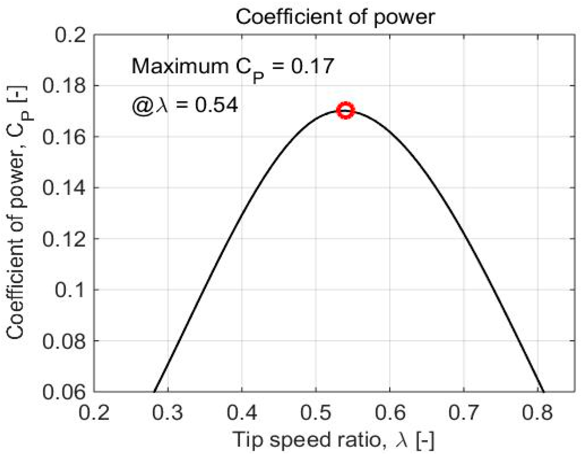
For all wind turbines, the power coefficient is a nonlinear function of the tip-speed ratio. It initially increases with the tip-speed ratio, reaches its maximum, and then decreases. Therefore, after the rotor is designed, it is essential to find out its maximum power coefficient and the tip-speed ratio where the maximum power coefficient is achieved. Then, this information is applied to the controller to maintain the optimum tip-speed ratio, regardless of the wind speed.

2.2. Computational Fluid Dynamics Model

To simulate the performance of the designed wind-turbine rotor, Ansys Fluent, a commercial computational fluid dynamics solver, was used, with a $k-\omega$ shear stress transport (SST) turbulent model. All the walls except the inlet, outlet, and rotor surface were set as non-slip walls. For the initial and boundary conditions, the wind speed was given at the inlet area, and the pressure-release condition at the outlet was used.

To conduct and calculate the rotor mechanical power produced by the blade rotation, a simulation was conducted with initial conditions, including the inlet speed, outlet pressure, and rotor rotational speed, in rpm.

For the simulation, the analysis domain is divided into four sections that are the upstream section, the internal section, the rotor, and the downstream section as shown in Figure 3a. The rotor is a solid geometry section. After the simulation, the rotor torque is calculated from this section’s area that contacts the internal section. This internal section rotates at the same speed as the rotor section and is the shape of a cylinder, including an entire rotor dimension of $\varphi 0.6\mathrm{m}\times \mathrm{h}1.30 \mathrm{m}$. This internal section is where the air particles flow around the rotor and causes rotor torque; hence, the rotor torque can be obtained in this section from the relation between the forces generated by the air drag and lift, and the distance from the rotational axis of the rotor. The inter-sectional area, with the rotor part and the boundary area similar to a wind tunnel, contains layered meshes that can help transfer the flowing particles’ momentum. The internal section is sandwiched by upstream and downstream sections. These sections have a 6-m width, 3-m height, and 5-m length. The length of the sections is about 10 rotor diameters (D).

With a divided fluid field and target bodies, a mesh was generated for a turbine analysis in the shape of a triangular pyramid, called a “Tetra” in Fluent and other solver tools. To prevent the analysis time delay and the convergence error caused by the mesh densification around complex and sharp elements, e.g., nuts and bolts, the frames are simplified or suppressed within a range that does not affect the aerodynamic performance and analysis. The element distribution and shape are shown in Figure 3b. The meshed model consists of 5,539,770 elements and 1,032,475 nodes.

To perform the flow analysis, the initial conditions for the velocity inlet and pressure outlet were defined as the wind speed and zero Pascals in gauge pressure, respectively. For the velocity inlet, the input wind speed was selected in the range of 3 m/s to 15 m/s with intervals of 2 m/s, and the rotational speed of the rotor was selected in the range of 10 rpm to 250 rpm. Considering the analysis time, the interval defining the rotational speed was selected as 30 rpm. The final output is the force and pressure acting on the rotor surface generated by the airflow and the torque calculated in the rotational axis to calculate the mechanical power. The analysis was performed at 0.01-s intervals, with 10-s for case.

3. Simulation Results

3.1. Pressure and Velocity Distribution

Figure 4 shows the CFD simulation results. Because of the tetrahedral mesh, the wind flow could not be aligned to the grid. In this case, the 2nd order accuracy method is known to be more accurate than the 1st order method. So, the level of the solution’s convergence and the accuracy of simulation was carried out using the 2nd order accuracy method. The rotor shown in the figure is in a state of rotation with a speed of 200 RPM under the mean wind speed of 13 m/s. Figure 4a shows the pressure distribution on the rotor surface and the surrounding area around the rotor. Based on the figure, the maximum pressure can be found to occur on the inner (concave) surface of the rotor that directly faces the incoming wind. At the same time, it can be seen that the direction of rotor rotation is counter-clockwise as the lowest pressure is distributed on the opposite outer (convex) surface. Figure 4b shows the velocity of air predicted under the same condition as Figure 4a. As the pressure of the fluid increases, the flow velocity decreases, resulting in the lowest value inside the rotor and the maximum value on the outer surface.

3.2. Power Coefficient vs. Tip-Speed Ratio

Based on the simulation model described in 2.2, a wind turbine performance prediction simulation was performed and the power coefficients were obtained with various operating conditions as shown in Figure 5. The horizontal axis of the figure is the tip speed ratio mentioned in Equation (2). As expected, the power coefficient increased nonlinearly as the tip speed increased and reached its maximum and decreased. According to the analysis, the maximum efficiency of the Savonius rotor was found to be 0.17 (17%) and the optimum tip speed ratio of the turbine was predicted to be 0.54. The power coefficients of other Savonius wind turbines available in the literature are found to be between 0.12 and 0.22 with the tip speed ratio between 0.4 and 0.6 [28,29]. Therefore the performance of the twisted Savonius wind turbine in this study is not much different from the performances of other twisted Savonius wind turbines with different capacities in the literature.

3.3. Power Curve Based on Maximum Power Coefficient

Figure 6 shows the aerodynamic power and the rotor speed with respect to the wind speed calculated with the assumption that the rotor speed is controlled to maintain the optimal tip speed ratio to achieve the maximum power coefficient as shown in Figure 5. The aerodynamic power in Figure 6a was calculated using Equation (1). The power coefficient used in the equation was 0.17, and the optimum tip speed ratio was 0.54. However, actual wind turbines need to consider external environmental conditions, such as electrical losses and overspeed protection, which may alter the torque-speed schedule of the generator and finally the turbine power performance. The power in Figure 5 does not reflect these external constraints and is just an ideal power production.

Figure 6b shows the rotational speed schedule calculated with the assumption that the maximum power point tracking (MPPT) control is performed with the optimum tip speed ratio of 0.54. Through the aforementioned Equation (2), the rotational speed can be calculated through the relationship of tip speed ratio and the wind speed. The result is a linear line shown in Figure 6b.

4. Power-Performance Test for Validation

For the verification and validation of the wind-turbine performance estimated by CFD simulation, the target twisted Savonius wind turbine was manufactured. Before the power performance testing of the wind turbine, a performance test of the generator was performed. Also, the power regulation scheme was determined and applied to the controller of the wind turbine.

4.1. Generator—Controller-related Test

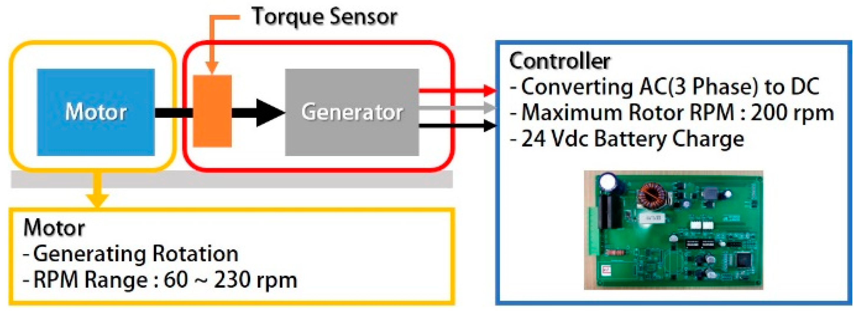
The performance test of the generator was conducted at Korea Test and Certification (KTC). As shown in Figure 7, the test facility consists of a motor that can simulate the mechanical power generated by a rotor, and a generator with a controller of the actual turbine system. The mechanical power generated by the motor is transferred to the generator through coupling, and the torque is measured through a torque sensor attached to the rotary shaft. The mechanical power, which is the input to the generator, the electrical power output from the generator (AC), and the power output from the controller (DC) are all obtained during the test. The test was carried out with 10 rpm intervals from 60 to 230 rpm, and the detailed test procedures with a schematic are as follows.

Firstly, the rotational speed of the motor is adjusted, and the mechanical power output is calculated through the rotational speed of the motor and the torque measured through the torque sensor. Also, the generator output is measured using a power analyzer. At this point, it is possible to calculate the generator efficiency by comparing it with the mechanical power. Finally, the output of the rectified power is analyzed through the controller and the efficiency of the controller is calculated by comparing it with the measured generator power.

Figure 8 shows the electrical efficiency of the generator and controller measured for various rotational speeds. The dots and circles are actual measured points and the dotted and dashed curves are their regression curves. The reason why the data have some scatters is that they include transients. Based on the figure, the generator efficiency (dashed line) increases slowly with the rotational speed of the generator. It is fluctuating but mostly lower than 0.7 when the rotational speed is lower than about 150 rpm, and becomes higher than 0.7 when the rotational speed is higher than 150 rpm. While the generator efficiency shows a relatively slow increasing trend, the controller efficiency (dashed line) significantly changes with the rotational speed. It starts with very low efficiency around 0.2 when the rotational speed is about 60 rpm and increases nonlinearly with the rotational speed. The efficiency reaches about 0.6 when the rotational speed is about 140 rpm, and after that an abrupt increase in efficiency is observed. Between 150 rpm and 190 rpm the efficiency of about 0.8 is maintained and after that it decreases to 0.74. Based on Figure 7, at least 130 rpm is needed to achieve the controller efficiency of 0.6.

4.2. Test Environments

The power-performance test of the wind turbine was carried out at the small wind-turbine test site of Kangwon National University, which is located at Pyeongchang, Gangwon Province, Korea. The average wind speed at the 10-m hub height was 4.6 m/s during the test.

The power performance test of a wind turbine consists of the power measurement of the wind turbine and the measurement of wind data. Wind data including wind speed and direction were measured through sensors installed to a mast at the hub height of the wind turbine. The mast was located about 4 rotor diameter (RD) away from the wind turbine. The wind speed was measured using an anemometer and an F–V Converter was used to convert the frequency obtained from the sensor to voltage. To measure the wind turbine power, a power analyzer was used. The generated power and the wind data were stored in a personal computer through a data acquisition system. All the data were saved with a 1 Hz sampling rate.

4.3. Measured Test Results

Figure 9 shows the measurement results of the wind turbine. Figure 9a shows the measured electrical power with respect to wind speed. The dots in the figure represent one-minute averaged power which is used to show the power performance of a small capacity wind turbine based on the standard. The solid line with asterisks in the figure represents the averaged value in a bin, which has an interval of 0.5 m/s. Figure 9b shows the rotational speed of the generator with respect to the wind speed. The rotational speed of the generator was calculated using,

$${\mathrm{N}}_{\mathrm{s}}=\frac{120f}{P}$$

(3)

In Equation (3), f is the frequency of a single-phase voltage signal, p is the number of the generator poles, and Ns is the rotational speed in revolutions per minute (RPM). The number of poles of the generator used for the Savonius wind turbine was 20. The dots in Figure 9b represent one-minute averaged values like the dots in Figure 9a.

4.4. Control

The result shown in Figure 10a is the change in the tip speed ratio as the wind speed increases. The tip speed ratio values of the one minute averaged data were obtained using Equation (2) with the measured rotational speed of the generator in Figure 9b. Based on the figure, the tip speed ratio was high when the wind speed was small and decreased nonlinearly. When the wind speed was between 7.5 m/s and 9 m/s, the tip speed ratio was about 0.57, which is the optimal tip speed ratio to achieve the maximum power coefficient, 0.54. Also, the tip speed ratio decreased as the wind speed increased after 9 m/s. Based on Figure 10a, the control strategy of the controller can be obtained. When the wind speed is small, the generator torque values are lower than the optimum values to achieve the optimum tip speed ratio and as a result, the generator speed becomes higher and finally the tip speed ratio becomes higher. When the wind speed is high, the generator torque values are higher than the optimum values to achieve the optimum tip speed ratio and as the result, the generator speed becomes lower and finally the tip speed ratio becomes smaller. This control strategy is suitable to avoid the low efficiency region based on the efficiency characteristic of the controller shown in Figure 8 when the wind speed is low, and also to protect the system by preventing overspeed of the generator.

Figure 10b shows the power coefficient calculated from the simulation data in Figure 4 with the tip speed ratios obtained from the test data in Figure 10a. It is clearly shown in the figure that the power coefficient decreases as the tip speed ratio deviates from the optimal value.

Figure 11 shows the aerodynamic power with the maximum power point tracking strategy obtained from the simulation (dashed line), and the aerodynamic power calculated with the tip speed ratios obtained from the test results in Figure 10a (solid line). Due to the algorithm in the controller, it can be found that the aerodynamic power of the rotor slightly deviates when the wind speed is lower than about 7 m/s or higher than about 9 m/s.

5. Discussion

Figure 12 shows a comparison of the measured wind turbine output with the simulation results. The solid line with squares shown in the figure represent the measured wind turbine power converted to Bin data. The curve with circles shows the predicted power performance of wind turbines through simulation. To compare errors with simulation results, a ± 10% error range is described by error bars, and the data interval for simulation was chosen as 0.5 m/s. The simulation results in Figure 12 include both the efficiency of the generator and the controller with respect to the rotor speed in Figure 8 and the power coefficient based on the torque schedule of the wind turbine in Figure 9b. The comparison shows that the two data have the same increasing trend, and the maximum prediction error is found to be about 4.32% (@12m/s) within the measured and predicted ranges.

6. Conclusions

In this study, a drag-type Savonious wind turbine rotor with a diameter of 0.58 m and a height of 1.32 m was designed and tested. The rotor was modelled in a commercial CFD program and its aerodynamic performance was predicted through simulations. The simulation confirmed that the maximum power coefficient of wind turbines is 0.17 at a tip speed ratio of 0.54. Based on this, the power curve with the maximum power point tracking was obtained.

The simulation results were compared with test results of the designed wind turbine with a generator and a controller. For comparisons, the aerodynamic power was obtained with tip speed ratio data from the field test based on the control strategy imbedded into the controller of the wind turbine. Also the electrical conversion efficiencies of the generator and the controller were found from a motor-generator test and considered for the comparison. From the comparison, the simulation results were validated with a maximum error of 4.32% in power estimation at 12 m/s.