Abstract
Globalization has led to an increase in the use of small copters for different activities such as geo-referencing, agricultural fields monitoring, survillance, among others. This is the main reason why there is a strong interest in the performance of small-scale propellers used in unmanned aerial vehicles. The flow developed by rotors is complex and the estimation of its aerodynamic performance is not a trivial process. In addition, viscous effects, when the rotor operates at low Reynolds, affect its performance. In the present paper, two different computational methods, Computational Fluid Dynamics (CFD) and the Unsteady Vortex Lattice Method (UVLM) with a viscous correction, were used to study the performance of an isolated rotor of a quadcopter flying at hover. The Multi Reference Frame model and transition turbulence model were used in the CFD simulations. The tip vortex core growth was used to account for the viscous effects in the UVLM. The wake structure, pressure coefficient, thrust and torque predictions from both methods are compared. Thrust and torque results from simulations were validated by means of experimental results of a characterization of a single rotor. Finally, figure of merit of the rotor is evaluated showing that UVLM overestimates the efficiency of the rotor; meanwhile, CFD predictions are close to experimental values.
1. Introduction
Unmanned Aerial Vehicles (UAVs) is a growing technology developed to be used in different applications such as geo-referencing, agricultural monitoring and security among many others. Within platforms available to build UAVs, the quadcopter is one of the most used, as it is a Vertical Takeoff and Landing (VTOL) Vehicle, easy to maneuver and to control. The aerodynamic behavior of these vehicles depends on the efficiency of the rotors and, hence, its performance is strongly affected by the wake developed by a single rotor and its interaction with the other rotors and fuselage.
The study of the flow developed by the rotors is complex, however, different techniques have been applied to predict aerodynamic parameters of the rotors. Momentum theory and the blade element theory are theoretical approximations to estimate thrust () and power () coefficients, but these are based on strong fluid simplifications. Further refinements of these models were constructed based on empirical parameters obtained by experimental studies of rotors used in helicopters; therefore, the applicability of these data to study small rotors is not advisable. Nevertheless, these techniques can be employed as good preliminary approximations [1].
Different authors have studied the aerodynamics of the rotors through Computational Fluid Dynamics (CFD). Doerffer and Szulc [2] investigated the flow field near a hovering model of the Caradonna and Tung helicopter rotor, which is a test-case extensively used within the helicopter community for validation of CFD codes applied to rotorcraft problems. They used a compressible Reynolds-averaged Navier–Stokes (RANS) model based on the Spalart–Allmaras equation and a density based formulation. The flow field is quasi-steady respect to the blade and periodic in nature; therefore, only one blade was simulated. A structured mesh of 5.7 million cells with was used. They found an underestimation of of the prediction of the thrust coefficient, and a slight deviation of the load distribution along the span of the blade in comparison to experimental data was evident. However, RANS models are known to be extremely dissipative when using structured grids, a tip vortex age of approximately 450 was resolved.
Pandey et al. [3] conducted simulations to analyze the flow around an isolated main helicopter rotor at an angular velocity of 800 RPM, angle of attack of 8 and a blade profile of standard ONERA OA209 airfoil used in a Eurocopter AS350B3 helicopter (France) during hovering flight conditions. A RANS model with the turbulence model and multi-reference frame method (MRF) were used. From the vorticity field, two clear vortex zones at the tip of the blade and at the trailing edge were found that could affect the lift of the helicopter, resulting in unsteady hover and increased noise. An increase in the drag of the rotor disk section leading to energy losses was evident.
Gomez et al. [4] analyzed the effects that a bio-inspired rotor blade shape have on the size and structure of a tip vortex. Four different insect species were considered, but the cicada wing was selected to conduct CFD simulations. The computational domain was meshed with an unstructured grid of 2 million cells. The implicit unsteady model was used with the first-order temporal discretization. A second order discretization scheme was used with implicit integration using the algebraic multigrid (AMG) linear solver for all flow variables. The Menter’s Shear Stress Transport (SST) version of the turbulence model was used with curvature correction enabled. Vorticity magnitude contours showed smaller areas of high intensity for the vortex generated by the bio-inspired blade compared to the ones found when using a shed from a rectangular blade. Furthermore, the rectangular blade presents higher values of turbulent kinetic energy over a greater area than those for the bio-inspired blade. The peak of the axial velocity deficit in the vortex behind the bio-inspired blade was lower than the vortex generated by the rectangular blade. Finally, results demonstrated advantages of the bio-inspired blade, as the vortex size and strength is reduced at the tip of the blade.
Jiang and Zhang [5] studied the effect of the pitch angle, thickness, aspect ratio, number of blades, and radius of duct inlet lip of an annular lift fan aircraft during hovering. An unstructured tetrahedral volume mesh was used, the RANS model with a pressure-based solver, the Green–Gauss node based gradient option, steady approach and the (SST) turbulence model were applied. The semi implicit method for pressure linked equations (SIMPLE) scheme was used with the second order discretization for the pressure equation; the third order monotonic upstream-centered scheme for conservation laws (MUSCL) for the momentum, turbulent kinetic energy and turbulent dissipation rate were selected. The MRF model was used to analyze the fan fluid zone and the stationary zone. Validation of the numerical model was performed on a conventional circular lift fan employed in VTOL UAVs, resulting in good agreement with experimental values for the thrust and figure of merit (). Results showed that the highest FM values were obtained when using a pitch angle of 27, a thin blade with maximum thickness of of the chord length and a high aspect ratio between to . The number of blades affects the performance of the rotor in such a way that, for 32 blades, the highest value of FM was achieved, while the twist of blades deteriorates the performance and taper blades do not improve efficiency.
Duraisamy and Baeder [6] used a high-resolution RANS solver applied to study the evolution of tip vortices from rotary blades. Computations were performed using a modified version of the compressible RANS code TURNS. The inviscid terms were computed using the third/fifth order WENO (Weighted Essentially Non-Oscillatory) schemes. The viscous terms were computed using the second/fourth order central differencing. The Spalart–Allmaras turbulence model with rotational correction was used and the equations were solved in the rotating reference frame. A blade grid of approximately 4.9 million points and a refined overset grid of 2.9 million points were used to resolve the tip vortex; to account for the far-field boundaries, a cylindrical background mesh of 2.9 million points was utilized. Results of the simulations were compared with experimental data collected by Caradonna and Tung [7]. It is evident that the fine grid solution compares well with experimental measurements at all radial locations. The coarse grid solution is noticeably poor in the inboard stations, which is possibly a result of inadequate resolution in the spanwise direction. RANS simulation of tip vortex presents numerical diffusion, which arises primarily from inaccuracies in the discretization of the convective term in the Navier–Stokes equations and inaccurate turbulence modeling. A numerical diffusion error was reduced using proper grid resolution and high order numerical schemes. Reliable solutions can be obtained by adding a simple rotational correction to the production term in the Spalart–Allmaras turbulence model.
Potsdam and Pulliam [8] investigated the influence of turbulence modeling in vortical wake of rotorcraft simulations. They performed CFD simulations using the OVERFLOW RANS equations solver. The domain was meshed with a structured overset of grids using body conforming near-body grids (NB) and off-body grids (OB) in the wake far field. A modified source/sink boundary condition was implemented for hover, and both the steady and conventional moving grid unsteady formulations were used and compared. They found that a turbulence model, incorrectly sensitized to vorticity, performs poorly leading to excessive turbulence production in the vertical wake. In addition, the moving grid (unsteady formulation) gives better accuracy than those found for a steady state formulation in simulations of an isolated rotor in hover; the cause of this difference is not defined.
Yoon et al. [9] compared the effect of RANS and Laminar Off-Body models on the accuracy of solutions for rotor flows in hover. They used a 25 ft diameter XV-15 isolated rotor, which consists of three highly twisted rotor blades and a simplified hub. The approach consisted on an inertial coordinate system where near-body (NB) curvilinear O-grids rotate through a fixed off-body (OB) Cartesian grid system; 62 grids with a total of 47.2 million points were necessary to perform the simulations. The Pulliam–Chaussee diagonal central difference algorithm was used with 5th order spatial differencing. Dual time-stepping is used to advance the simulation in time with 2nd order time accuracy and the Detached Eddy Simulation (DES) based on the Spalart–Allmaras was used as turbulence model. The Laminar Off-Body (LOB) model is also used and it assumes that the turbulent eddy viscosity that is generated, e.g., on the rotor blades, can be convected, but not produced, dissipated, or diffused in the lower wake OB grids. The difference in the predicted FM between both models is less than with an LOB prediction slightly higher.
More recently, CFD has been applied in more complex simulations involving not only the aerodynamics of the rotor but also the specific application of the copter. Yang et al. [10] implemented a very complex CFD simulation in which a complete multicopter, which is typically used for plant protection, was simulated in hover flight close to the ground. The main purpose of this model was to simulate the interaction of the wake of the rotors with the droplets that are sprayed from the multicopter. Numerical results show very good agreement not only in the predicted velocities in the wake but also in the distribution of droplet size and spray width.
However, numerous authors have used CFD simulation to study the flow developed by a rotor at hover, and its application is limited because of its computational cost. Therefore, some researchers have been applying diverse approximations to study the aerodynamics of rotors. Some of these methods are known as time marching free vortex wakes such as the Unsteady Vortex Lattice Method (UVLM). Szymendera [11] implemented a free wake vortex lattice method to predict the wake structure and blade loading for a rotor in arbitrary motion by modeling the rotor blades as flat plates. A Prandtl–Glauert correction was applied to the Biot–Savart Law to model compressible flow. The code was validated using data from two experimental hover studies: the first, for incompressible flow and the second, for a compressible flow at the tip. Each simulation was ran for eight revolutions and the results were compared with experimental lift and pressure coefficients. Both versions (compressible and incompressible) produced similar results and closely match experimental data. Despite the fact that the compressible version slightly overpredicts the lift inboard the tip, it does predict an increased lift. It was concluded that applying the Prandtl–Glauert correction leads to severe overpredictions of the lift, i.e., this technique may be useful for fixed wings, but it is not valid to be used for rotating blades.
Shreyas [12] studied the wake developed by a rotor during maneuvering conditions using a free-vortex wake method. Besides the free vortex wake model, a flapping and the viscous core growth model was used. To solve the convection of the free vortex in the wake, a second order predictor corrector scheme was implemented. Results were validated using experimental data reported in the literature. This methodology showed a high flexibility and can be used to simulate the rotor wake and to predict its aerodynamics parameters at hover or during maneuvering. It was found that tip vortices try to pair up and bundle into a toroidal structure below the rotor, which are unstable and dissipate as they are convected downstream.
Colmenares, López and Preidikman [13] developed the GUAVLAM code based on UVLM to simulate the potential flow around a lifting surface. The code was tested by simulating two rectangular untwisted blades. Simulations were performed using rotors with two, three and four blades and for eight revolutions in each case. Results showed an interaction of the blades with the fuselage that leads to oscillations on the aerodynamic loads, but it was reduced as the number of blades increases. A major impact on the generation of thrust due to the number of blades was found, while the geometrical configuration had a minor influence.
To the best of the authors’ knowledge, the UVLM has not been used to study the aerodynamic performance of small rotors as the employed in the quadcopter ARAKNOS V2 from the Colombian company ADVECTOR (Chia, Cundinamarca) (see Figure 1). At low or moderate Reynolds, the viscous effects cannot be neglected; therefore, a viscous correction was implemented to the GUAVLAM code and then it is used to simulate the studied rotor. In addition, for the present research article, CFD simulations are performed using a commercial software to study the hover aerodynamic performance of the selected rotor. A comparison between results obtained by both methods is presented and validated with experimental data. Finally, a simple model to estimate the efficiency and flight time for hover missions of the ARAKNOS V2 quadcopter is proposed.
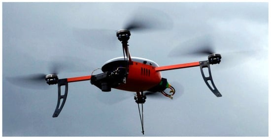
Figure 1.
Quadcopter ARAKNOS V2.
2. Computational Methodology
2.1. CFD Model
The simulations were performed in steady state using the Multi-Reference Frame (MRF) model, assuming incompressible flow for which the governing equations are:
Notice that Equations (1) and (2) are written in a non-inertial reference frame attached to the rotor, but the velocities are referenced to an inertial reference frame, so that is the absolute velocity (inertial reference frame), is the relative velocity, and is the rotational velocity of the non-inertial frame. In this case, Coriolis and centripetal accelerations are into a single term . By using this formulation, it is possible to achieve steady-state solutions when prescribing suitable boundary conditions and is constant. A transition turbulence model, based on the coupling of the SST transport equations with two additional equations, one for the intermittency and the other for the transition state, was used. Curvature correction option was also enabled. A detailed description of the turbulence model can be found in Refs. [14,15]. In this problem, the complete computational domain refers to a single rotating reference frame located at the center of the propeller. It is possible to find a steady state solution if is constant and the boundary conditions are well established.
All simulations were implemented in the CFD software ANSYS FLUENT v17.0 (ANSYS, Canonsburg, PA, USA). The pressure-velocity coupling scheme SIMPLE with least squares cell-based evaluation, for the gradients, was used. Second order upwind discretization was used for momentum equation convective terms, while first order upwind discretization for the convective terms were used for the turbulence model equations due to numerical stability problems. Regarding the diffusive terms, second order discretization was used in all the equations. Simulations were performed increasing the rotational velocity with small discrete steps: solutions for velocities from 1 RPM up to 64 RPM ( @ 64RPM = 1607 and Ma = 3.6 × ) were obtained assuming laminar flow and for velocities between 120 RPM and 6500 RPM ( @ 6500RPM = 1.632 × and ), the SST transition model was enabled. For each angular velocity, the simulation ran until residuals reached a convergence criteria of 1 × 10. The working fluid is air at the same conditions as in the experimental tests (see Section 3). Complete simulations (from 1 RPM up to 6500 RPM) took approximately 150,000 iterations.
CFD Computational Domain
The CAD model of the carbon fiber commercial rotor was obtained by means of 3D scanning technique (see Figure 2). The diameter of the rotor (DP) is 360 mm, root chord is mm, tip chord is mm and the chord length at of the span is mm.
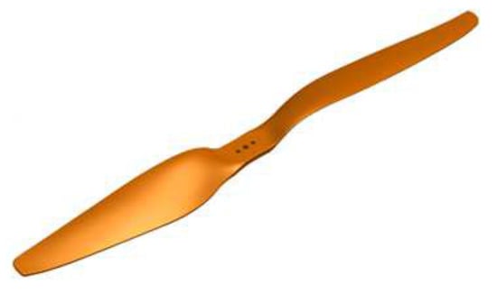
Figure 2.
ARAKNOS V2 Rotor CAD.
As shown in Figure 3, the computational domain is a cylinder, with a diameter of DP and 7DP in length; the propeller is centered in the domain and at DP from the upper surface. Boundary conditions were specified as follows: pressure inlet for the upper and lateral surfaces and pressure outlet for the lower surface, the intermittency was set as 0 and the turbulent intensity at 1%; the surface of the propeller was modeled as a non-slip wall.
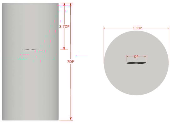
Figure 3.
Computational CFD domain.
The domain was meshed with an unstructured grid of tetrahedral elements and a refined grid of pyramidal elements near the propeller surface (see Figure 4). The quality of the mesh near the rotor surface guaranties a < 1. A convergence analysis was performed using six different grids and varying the number of elements from 0.8 to 16 million. Torque and thrust at 5221 RPM were chosen as convergence criteria. Figure 5 shows that an increase of the number of elements from 9.6 to 16.5 million leads to a difference in the predicted thrust of and for torque. Table 1 shows the parameters and quality characteristics for the meshes used in the grid convergence analysis. Orthogonal quality values close to 0 and skewness values close to 1 indicate low quality. It is clear that more than 70% of the elements have an orthogonal quality higher than 0.8 for meshes C, D and E. For meshes D and E, the skewness is lower that 0.3 for almost more than 60% of the elements. Despite that the quality of the mesh can be considered acceptable, a mesh with million elements was selected (Mesh E).
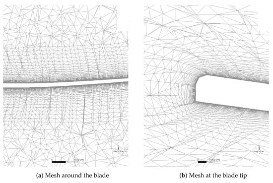
Figure 4.
Mesh.
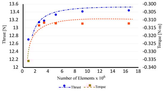
Figure 5.
Convergence study.

Table 1.
Mesh characteristics for the convergence study.
2.2. Unsteady Vortex Lattice Method
The Unsteady Vortex Lattice Method (UVLM) is a computational, low-order method used to solve incompressible, inviscid and irrotational flows around lifting surfaces, which are governed by the Laplace equation (Equation (3)).
Based on the superposition principle, the solution of the Laplace equation can be achieved by adding solutions of simple incompressible, inviscid and irrotational flows such as: sources, sinks, doublets and vortex lines or filaments. In UVLM, the lifting surfaces are considered thin such that the vorticity is confined in a very thin layer over them. In this case, the vorticity distribution is done with vortex filaments arranged in loops over the lifting surface. For potential flows composed only by vortex filaments, the Helmholtz theorems state:
- The circulation of a vortex filament () is constant along the filament,
- The vortex filament has to be a closed loop or extend to infinity,
- The flow is initially irrotational and will remain irrotational.
The velocity induced at any point , by a filament of vorticity with strength and length L, from point to point is calculated using the Biot–Savart law Equation (4) (see Figure 6):
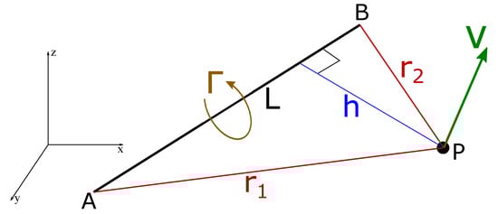
Figure 6.
Biot–Savart law formulation.
The lifting surface is discretized with quadrilateral panels, each panel has a control point at the geometrical center of the panel, and at each panel a vortex loop is located. The edges of these loops are filaments of finite vorticity. The UVLM estimates the circulations of each vorticity filament on the discretized surface, such that the normal velocity at the control points is zero (non-penetration condition). To enforce spatial conservation of circulation, it is assumed that each vortex loop has a constant circulation []; then, the circulation for each vortex filament is calculated as .
Filaments of vorticity induce a velocity at the control point of the panels; then, the sum of the induced velocities, the velocity of the lifting surface and the free-stream velocity must satisfy the non-penetration boundary condition at each control point as shown in Equation (5):
where the Left-Hand side of Equation (5) represents the velocity induced by the vortex sheet bounded to the surface. is the normal component of the velocity induced on panel i by panel j with unitary circulation, is the number of bound vortex sheet, is the velocity of the lifting surface at the control point i, is the velocity induced by the wake on panel i, is the free-stream velocity and is the unity vector normal to the surface at the panel i (see Figure 7).
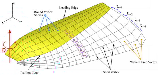
Figure 7.
Descriptive diagram of the Unsteady Vortex-Lattice Method (UVLM).
In order to satisfy the Kutta condition at each time step, the vortex loops of the trailing edge are shed to the wake tangentially, but their circulations remain constant. Lagrangian points of the wake move with the free-stream velocity and the induced velocity, by all surface and wake vortices (Equation (6)):
where is the position vector of any Lagrangian point of the wake, is its total velocity calculated through Equation (7) and t is the time. To solve Equation (6), a predictor–corrector scheme was implemented. For the predictor step, each vortex point position is calculated by means of Equation (8). The corrector step estimates a new velocity field based on the position of vortex points computed in the predictor step. With this new velocity, it is possible to calculate the final positions of the wake points using Equation (9):
2.2.1. UVLM Viscous Correction
The Varistas model [16] is used as the main vortex model in order to improve the results of the Biot–Savart law (Equation (4)) when . Then, the corrected Biot–Savart equation is given by Equation (10), where is the vortex core radius:
To incorporate the effects of the viscosity, the vortex core growth model was implemented. This model includes the viscous diffusion and has been developed from experimental studies which have shown that the vortex core radius varies with the square root of time [17] (see Equation (11))
where can be found from the Lamb–Oseen vortex model for the swirl velocity [18]. From experimental measurements, it is possible to conclude that the vortex core growth is higher than the calculated through Equation (11) due to turbulence vorticity diffusion (see Equation (12)):
where is the non-zero effective core radius at the tip vortex origin when the wake age is , is the viscosity, is the angular velocity, is the wake age and is an average “turbulent” viscosity coefficient. Measurement of the initial core radius of trailing vortices are typical of the order of the airfoil thickness at the wing tip [18]. The average turbulent viscosity coefficient is formulated in terms of the vortex Reynolds number
where is a parameter to be determined from experimental studies. Mahendra and Leishman [18] analyzed the results of diverse experimental studies and found that a value of best describes the physical nature of the vortex core growth. is the value that better approximates to the experimental results for small rotors as demonstrated in Ref. [18].
2.2.2. Forces and Torque Estimation
The pressure distribution and the pressure coefficient () are calculated by means of the unsteady Bernoulli equation applied to a velocity field:
The pressure jump at each control point is calculated using non-dimensional quantities (for details, see Ref. [13]); therefore, Equation (16) becomes Equation (17)
where is the non-dimensional mean velocity at the control point i, is the non-dimensional tangential velocity jump at panel i, and is the loop circulation at the panel.
From the pressure distribution, it is possible to calculate the acting force (Equation (18)) and moment (Equation (19)) coefficients [13]:
where is the non-dimensional area of panel i, and is the non-dimensional position vector of control point i from the center of rotation and the unity vector normal of the panel i. Finally, the thrust coefficient is obtained from the component of the acting force in the Z direction (i.e., ) (see Figure 7):
In the present study, the mean surface of the actual 3D scanned rotor was used as lifting surface. This surface was discretized using a total of () panels. A numerical study was performed in order to determine the influence of the number of panels in the predicted torque and thrust, but no significant effect was found. UVLM simulations were initialized by a slow-starting method beginning at a nearly 0 non-dimensional velocity and increased up to 1 in 40 linear steps. Details of the implementation of the slow-starting method can be found in Ref. [13]. After the slow-start phase, the simulations were run for at least eight revolutions with a time step that corresponds to a rotation of 10. Figure 8 shows the evolution of the thrust coefficient. It is clear that the first 40 time steps correspond to the slow-starting method, in which the value overshoots due to the unsteadiness of the flow. After this overshoot, decreases in magnitude for at least another revolution of the rotor. It is also observed that reached a steady value, after six more revolutions of the rotor. Final force and torque coefficient values were calculated as the average of their results for the last revolution.
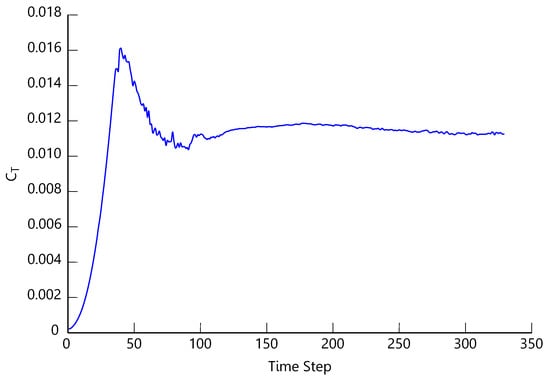
Figure 8.
Thrust coefficient evolution.
3. Experimental Methodology
Static tests were executed to characterize the performance of the rotor which is a carbon fiber propeller. A brushless motor of 530 RPM per volt (RCTimer Power Model Co., Ltd, HongKong), with a maximum power of W at 14.8 V and 11990 RPM as maximum rotational velocity without load is used [19]. The tests consisted on discrete increments of the angular velocity from 1500 RPM up to 6500 RPM. Each velocity step needed around 60 s to reach steady state, after that the angular velocity was increased. The velocity of the brushless motor is controlled by sending a Pulse Width Modulation (PWM) signal to the Electronic Speed Control (ESC) through a “Pololu Micro-Maestro” servo controller card. A “Keithley” (2260B-80-27 720W) voltage source is used as the DC (Direct Current) power supply set at 15 V. Pressure, temperature and relative humidity were measured in order to estimate the air density and viscosity.
Thrust and torque measurement were obtained by using a “RC Benchmark” commercial dynamometer 1580 series [20], which uses two (2) load cells to measure the torque and one (1) load cell to measure thrust. The device allows the user to check the frequency of the PWM signal to estimate the RPMs of the motor. Besides the estimated RPM, the angular velocity was measured by an optical photo-transistor Omron E3FB (OMROM, Japan). Its operational distance ranges between and m and a response time of ms. A Labview code was implemented to translate the output frequency into RPM. A schematic diagram of the experimental setup is shown in Figure 9.
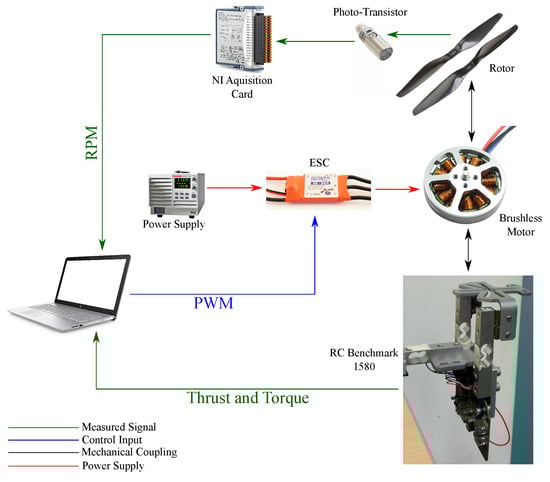
Figure 9.
Experimental setup.
Density of air is calculated using the model shown in reference [21] (Equation (21))
where is the molar mass of dry air, is the barometric pressure, Z is the compressibility factor, R is the molar gas constant, T is the temperature and is the mole fraction of water vapour. Z and are dependent on , T and (relative humidity). Pressure was measured with a Vaisala PTB330TS barometer (Vantaa, Finlandia), while the relative humidity and temperature were measured with an EXTECH 45158 anemometer (Waltham, MA, USA) (see Table 2). Viscosity was calculated using the Sutherland’s equation at atmospheric conditions of the test that are listed in Table 3.
Table 2.
Instrumentation characteristics.
Table 3.
Experimental air conditions.
Tests were performed at a not atmospheric controlled laboratory at the altitude of Bogota, Colombia. Each experimental test took approximately 15 min and all tests were performed on the same day. As the experiments were not long, only small variations of ambient pressure, humidity and temperature were observed and not taken under consideration. Pressure, temperature and relative humidity reported in Table 3 are the average of the measured values during the tests.
4. Results
Numerical results are organized in two groups: first, field variables’ results such as vorticity field and pressure distribution along the rotor surface are shown and discussed. Then, integral variables such as thrust, torque and figure of merit (FM) are estimated and compared with experimental data.
4.1. Wake Visualization
For CFD results, the Q criterion [22] is applied to visualize the wake generated by the rotor. It is important to mention that the visualized Q criterion field corresponds to one estimated from the vorticity field observed from the non-inertial reference frame. Figure 10a shows the wake generated at 4000 RPM while Figure 10b, the wake at 6000 RPM. It is clear that tip vortices are wider and, therefore, stronger for higher angular velocities, as expected.
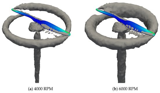
Figure 10.
Q-Criterion Contours (15,000 ).
The wake for UVLM is visualized as the free vortex sheet that is shed from the trailing edge of the rotor. The UVLM is showing the evolution of an instantaneous non-steady state wake while CFD simulations show results for steady state. Unlike CFD wakes, UVLM does not show significant differences between wakes at different angular velocities. Both CFD and UVLM predict similar results to those theoretical wake descriptions found in the literature ([17,23]). A strong vortex structure at the tip of the blade on both CFD and UVLM simulations is evident (see Figure 10 and Figure 11). However, a descending helical path of the tip and inner vortex can be appreciated on CFD simulations because of the application of Q criterion to visualize this phenomena; in contrast, the UVLM method presents a helical path that is clear only at the near wake.
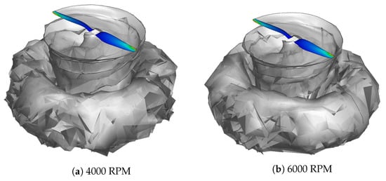
Figure 11.
UVLM wake prediction.
4.2. Pressure Coefficient Distribution on the Rotor
For CFD, is calculated with Equation (15), where is the tip velocity of the blade and is the value set at the pressure inlet boundary condition. Figure 12 shows the distribution of on the surface of the rotor. The variation of for 4000 and 6000 RPM is minor. The maximum at the tip of the rotor is and for 4000 RPM and 6000 RPM, respectively.
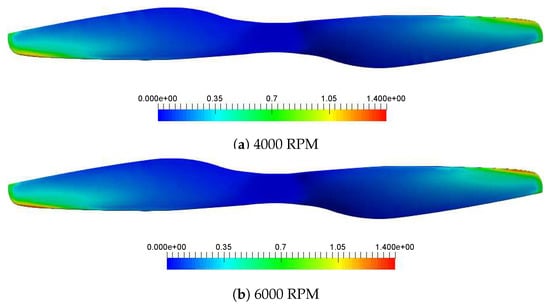
Figure 12.
Contours from CFD simulations.
distribution for UVLM is shown in Figure 13. The pressure distribution is similar to those found in CFD simulations. The main difference between CFD countours and UVLM lays on a purely visualization effect due to discretizations, i.e., a fine surface mesh of the rotor for CFD and the coarse discretization of the surface for the UVLM. In this case, UVLM predicts a maximum of for 4000 RPM and for 6000 RPM; both values are higher than those predicted by CFD.
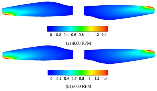
Figure 13.
Contours from UVLM simulations.
4.3. Thrust
First, the estimated angular velocity of the motor (calculated from the PWM signal) is compared to the angular velocity measured by the photo-transistor. Figure 14 exposes that, at low angular velocities, the difference between the estimated and measured is small, but at higher values the difference is considerable and keeps increasing as velocity rises. The model used to estimate the angular velocity of the motor from the PWM signal is applicable only when unloaded. Therefore, experimental results from hereafter are presented using the measured angular velocity. The maximum set rotational velocity of the motor was 6000 RPM, meaning a measured velocity of 5360 RPM. Higher velocities were not tested due to limitations of the power supply source.
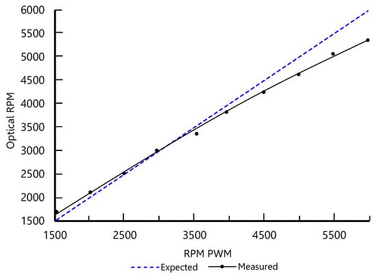
Figure 14.
Calculated RPM vs. Measured RPM.
Thrust generated by the rotor at different rotational velocities through experimental and computational tests is shown in Figure 15. The maximum experimental thrust generated by the rotor was 10 N at 5360 RPM. The highest thrust uncertainty was N for a developed thrust of N at 5069 RPM. It is clear that both CFD and UVLM slightly overpredict the thrust generated by the rotor, though the error seems to diminish at higher angular velocities. Differences between computational and experimental results could be due to the interaction of the structure that supports the motor-rotor system and the wake developed by the rotor. At 6000 RPM, the difference between CFD and UVLM thrust predictions is less than .
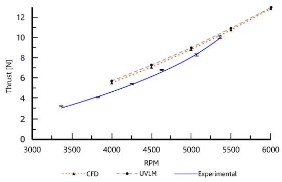
Figure 15.
Experimental and computational thrust.
4.4. Torque
The maximum experimental torque generated by the rotor was N·m at 5360 RPM, as shown in Figure 16. Experimental data shows a maximum uncertainty of N·m for a developed torque of N·m. It is evident that the experimental measurements of torque is between the numerical results from CFD and UVLM simulations, where UVLM underestimates and CFD overestimates torque generated by the rotor. CFD differences with respect to experimental results could be due simplifications of the computational model, where the support structure is not modeled, and also the low order accuracy of the convective terms discretization for the turbulence model equations. Figure 16 spotlights small differences between UVLM and experimental data at low angular velocities; meanwhile, at velocities close to 6000 RPM, this difference increases. Thus, an difference between UVLM and CFD at 6000 RPM is evident.
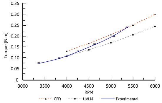
Figure 16.
Experimental and computational torque.
The tip vortices’ core growth rate developed at low angular velocities is smaller than those found at high velocities. This is clearly a mathematical behavior that affects the torque predictions of the UVLM model with viscous correction at high rotational velocities. Then, a variable value of , depending on , is suggested when calculating the turbulent viscosity coefficient (see Section 2.2.1).
Experimental torque measurements at high angular velocities are closer to those calculated through CFD simulations, due to less significant dissipative effects of the turbulent viscosity on the turbulence model at high rotational velocities.
In general, numerical results for both torque and thrust agree well with other results presented in Refs. [24,25,26,27].
4.5. Figure of Merit
Figure of merit () relates the induced power to the actual power (). Induced power, which is the ideal power that the rotor could induce as kinetic energy to the air, is estimated by means of thrust values, based on momentum theory as described in Ref. [17] (Equation (22)), while the actual power is calculated as , where Q is the torque and is the angular velocity:
In Equation (22), T is the thrust, is the density and A is the area of the disk generated by the rotor.
The figure of merit is a parameter used to estimate the efficiency of a rotor operating at hover, and it also works as a useful comparison tool when different rotors operate at same disk loading conditions (). Figure 17 compares the predicted by CFD and UVLM simulations and figure of merit calculated from experimental data. A maximum value of was obtained from experimental data for N/m. The maximum uncertainty is presented at low values of and decreases as disk loading condition increases. CFD simulations slightly overestimate the figure of merit, but the difference with experimental results is lower if the rotor operates at higher . UVLM overestimates figure of merit values over a complete range of disk loading, possibly because of the overprediction of thrust values along the entire angular velocity range. The differences of the figure of merit estimated by UVLM range around .
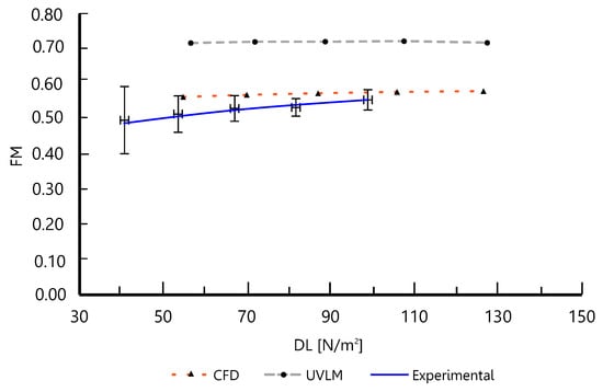
Figure 17.
Figure of merit.
4.6. Flight Time Estimation
Given the operational nature of these kind of vehicles, flight autonomy and energy efficiency are then an important parameter when planning missions. An energy efficiency study allows for estimating the flight time in a simple mission of hover flight only. A simplified model of a complete quadcopter (four rotors) where aerodynamic interaction between rotors and fuselage is not taken into account, the battery (5000 mAh) discharge rate and voltage (15 V) remain constant and the motor efficiency ( ) does not vary with angular velocity was implemented. The total efficiency of the propulsion system was calculated by , whichever the case. Results of flight time as function of load are shown in Figure 18. An overestimation in both UVLM and CFD results when compared to experimental data is observed, as expected. It is evident that the flight time decreases by the square of the load because of the power requirements of the system.
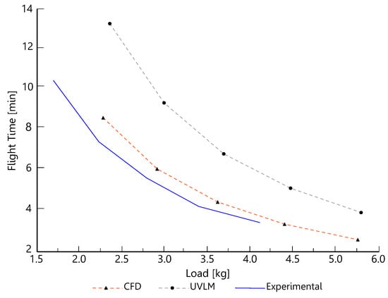
Figure 18.
Flight time.
5. Conclusions
Successful simulations of the flow developed by a small rotor at hover were achieved using two different computational methods, CFD and UVLM. From simulation results, it was possible to study the flow field and the rotor aerodynamic performance. UVLM shows the wake directly as a result of the shed of vortex sheets from the trailing edge of the rotor surface, though there is not a strong difference in the visualization of the wake for different rotational velocities. Wake visualization for CFD simulations was achieved using Q-criterion contours showing stronger tip vortices for higher angular velocities. Predictions of the pressure coefficient distribution along the blade are similar for both methods within the same range. Although UVLM shows a larger zone with a high value of , this may be a consequence of a coarse discretization effect.
Experimental validation determined that both computational methods slightly overestimate the thrust; however, the difference in predictions between them are less than 1%. Experimental torque measurements are closer to CFD predictions at high angular velocities because of the dissipative effects of the turbulence model, while UVLM torque predictions are closer at lower angular velocities due to a stronger dissipative effect of the viscous correction implementation. Figure of merit calculated from CFD simulations is close to experimental measurements, but the UVLM overpredicts the figure of merit by 25%. Differences between computational and experimental results could be due to the low order accuracy of the convective terms of the discretization for the turbulence model equations; in addition, the support structure of the motor–rotor system could impact the performance of the rotor.
A very simple model for the estimation of hover flight time was proposed and discussed. Results from this model show that predictions of the thrust and torque with CFD are closer to the actual flight time, so that numerical results from the implemented UVLM need to be improved.
Author Contributions
Conceptualization, A.M.P.G., O.D.L. and J.A.E.; Formal Analysis, A.M.P.G.; Investigation, A.M.P.G.; Methodology, A.M.P.G., J.S.V.S., O.D.L., L.J.S.C. and J.A.E.; Supervision, O.D.L. and J.A.E.; Validation, J.S.V.S. and L.J.S.C.; Writing—Original Draft, A.M.P.G. and L.J.S.C.; Writing—Review and Editing, O.D.L.
Funding
Departamento Administrativo de Ciencia, Tecnología e Innovación (COLCIENCIAS), Conv. 647, 2014.
Acknowledgments
The authors would like to thank the Departamento Administrativo de Ciencia, Tecnología e Innovación (COLCIENCIAS) and its program to sponsor PhD students in Colombia, also to the high performance computing center at Universidad de los Andes for providing the computational resources, and to ADVECTOR for being part of this research sharing their technical data.
Conflicts of Interest
The authors declare no conflict of interest.
References
- Gordillo, A.M.P. Comparison between Semiempirical and Computational Techniques in the Prediction of Aerodynamic Performance of the Rotor of a Quadcopter. In Aerial Robots; Mejia, O.D.L., Gomez, J.A.E., Eds.; IntechOpen: Rijeka, Croatia, 2017; Chapter 4. [Google Scholar]
- Doerffer, P.; Szulc, O. Numerical Simulation of Model Helicopter Rotor in Hover. Task Q. 2008, 12, 227–236. [Google Scholar]
- Krishna, P.; Kumar, U.; Gaurav, K.; Dhrubajyoti, D.; Dipankar, D.; Anand, S. CFD Analysis of an Isolated Main Helicopter Rotor for a Hovering Flight at Varying RPM. In Proceedings of the ASME 2012 International Mechanical Engineering Congress and Exposition, Houston, TX, USA, 9–15 November 2012. [Google Scholar]
- Sebastian, G.; Lindsay, G.; Bryan, K.; Svetlana, P. Computational Analysis of a Tip Vortex Structure Shed from a Bio-inspired Blade. In Proceedings of the 32nd AIAA Applied Aerodynamics Conference, Atlanta, GA, USA, 16–20 June 2014. [Google Scholar]
- Jiang, Y.; Zhang, B. Numerical Investigation of Effect of Parameters on Hovering Efficiency of an Annular Lift Fan Aircraft. Aerospace 2016, 3, 35. [Google Scholar] [CrossRef]
- Karthikeyan, D.; Baeder, J.D. High Resolution Wake Capturing Methodology for Hovering Rotors. J. Am. Helicopter Soc. 2007, 52, 110–122. [Google Scholar]
- Caradonna, F.X.; Tung, C.F. Experimental and Analytical Studies of a Model Helicopter Rotor in Hover; NASA: Washington, DC, USA, 1981.
- Mark, P.; Thomas, P. Turbulence Modeling Treatment for Rotocraft Wakes. In Proceedings of the AHS Specialists’ Conference on Aeromechanics 2008, San Francisco, CA, USA, 23–25 January 2008. [Google Scholar]
- Yoon, S.; Lee, H.C.; Pulliam, T.H. Computational Analysis of Multi-Rotor Flows. In Proceedings of the 54th AIAA Aerospace Sciences Meeting, San Diego, CA, USA, 4–8 January 2016. [Google Scholar]
- Yang, F.; Xue, X.; Cai, C.; Sun, Z.; Zhou, Q. Numerical Simulation and Analysis on Spray Drift Movement of Multirotor Plant Protection Unmanned Aerial Vehicle. Energies 2018, 11, 2399. [Google Scholar] [CrossRef]
- Szymendera, C. Computational Free Wake Analysis of a Helicopter Rotor; Pennsylvania State University: Philadelphia, PA, USA, 2002. [Google Scholar]
- Shreyas, A. Analysis of Rotor Wake Aerodynamics During Maneuvering Flight Using a Free-Vortex Wake Methodology; University of Maryland: College Park, MD, USA, 2006. [Google Scholar]
- Colmenares, J.; López, O.; Preidikman, S. Computational Study of a Transverse Rotor Aircraft in Hover Using the Unsteady Vortex Lattice Method. Math. Prob. Eng. 2015, 2015, 478457. [Google Scholar] [CrossRef]
- Menter, F.R. Two-equation Eddy-Viscosity Turbulence Models for Engineering Applications. AIAA J. 1994, 32, 1598–1605. [Google Scholar] [CrossRef]
- Menter, F.R.; Langtry, R.B.; Likki, S.R.; Suzen, Y.B.; Huang, P.G.; Völker, S. A Correlation-Based Transition Model Using Local Variables—Part I: Model Formulation. J. Turbomach. 2006, 128, 413–422. [Google Scholar] [CrossRef]
- Varistas, G.H.; Kozel, V.; Mih, W.C. A Simpler Model for Concentrated Vortices. Exp. Fluids 1991, 11, 73–76. [Google Scholar] [CrossRef]
- Leishman, G. Principles of Helicopter Aerodynamics; Cambridge University Press: Cambridge, UK, 2008. [Google Scholar]
- Mahendra, B.; Leishman, G. Generalized Viscous Vortex Model for Application to Free-Vortex Wake and Aeroacoustic Calculations. In Proceedings of the 58th Annual Forum and Technology Display of the American Helicopter Society International, Montreal, QC, Canada, 11–13 June 2002. [Google Scholar]
- Timer, R. Rctimer 5010-530 KV Multicopter Brushless Motor. Available online: http://rctimer.com/product-575.html (accessed on 25 February 2018).
- RCbemchmark. Thrust Stand and Dynamometer. Available online: https://www.rcbenchmark.com/dynamometer-series-1580/ (accessed on 30 September 2018).
- Picard, A.; Davis, R.S.; Gläser, M.; Fujii, K. Revised Formula for the Density of Moist Air (CIPM-2007). Metrologia 2008, 45, 149. [Google Scholar] [CrossRef]
- Holmen, V. Methods for Vortex Identification. Master’s Thesis, Lund University, Lund, Sweden, 2012. [Google Scholar]
- Seddon, J. Basic Helicopter Aerodynamics; Wiley: Hoboken, NJ, USA, 1990. [Google Scholar]
- Kotwani, K.; Sane, S.; Arya, H.; Sudhakar, K. Experimental Characterization of Propulsion System for Mini Aerial Vehicle. In Proceedings of the 31st National Conference on Fluid Mechanics and Fluid Power, Kolkata, India, 11–13 December 2003. [Google Scholar]
- Smedresman, A.; Arbor, A.; Yeo, D.; Shyy, W. Design, Fabrication, Analysis, and Dynamic Testing of a Micro Air Vehicle Propeller. In Proceedings of the 29th AIAA Applied Aerodynamics Conference, Honolulu, HI, USA, 27–30 June 2011. [Google Scholar]
- Brezina, A.; Thomas, S. Measurement of Static and Dynamic Performance Characteristics of Electric Propulsion Systems. In Proceedings of the 51st AIAA Aerospace Sciences Meeting including the New Horizons Forum and Aerospace Exposition, Grapevine, TX, USA, 7–10 January 2013. [Google Scholar]
- Intaratep, N.; Alexander, W.N.; Devenport, W.J.; Grace, S.M.; Dropkin, A. Experimental Study of Quadcopter Acoustics and Performance at Static Thrust Conditions. In Proceedings of the 22nd AIAA/CEAS Aeroacoustics Conference, Lyon, France, 30 May–1 June 2016. [Google Scholar]
© 2019 by the authors. Licensee MDPI, Basel, Switzerland. This article is an open access article distributed under the terms and conditions of the Creative Commons Attribution (CC BY) license (http://creativecommons.org/licenses/by/4.0/).