Dynamically Coupled Operation of Two-Tank Indirect TES and Steam Generation System

Abstract

A thermal energy storage system is a critical component in concentrating solar power plants (CSPP), owing to which concentrating solar power (CSP) has superiorities over photovoltaic and wind power. Currently, the sole thermal energy storage (TES) system which is commercially applied to parabolic trough solar power (PTSP) plants worldwide is the two-tank indirect TES. In this study, the dynamic models of a solar field (SF), a two-tank indirect TES system, and a steam generation system (SGS) in a PTSP plant were developed and validated. Control and operation strategies on a clear day and a cloudy day were provided, and the dynamic simulations of the coupled operation using actual meteorological data were conducted. The influence of the two-tank indirect TES system on the dynamic characteristics of SGS on a system level was analyzed. Other key parameter variations were also presented. The results show that during the transition from the charge to the discharge process, the steam parameters slowly decrease. The variation of the molten salt height is further affected by the molten salt mass flow rate at the inlet and outlet of the molten salt tank. We adopted the PI control to adjust the thermal oil mass flow rate, thermal oil temperature, and water height. The developed dynamic models are useful in guiding system operation and control.

1. Introduction

With the increasing prosperity in fast-growing and emerging economies, the world GDP is expected to be more than double by 2040, which will drive an increase in global energy demand [1]. According to the BP Energy Outlook 2018 [1], renewable energy will account for 40% of the growth in primary energy and be the fastest growing energy source. 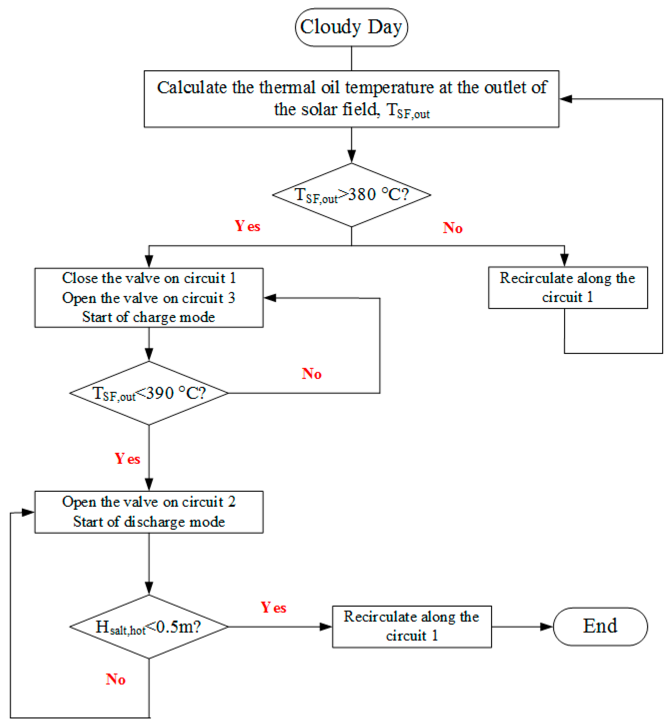As a renewable energy utilization technology, CSP technology is increasingly emphasized by more countries, especially by those who are rich in solar energy resources [2]. This type of technology has superiorities over others due to its ability to integrate a TES system. This system mitigates weak fluctuations in ephemeral weather conditions. For instance, during cloudy periods, it shifts from the peak time of solar radiation to that of electricity demand. Also, it extends the generating period when there is no solar resources, i.e., nighttime [3].

Until now, there are four different kinds of concentrating solar power plants (CSPPs): solar energy towers, parabolic trough solar power (PTSP), solar dish Stirling engines, and linear Fresnel reflector solar power [4]. Among them, PTSP world-wide is the oldest and the most mature CSP technology [5]. According to the National Energy Technology Laboratory (NREL, Golden, CO, USA) [6], all commercial operational PTSP all over the world adopts a two-tank indirect TES with molten salt. Because of the irregularity of the solar radiation, the SGS output varies throughout the day, which leads to fluctuations in its electricity production. Hence, for a PTSP plant, it is essential to investigate ways to mitigate fluctuations and extend the generation period with a two-tank indirect TES system.

Some literature focused on the system-level coupled operation of a TES system and SGS in a technical and/or economic aspect. Kolb [7] compared the annual performance of 50-MWe Andasol-like PTSP plants integrated with a thermocline-type or two-tank molten-salt TES system using TRNSYS software. The results revealed that if the temperatures approach the required design points, the two-tank TES performs significantly better than the thermocline TES. Powell and Edgar [8] considered the effect of a two-tank direct TES system on the power output of a PTSP plant. A solar collector model, a two-tank direct TES model, and a boiler model were developed as well as a control strategy was provided. The simulation results showed that the TES system allowed the plant to produce power at a constant rate on a cloudy day with intermittent solar radiation and it also increased the solar share of the plant and reduced the need for supplementary fuel. Flueckiger et al. [9] developed a new thermocline-type tank model as well as integrating it into a systematic model of a 100-MWe energy tower plant. A plant simulation in a meteorological year was conducted with the results showing that the thermocline tank raised the plant capacity factor yearly and provided excellent storage performance. Biencinto et al. [10] performed an annual performance analysis of a solar energy plant with thermocline-type storage tank. Different operation strategies were developed, and their advantages and disadvantages were identified by system-level simulations. The simulation results provided references for a further economic assessment of thermocline storage systems. Suresh et al. [11] presented a detailed methodology in sizing a solar field for a PTSP with a two-tank molten- salt storage system. The yearly electricity generated based on the specified hours of TES was determined, and the solar field size was adjusted for yearly maximum solar-to-electric conversion effectiveness. Luca et al. [12] analyzed a PTSP plant with various configurations according to its multiple solar storage capacities and obtained the economically optimal configurations. Rodríguez et al. [13] assessed a TES solution for a 1-MWe CSP-ORC solar power plant in technical and economic points of view. They also presented detailed ephemeral models of a two-tank TES system and a thermocline-type storage system. The effects of each TES system on the technical and economic performance of the plant were investigated and compared by annual simulations. Chacartegui et al. [14] analyzed a PTSP plant incorporated with a cycle power block (Organic Rankine) along with thermal storage. They investigated these two different thermal storage integrations and showed full system performance under design and off-design conditions. Andika et al. [15] conducted a techno-economic assessment of the technological progress in the TES of a CSP. Cases were generated by combining two kinds of thermal storage tanks, two kinds of thermal storage media, as well as two kinds of power cycles. The influence of each technological improvement was also analyzed. Rohani et al. [16] modeled a commercial PTSP plant with a two-tank indirect TES system and corresponding control strategies. Based on the real operation boundaries, systematic simulations were conducted, and the results were compared with the operating data. Cioccolanti et al. [17] investigated a concentrated solar cycle plant (Organic Rankine) coupled with a phase transition material storage tank. Particularly, they also evaluated the effect of several operation modes on the model plant performance. Fasquelle et al. [18] simulated a 50-MWe energy plant with a thermocline tank storage and provided the best control strategy. In addition, the annual performance of the thermocline technology was compared with that of the two-tank technology.

Some literature focused on the control scheme for PTSP plants. Fontalvo et al. [19] developed a non-linear dynamic model of a hybrid solar-fossil energy power plant and presented a comprehensive study of three control schemes to maintain the steam temperature approximately at its set point. Guo et al. [20] developed a nonlinear dynamic model of SF for a direct steam generation PTSP plant. Based on the proposed model, a novel predictive control scheme of multi-model switching is developed for the simulated control of plant behavior in various operational conditions. Rodat et al. [21] put forward a CSP plant-based dynamic model combined with Fresnel SF, a double-media thermocline tank and an Organic Rankine cycle. With it, the control problem of the solar field outlet temperature was analyzed.

In the aforementioned literature, the system-level analyses of coupled operation of the TES system and SGS were conducted; however, two aspects should be further considered. Firstly, the boundary condition model-SF model or SGS model is either a steady model or an empirical model, not a dynamic model. A dynamic model is more suitable in the analysis of a CSP plant operation due to its more obvious dynamic characteristics than those of conventional power plants. Secondly, thermocline storage or phase change material storage is more attractive to researchers, but two-tank indirect TES with molten salt is the only technology commercially used in a PTSP plant. Research and evaluation of the system control and operation strategies are of practical interest. In this study, the dynamic models of the SF, SGS, together with two-tank molten-salt indirect TES system were developed and integrated for the first time. The modeling methods are provided in detail, and the models are validated by experiment or reference data. Control and operation strategies on a clear day and a cloudy day are provided and validated by system-level dynamic simulations, which provides a valuable reference for a plant operator. These are the contributions of this study.

2. System Description

In this study, the Yanqing 1-MWe CSP plant was used as the case to analyze the influence of a two-tank indirect TES system on the dynamic characteristics of SGS. This plant is located at Badaling Town in the Yanqing District in Beijing. Its geographic coordinates are latitude 40°22’48” N, longitude 115°56’24” E. The plant schematic and its images are shown in Figure 1 and Figure 2, respectively. As shown in Figure 1, the plant comprises of four parts: an SF, a two-tank indirect TES system, an SGS, and a power block. SF includes three 600-m long loops. Loop 1 and Loop 2 have East-West layouts, and Loop 3 has a North-South layout. A superheater, an evaporator and a preheater are included in SGS. When SF is operating, the heat transfer fluid (HTF) first recirculates along Circuit 1. HTF flows through the receiver, which is anchored at the focusing line of the trough, and it absorbs the solar radiation energy gathered by the concentrator, increasing its temperature. After the HTF temperature at SF outlet reaches its minimum value, it starts to flow along Circuit 2. The water in the SGS absorbs the heat exuded by the HTF and becomes superheated steam. Then the steam drives the turbine to generate electricity. When there is surplus energy in SF, the HTF will deliver the extra heat into the storage medium in the TES system by flowing along Circuit 3. When the energy in SF is insufficient, the HTF will flow reversely along the Circuit 3 and absorb the heat exuded by the storage medium. The HTF in SF is thermal oil, the storage medium is molten salt. The power block consists of a turbine generator, a condenser and a deaerator, which are the same as those in a conventional power plant. The rated operation parameters are also indicated in Figure 1.

3. Modeling Method

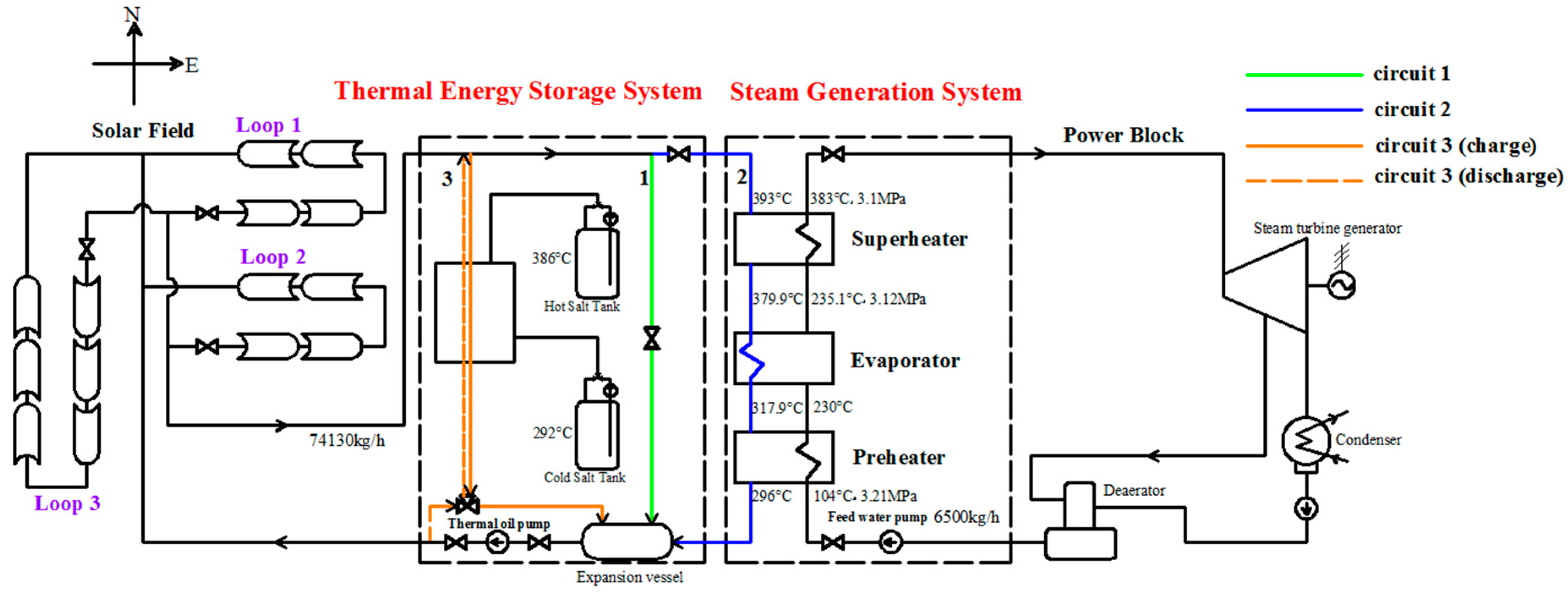
This study focused on the influence of a two-tank indirect TES system on the dynamic characteristics of the SGS; hence, the steam turbine generator model was a simple model, and only the dynamic models of the SF, two-tank indirect TES system, and SGS were developed in detail. The modeling methods will be described in this chapter.

3.1. SF

The SF in Yanqing PTSP plant consists of three loops.

Table 1. The main SF design parameters.

Component	Parameters	Value
Collector	Width (m)	5.776
	Length (m)	100/150
	Focal length (m)	1.71
	Clean mirror reflectivity (-)	0.96
	Ideal intercept factor (-)	0.8268
Receiver	Inner diameter of the absorber (m)	0.064
	Outer diameter of the absorber (m)	0.07
	Absorptivity of the absorber (-)	0.95
	Emissivity of the absorber (-)	0.08 (100 °C), 0.14 (400 °C)
	Inner diameter of the envelope (m)	0.114
	Outer diameter of the envelope (m)	0.12
	Transmissivity of the envelope (-)	0.95
	Absorptivity of the envelope (-)	0.02
	Emissivity of the envelope (-)	0.9

gives the main SF design parameters. The SF models include a solar collector assembly (SCA) model and a receiver model, which were developed separately.

3.1.1. The SCA Model

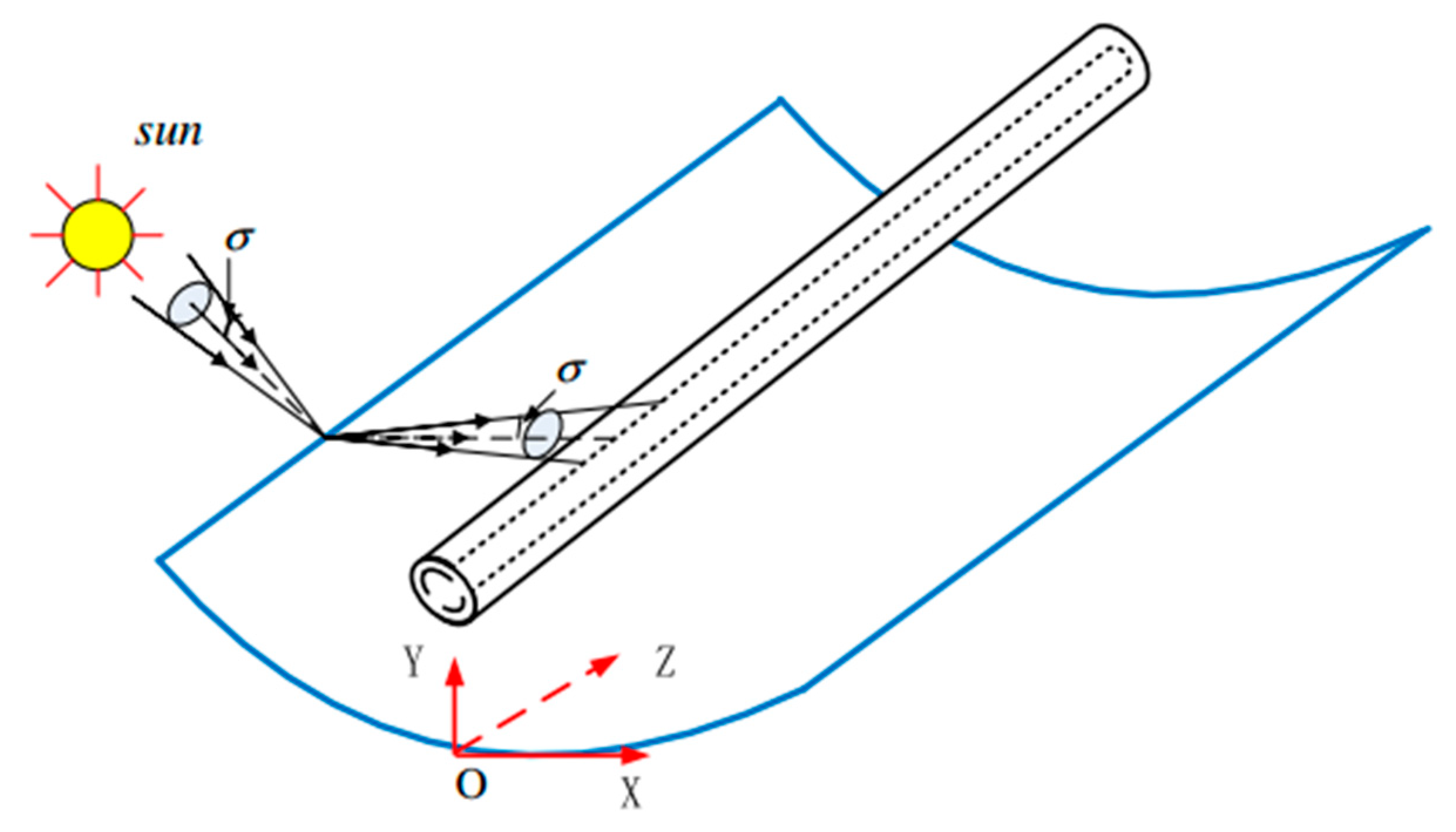
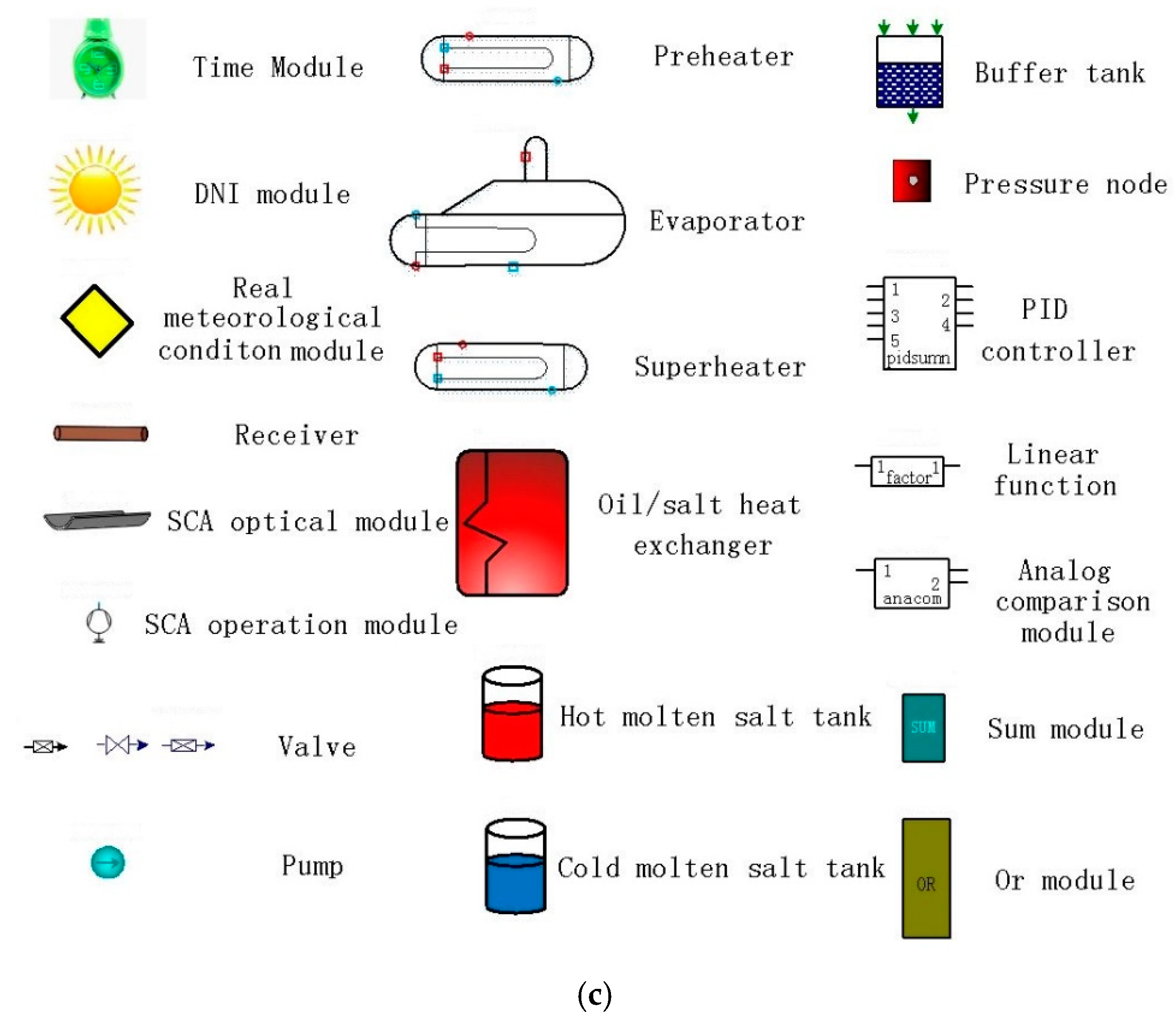
The SCA model includes a direct normal irradiation (DNI) model, an SCA operational model, and an SCA optical model. Among them, the SCA optical model is most important, which is developed on the basis of the Monte Carlo Ray Tracing (MCRT) method and the coordinate transformation method. The SCA optical model can simulate the flux distribution on the receiver accurately. The schematic of the SCA is shown in Figure 3, where σ represents the angular radius of the solar beam. MCRT method is to calculate and simulate the corresponding reflected rays by determining the position of the incident rays, and then count the number of rays and calculate the energy flux density in the region. The coordinate transformation method can give the relation between the incident rays and reflected rays. The detailed modeling method is not provided here due to the length of the study; however, it can be referred to in reference [22].

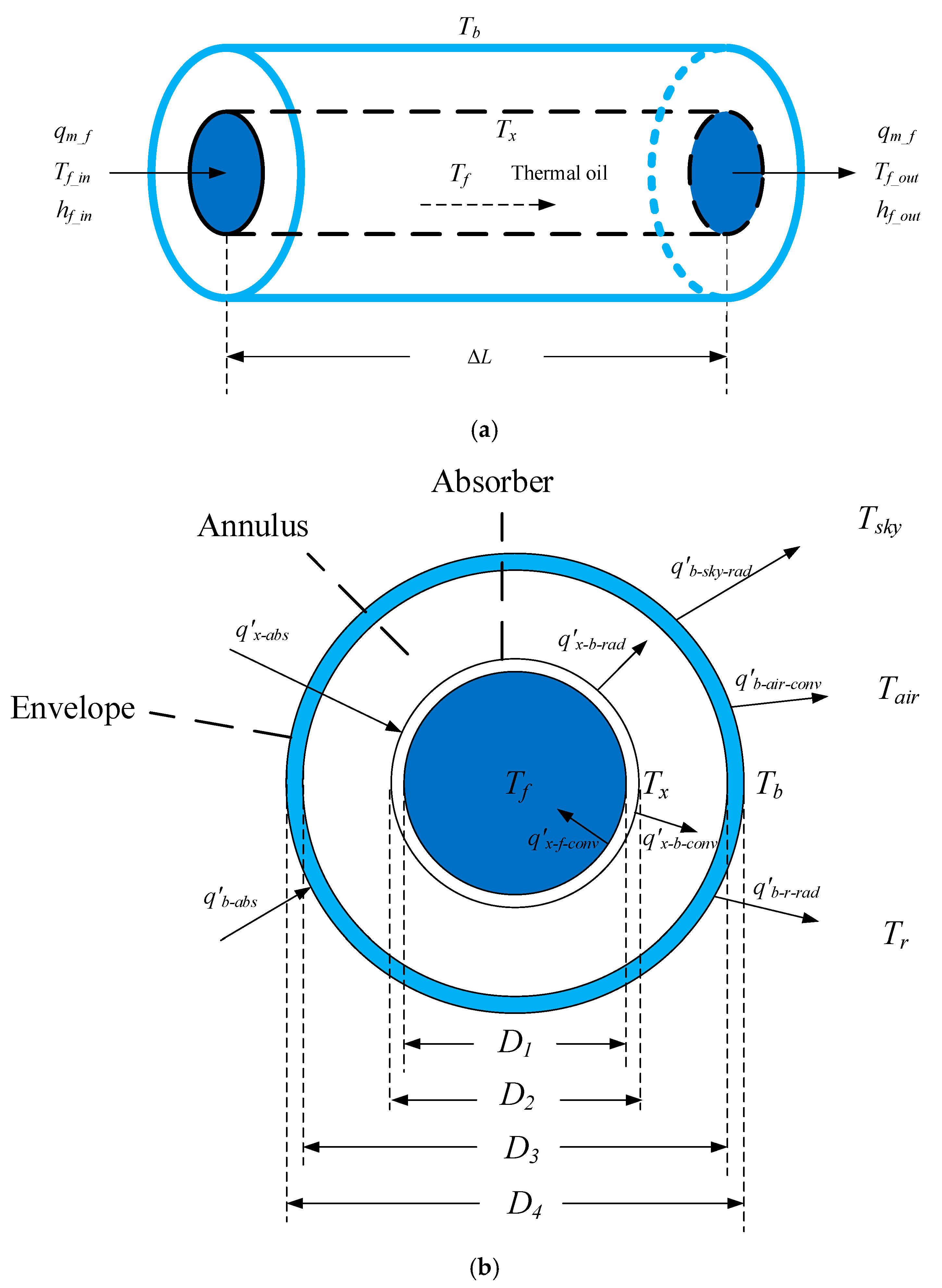
3.1.2. The Receiver Model

The receiver consists of an absorber, an envelope, and an annulus between them. To establish the receiver model, the hypotheses are made as follows:

• The temperature gradient in a radial direction is neglected because the geometrical size of the receiver in the radial direction is tiny relative to the axial direction. Therefore, the inner and outer wall temperatures of the absorber are equal. The inner and outer wall temperatures of the envelope are also identical.
• The proportion of the length of the bellow and bracket to the total receiver length is relatively small; therefore, they and the receiver are taken as a whole.

The receiver is evenly divided into N parts each with a length of ΔL. The energy balance equations for the receiver unit with ΔL length are then listed. The schematic of the receiver model is shown in Figure 4.

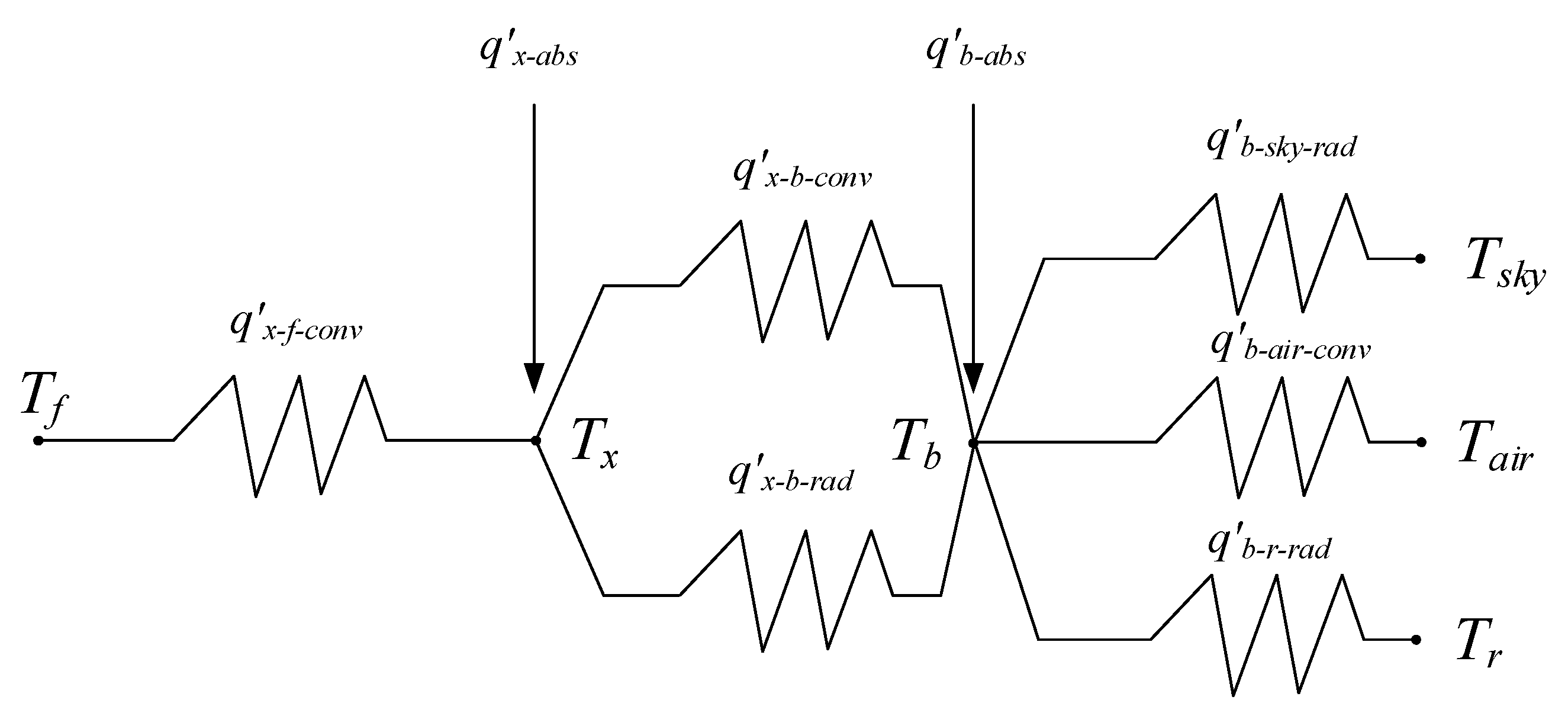
Based on the energy balance, the heat resistance network is obtained as shown in Figure 5. From Figure 5, the radiation from the envelope to the reflector is considered.

The heat transmission between the absorber and thermal oil is considered as convection heat transfer. The convective heat flux per unit axis length is calculated as follows:

$$q_{x-f-conv}^{\prime }={\alpha }_{x-f}{D}_{12}\pi (T_x-T_f)$$

(1)

where D₁₂ is the arithmetic mean of the internal and external diameter of the absorber, T_f is the arithmetic mean of the thermal oil temperature at the outlet and inlet, and the heat transfer coefficient α_x−f is obtained by the Gnielinski correlation [23], which is given in Appendix A.

The heat flux per unit length of axis absorbed by an absorber is computed as follows.

$$q_{x-abs}^{\prime }=\overline{q}\pi D_{12}$$

(2)

Here, $\overline{q}$ is the average energy flow density in the absorber circumference, which comes from the reflector.

The heat transmission between the envelope and absorber mainly includes two parts: heat radiation and heat convection. The radiation from the exterior wall of the absorber to the interior wall of the envelope is as follows.

$$q_{x-b-rad}^{\prime }=\frac{\pi D_{12}{\sigma }_s(T_x{}^4-T_b{}^4)}{\frac{1}{{\epsilon }_x}+\frac{(1-{\epsilon }_b)D_{12}}{{\epsilon }_b{D}_{34}}}$$

(3)

Here, σ_s is the Stefan-Boltzmann constant, which is 5.67 × 10⁻⁸ W/(m²·K⁴), ε_x is the emissivity of the absorber, and ε_b is the emissivity of the envelope. D₃₄ is the arithmetic mean value of the internal and external diameter of the envelope.

When the pressure in the annulus is less than 1 torr (1 torr = 133.322 Pa), free molecular heat transfer describes the convective heat loss between the annulus and absorber. This free molecular heat transfer is calculated as follows [24]:

$$q_{x-b-conv}^{\prime }={\alpha }_{x-b}{D}_{12}\pi (T_x-T_b)$$

(4)

The computation of the free molecular heat transfer coefficient α_x−b is given in Appendix A.

When the pressure in the annulus is above 1 torr, the convective heat transfer is considered for the heat loss between the annulus and absorber. The convective heat transfer is computed as follows [24]:

$$q_{x-b-conv}^{\prime }=\frac{2.425k{(\frac{PrRa}{0.861+Pr})}^{\frac{1}{4}}(T_x-T_b)}{{\left(1+{(\frac{D_{12}}{D_{34}})}^{\frac{3}{5}}\right)}^{\frac{5}{4}}}$$

(5)

In Equation (5), the arithmetic mean of the absorber temperature and annulus temperature is taken as the qualitative temperature.

The heat flux absorbed by the envelope is computed as follows:

$$q_{b-abs}^{\prime }=\frac{\overline{q}\pi D_{12}}{{\alpha }_x^{\prime }{\tau }_b}{\alpha }_b^{\prime }$$

(6)

where α_x’ is the absorptivity of the absorber, α_b’ is the absorptivity of the envelope, and τ_b is the transmissivity of the envelope.

The radiant heat flow from the envelope to the sky is calculated by

$$q_{b-sky-rad}^{\prime }=x_{sky}\pi D_{34}{\sigma }_s{\epsilon }_b\left(T_b^4-T_{sky}^4\right)$$

(7)

where x_sky is the view factor of the radiation from the envelope to the sky.

The radiant heat flow from the glassy cover tube to the reflector is calculated by

$$q_{b-r-rad}^{\prime }=x_r\pi D_{34}{\sigma }_s{\epsilon }_b\left(T_b^4-T_r^4\right)$$

(8)

The convective heat transfer between the envelope and the environmental air is calculated by

$$q_{b-air-conv}^{\prime }={\alpha }_{b-air}\pi D_{34}\left(T_b-T_{air}\right)$$

(9)

Here, the convective heat transfer coefficient α_b-air depends on the ambient wind speed, which is calculated in Appendix A.

According to the heat resistance network in Figure 5, the energy conservation equations used for the thermal oil in the absorber is expressed as

$$c_{p\_f}{\rho }_f{V}_f\frac{d{T}_f}{dt}=q_{x-f-conv}^{\prime }\cdot \Delta L+q_{m\_f}(h_{f\_in}-h_{f\_out})$$

(10)

where V_f represents the volume of the thermal oil in the absorber, which is calculated by

$$V_f=\frac{\pi D_1^2\cdot \Delta L}{4}$$

(11)

The energy conservation equations used for the absorber is expressed as

$$c_x{\rho }_x{V}_x\frac{d{T}_x}{dt}=\left(q_{x-abs}^{\prime }-q_{x-f-conv}^{\prime }-q_{x-b-conv}^{\prime }-q_{x-b-rad}^{\prime }\right)\cdot \Delta L$$

(12)

where V_x represents the volume of the absorber, which is calculated by

$$V_x=\frac{\pi (D_2^2-D_1^2)\cdot \Delta L}{4}$$

(13)

The energy conservation equations used for the envelope is expressed as

$$c_b{\rho }_b{V}_b\frac{d{T}_b}{dt}=(q_{b-abs}^{\prime }+q_{x-b-conv}^{\prime }+q_{x-b-rad}^{\prime }-q_{b-sky-rad}^{\prime }-q_{b-r-rad}^{\prime }-q_{b-air-conv}^{\prime })\cdot \Delta L$$

(14)

where V_b represents the volume of the envelope, which is calculated by

$$V_b=\frac{\pi (D_4^2-D_3^2)\cdot \Delta L}{4}$$

(15)

From Equations (10)–(15), the developed receiver model in this study can calculate not only the thermal oil temperature at the receiver outlet but also the variations of absorber and envelope temperature with time.

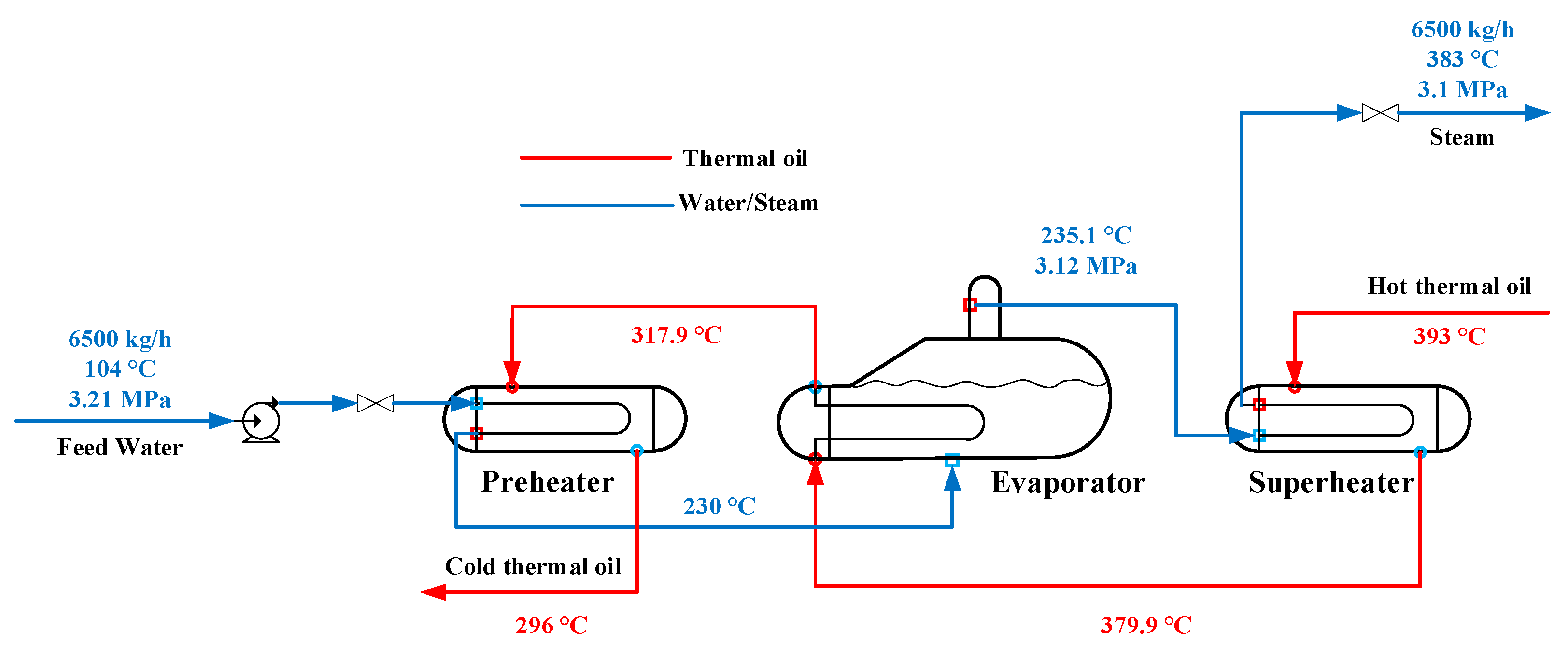
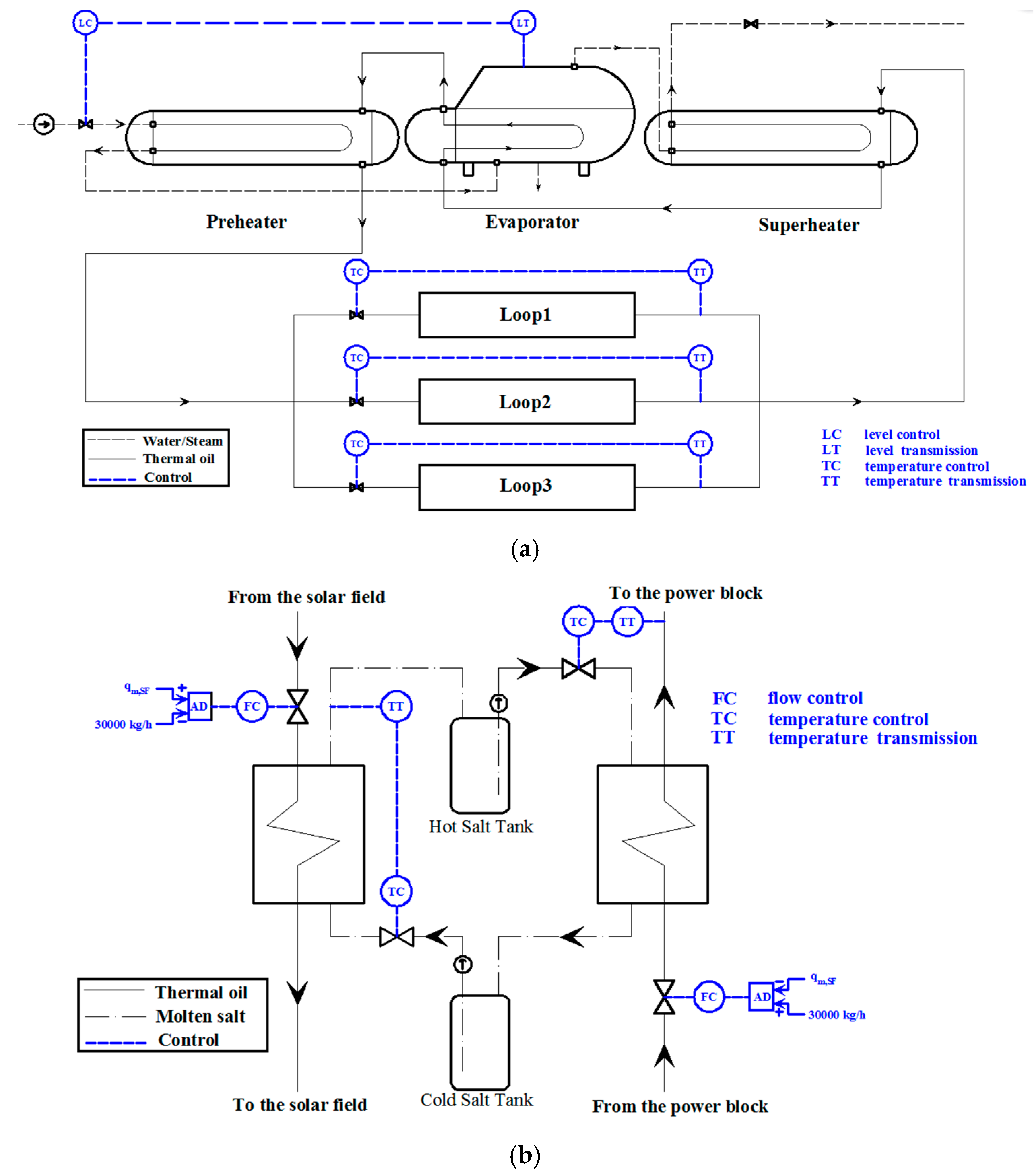
3.2. SGS

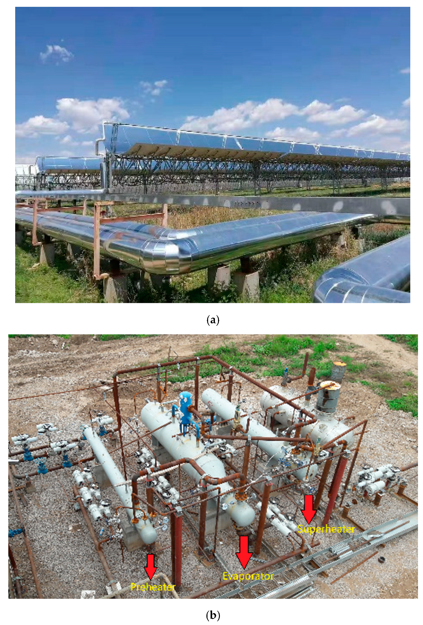
A superheater, an evaporator and a preheater are included in SGS. The design parameters are enumerated in

Table 2. SGS parameters.

Design Parameters	Preheater	Evaporator	Superheater
Tube outer diameter (m)	0.016	0.016	0.016
Tube inner diameter (m)	0.012	0.012	0.012
Number of tube-side passes (-)	4	2	4
Number of shell-side passes (-)	1	1	1
Area of heat transfer (m2)	10	40	47
Tube density (kg/m3)	7850	7850	7850
Tube specific heat capacity (J/(kg·°C))	529	529	529
Tube bundle layout (-)	Triangular	Triangular	Triangular
Single tube length (m)	4	4	4
Tube-side effective volume (m3)	0.063	0.2	0.25
Shell-side effective volume (m3)	0.26	1.86	0.63
Working fluid at the shell side	Thermal oil	Water/Steam	Thermal oil
Working fluid at the tube side	Water	Thermal oil	Steam

.

In this study, the lumped parameter method is adopted to model the preheater, evaporator, and superheater. A representative point in space is selected, and its state parameters represent the system parameters. Figure 6 shows the schematic of the model. The model is developed on the basis of the following hypotheses:

• The working fluid parameters at the middle point in the preheater and superheater are adopted as the lumped parameters.
• The pressure slump at the preheated water side in the preheater and at the oil side in the whole SGS can be ignored.
• The steam and water in the evaporator are in the equivalent thermodynamic condition. They have the same temperature and pressure.
• The steam at the outlet of the evaporator does not carry water.
• Only the thermal storage capacity of the wall is considered, and its thermal conduction is negligible.
• The heat loss between the environmental air and SGS is ignored due to excellent insulation.

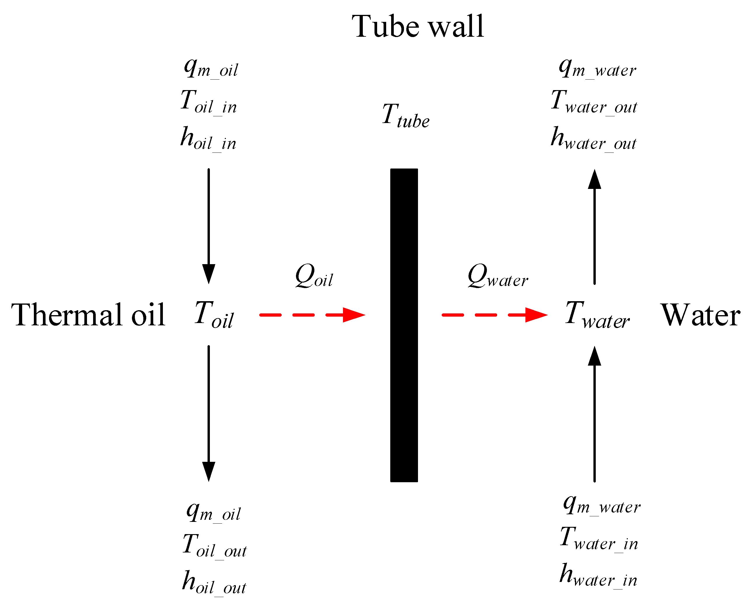
3.2.1. Preheater and Superheater

There is no phase change in the superheater or preheat. The preheater model is divided into three parts: the thermal oil side model, the heat transfer tube wall model, and the preheated water side model. The schematic of the preheater model is shown in Figure 7.

The energy conservation equations at the thermal oil side are given as follows:

$$\frac{d(c_{p\_oil}{m}_{oil}{T}_{oil})}{dt}=q_{m\_oil}(h_{oil\_in}-h_{oil\_out})-Q_{oil}$$

(16)

$$Q_{oil}={\alpha }^{\prime }{A}_o(T_{oil}-T_{tube})$$

(17)

Here, α’ is the convective heat transfer coefficient, obtained by the Zhukauskas correlations [23], which are given in Appendix A.

At the water side, the energy conservation equations are expressed as follows:

$$\frac{d(c_{p\_water}{m}_{water}{T}_{water})}{dt}=q_{m\_water}(h_{water\_in}-h_{water\_out})+Q_{water}$$

(18)

$$Q_{water}=\alpha A_i(T_{tube}-T_{water})$$

(19)

Here, α is the convective heat transfer coefficient, obtained by the Dittus-Boelter correlation [23], which is given in Appendix A.

The heat transfer tube wall model based on energy conservation is given as follows:

$$\frac{d(c_{p\_tube}{m}_{tube}{T}_{tube})}{dt}=Q_{oil}-Q_{water}$$

(20)

Based on the modeling method described above, the superheater model can be obtained by changing the fluid at the tube side into steam. Besides, for a superheater, a steam pressure drop should be considered, which is calculated by Equation (21) [25]:

$$\Delta p_{steam}=(ft\cdot (\Delta p_1+\Delta p_2)+\Delta p_3)\times {10}^{-6}$$

(21)

$$\Delta p_2=4\frac{{\rho }_{steam}{v}_{steam}^2}{2}{n}_t$$

(22)

$$\Delta p_3=1.5\frac{{\rho }_{steam}{v}_{steam}^2}{2}$$

(23)

$$\begin{array}{l}\Delta p_1=\lambda \frac{l}{d_i}\frac{{\rho }_{steam}{v}_{steam}^2}{2}{(\frac{\mu }{{\mu }_w})}^{-0.14}(R{e}_{steam}>2100)\\ \Delta p_1=\lambda \frac{l}{d_i}\frac{{\rho }_{steam}{v}_{steam}^2}{2}{(\frac{\mu }{{\mu }_w})}^{-0.25}(R{e}_{steam}<2100)\end{array}$$

(24)

In Equation (24), λ is the resistance coefficient, which is calculated as follows [26]:

$$\begin{array}{ll}\lambda ={\lambda }_{lam}& (R{e}_{steam}<2000) ,\\ \lambda =\max \left\{{\lambda }_{lam},{\lambda }_{turb}\right\}& (2000\le R{e}_{steam}\le 4000) ,\\ \lambda ={\lambda }_{turb}& (R{e}_{steam}>4000) ,\end{array}$$

(25)

with

$$\begin{array}{l}{\lambda }_{lam}=\frac{64}{R{e}_{steam}} ,\\ {\lambda }_{turb}={(1.82\lg R{e}_{steam}-1.64)}^{-2}.\end{array}$$

(26)

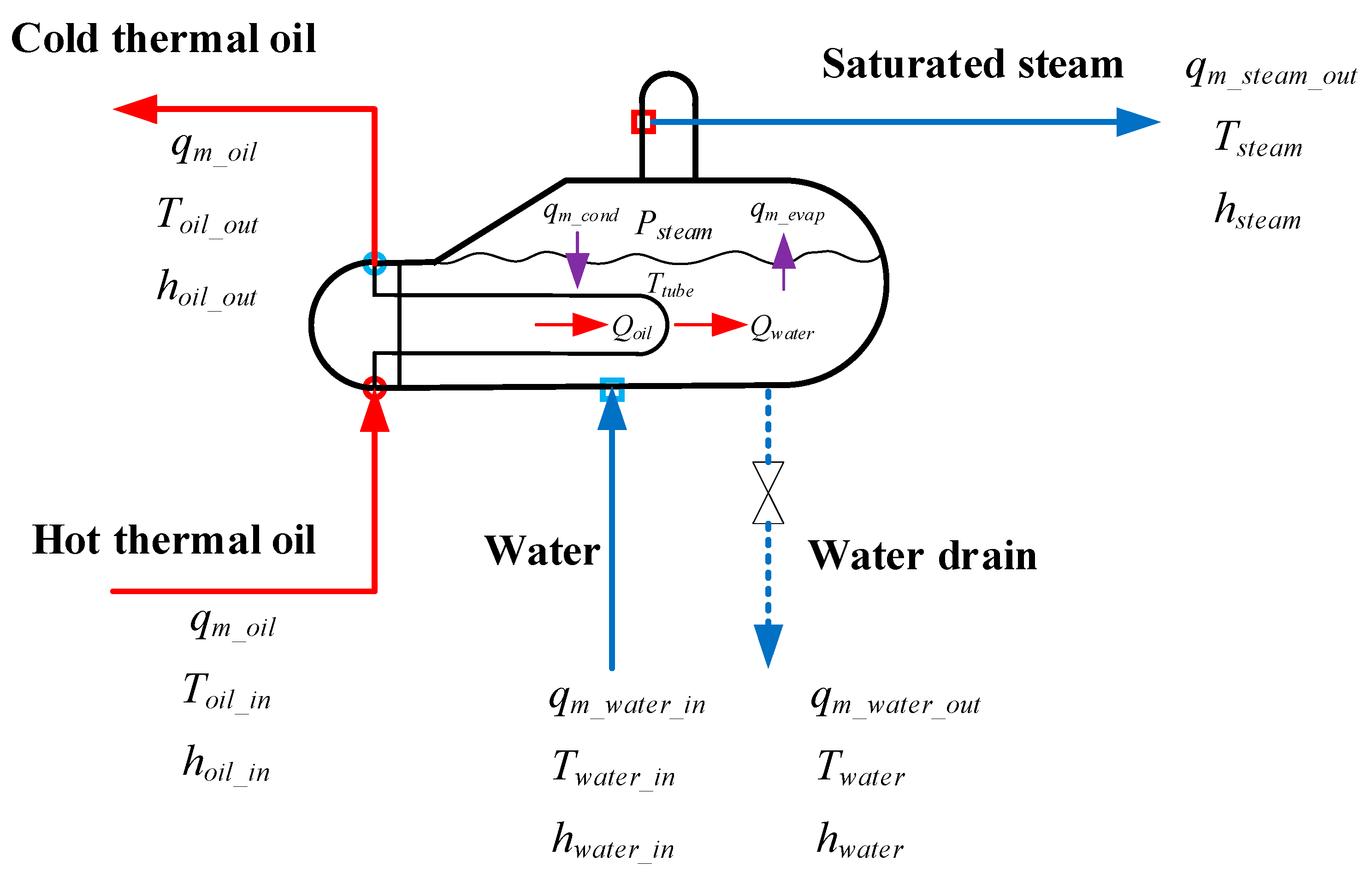
3.2.2. Evaporator

The evaporator belongs to a kettle-type heat exchanger. A phase change occurs at the shell side, so the evaporator modeling is more complicated. Figure 8 shows the schematic of the evaporator model.

The evaporator model consists of four parts: the thermal oil side model, the water/steam side model, the heat transfer tube wall model and the water height model.

The thermal oil side model is obtained based on the energy conservation as follows:

$$\frac{d(c_{p\_oil}{m}_{oil}{T}_{oil})}{dt}=q_{m\_oil}(h_{oil\_in}-h_{oil\_out})-Q_{oil}$$

(27)

$$Q_{oil}=\alpha A_i(T_{oil}-T_{tube})$$

(28)

Here, α is the convective heat transfer coefficient, computed by the Dittus-Boelter correlation, which can be obtained in Appendix A.

The water/steam side model is developed according to the following mass conservation and energy conservation:

For the mass conservation equation,

$$\frac{d({\rho }_{water}{V}_{water}+{\rho }_{steam}{V}_{steam})}{dt}=q_{m\_water\_in}-q_{m\_steam\_out}-q_{m\_water\_out}$$

(29)

$$V_{water}+V_{steam}=V=const$$

(30)

For the energy conservation equation,

$$\frac{d({\rho }_{water}{V}_{water}{h}_{water}+{\rho }_{steam}{V}_{steam}{h}_{steam})}{dt}=q_{m\_water\_in}{h}_{water\_in}-q_{m\_water\_out}{h}_{water}-q_{m\_steam\_out}{h}_{steam}+Q_{water}$$

(31)

Here, the heat exchange for pool boiling Q_water is calculated by the Rohsenow correlation [27], which is given in Appendix A.

Equations (29)–(31) can be transformed into

$$\frac{d{\rho }_{water}}{dt}{V}_{water}+\frac{d{V}_{water}}{dt}{\rho }_{water}+\frac{d{\rho }_{steam}}{dt}{V}_{steam}+\frac{d{V}_{steam}}{dt}{\rho }_{steam}=q_{m\_water\_in}-q_{m\_steam\_out}-q_{m\_water\_out}$$

(32)

$$\frac{d{V}_{water}}{dt}=-\frac{d{V}_{steam}}{dt}$$

(33)

$$\begin{array}{l}(\frac{d{h}_{water}}{dt}{\rho }_{water}+\frac{d{\rho }_{water}}{dt}{h}_{water})V_{water}+(\frac{d{h}_{steam}}{dt}{\rho }_{steam}+\frac{d{\rho }_{steam}}{dt}{h}_{steam})V_{steam}\\ +\frac{d{V}_{water}}{dt}{\rho }_{water}{h}_{water}+\frac{d{V}_{steam}}{dt}{\rho }_{steam}{h}_{steam}\\ =q_{m\_water\_in}{h}_{water\_in}-q_{m\_water\_out}{h}_{water}-q_{m\_steam\_out}{h}_{steam}+Q_{water}\end{array}$$

(34)

Using Equations (32)–(34), the relationship $\frac{d}{dt}=\frac{\partial }{\partial p_{steam}}(\frac{d{p}_{steam}}{dt})$, and eliminating $\frac{d{V}_{water}}{dt}$ and $\frac{d{V}_{steam}}{dt}$, the steam pressure’s variation in the evaporator with time is given by [28]

$$\frac{d{p}_{steam}}{dt}=\frac{Q_{water}+(\frac{r{\rho }_{steam}}{{\rho }_{water}-{\rho }_{steam}}-h_q)q_{m\_water\_in}-\frac{r{\rho }_{steam}}{{\rho }_{water}-{\rho }_{steam}}{q}_{m\_water\_out}-\frac{r{\rho }_{water}}{{\rho }_{water}-{\rho }_{steam}}{q}_{m\_steam\_out}}{\left[{\rho }_{water}\frac{\partial h_{water}}{\partial p_{steam}}+\frac{r{\rho }_{steam}}{{\rho }_{water}-{\rho }_{steam}}(\frac{\partial {\rho }_{water}}{\partial p_{steam}})\right]V_{water}+\left[{\rho }_{steam}\frac{\partial h_{steam}}{\partial p_{steam}}+\frac{r{\rho }_{water}}{{\rho }_{water}-{\rho }_{steam}}(\frac{\partial {\rho }_{steam}}{\partial p_{steam}})\right]V_{steam}}$$

(35)

Here, r is the latent heat of vaporization, $r=h_{steam}-h_{water}$ and h_q is the lower enthalpy of the feed water, $h_q=h_{water}-h_{water\_in}$.

The steam mass flow rates and feed water have a relation with the pressure, which is given by [28]:

$$q_{m\_water\_in}=c\sqrt{p_{water\_in}-p_{steam}}$$

(36)

$$q_{m\_steam\_out}=c^{\prime }{p}_{steam}$$

(37)

Here, c and c’ are the coefficients which are used to calculate the mass flow rate. They are determined by the constant condition.

For the water height model, the steam volume below the water/steam interface should be considered. The equation is given below [28]:

$$H_{water}=(V_{water}+V_{steam\_below})/S=(\frac{m_{water}}{{\rho }_{water}}+V_{steam\_below})/S$$

(38)

where

$$\frac{d{m}_{water}}{dt}=q_{m\_water\_in}+q_{m\_cond}-q_{m\_evap}-q_{m\_water\_out}$$

(39)

$$V_{steam\_below}=a+b{q}_{m\_evap}$$

(40)

Here, $q_{m\_evap}$ is the dynamic water evaporation while $q_{m\_cond}$ is the dynamic steam condensation. They are calculated by the following two equations:

$$q_{m\_evap}=\frac{Q_{water}-m_{water}(h_{water}-h_{water}^0)/\Delta t}{h_{steam}-h_{water}}$$

(41)

$$q_{m\_cond}=\frac{q_{m\_water\_in}(h_{water}-h_{water\_in})}{h_{steam}-h_{water}}$$

(42)

The heat transfer tube wall model on the basis of energy conservation is given as follows:

$$\frac{d(c_{p\_tube}{m}_{tube}{T}_{tube})}{dt}=Q_{oil}-Q_{water}$$

(43)

3.3. Two-Tank Indirect TES System

A molten salt tank model and an oil/salt heat exchanger model are included in the two-tank indirect TES system. These models are built on the basis of the lumped parameter method with the following assumptions:

• In the oil/salt heat exchanger, the state parameters of the middle point are adopted as the lumped parameters.
• The pressure slump of the molten salt and thermal oil is not considered.
• For the oil/salt heat exchanger, only the thermal storage capacity of the wall is considered, and its thermal conduction is neglected.
• The oil/salt heat exchanger has good insulation, so the heat loss to the ambient air is not considered.

The temperature stratification of the molten salt in a tank may exist. However, according to reference [29], the molten salt’s relative flow in the top and bottom of the molten salt tank occurs due to the difference in density caused by different temperatures. This results in the full mixing and uniform temperature of the molten salt in its tank. Besides, the molten salt tank is equipped with an agitator, and it ensures a uniform temperature distribution in the tank. Therefore, it is reasonable to represent the temperature of molten salt in its tank with the temperature of one point.

Table 3. Two-tank indirect TES system parameters.

Components	Design Parameters	Data
Oil/salt heat exchanger	Tube outer diameter (m)	0.016
	Tube inner diameter (m)	0.012
	Number of tube-side passes (-)	2
	Number of shell-side passes (-)	1
	Area of heat transfer (m2)	250
	Tube density (kg/m3)	7930
	Tube heat capacity (J/(kg·°C))	500
	Tube bundle layout (-)	Triangular
	Single tube length (m)	9
	Baffle thickness (m)	0.02
	Baffle cut (%)	25
Molten salt tank	Diameter (m)	6
	Height (m)	6
	Heat loss coefficient (W/(m2·°C))	0.4

shows the system parameters of two-tank indirect TES.

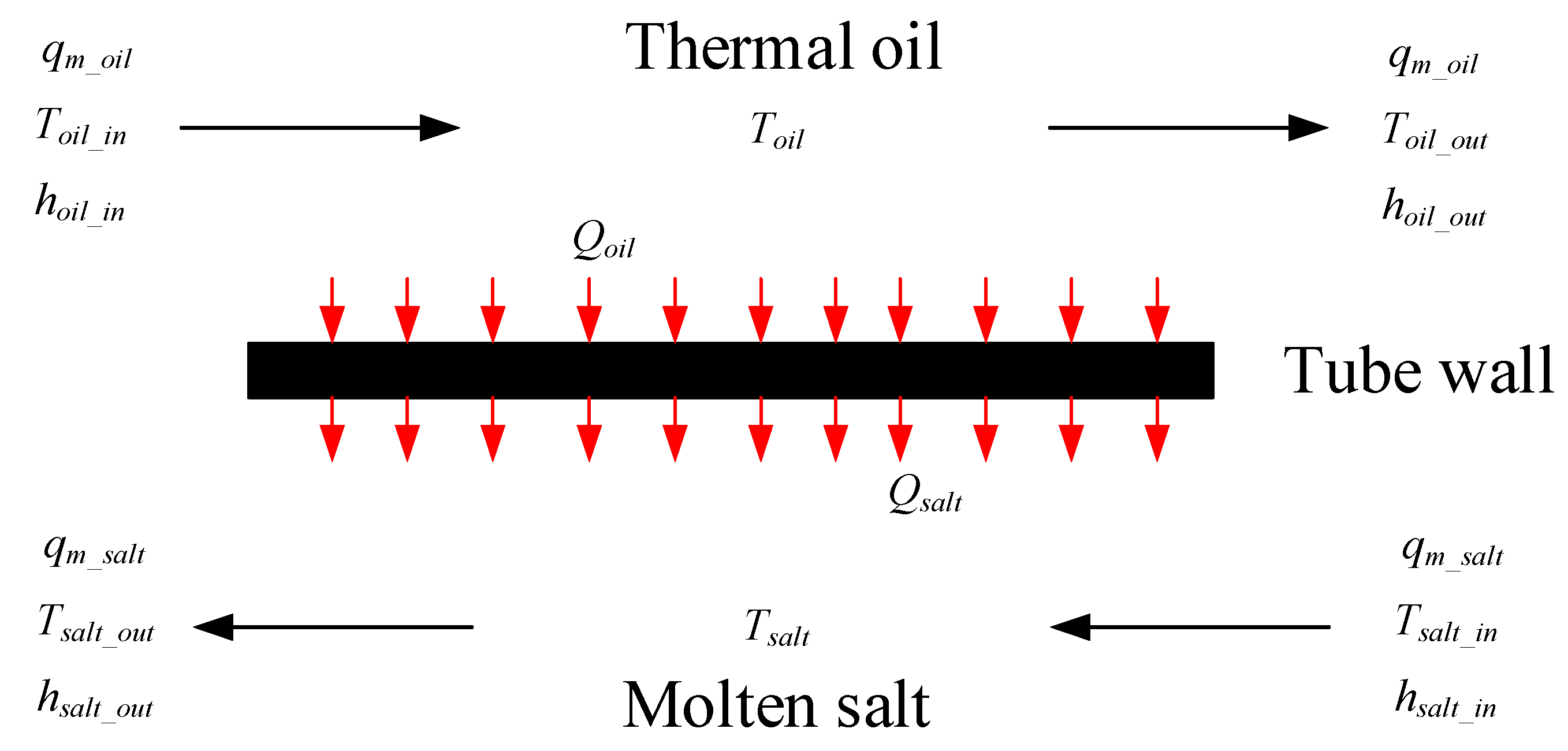
3.3.1. Oil/Salt Heat Exchanger

The oil/salt heat exchanger uses a typical tube and shell heat exchanger. The fluid at the tube side is thermal oil, and the fluid at the shell side is molten salt. The oil/salt heat exchanger model is divided into three parts: the thermal oil side model, the tube wall model, and the molten salt side model. Figure 9 shows the schematic of the oil/salt heat exchanger model.

The thermal oil side model is developed based on energy conservation as follows:

$$\frac{d(c_{p\_oil}{m}_{oil}{T}_{oil})}{dt}=q_{m\_oil}(h_{oil\_in}-h_{oil\_out})-Q_{oil}$$

(44)

The heat released by the thermal oil is calculated by:

$$Q_{oil}=\alpha A_i(T_{oil}-T_{tube})$$

(45)

Here, α is the convective heat transfer coefficient and is calculated by Gnielinski correlation, which is given in Appendix A.

The molten salt side model is developed based on energy conservation as follows:

$$\frac{d(c_{p\_salt}{m}_{salt}{T}_{salt})}{dt}=q_{m\_salt}(h_{salt\_in}-h_{salt\_out})+Q_{salt}$$

(46)

The absorbed heat of the molten salt is computed as:

$$Q_{salt}={\alpha }^{\prime }{A}_o(T_{tube}-T_{salt})$$

(47)

Here, α’ is the convective heat transfer coefficient between the molten salt and tube wall. It is computed by Zhukauskas correlations, which are given in Appendix A.

The tube wall model based on energy conservation is developed as follows:

$$\frac{d(c_{p\_tube}{m}_{tube}{T}_{tube})}{dt}=Q_{oil}-Q_{salt}$$

(48)

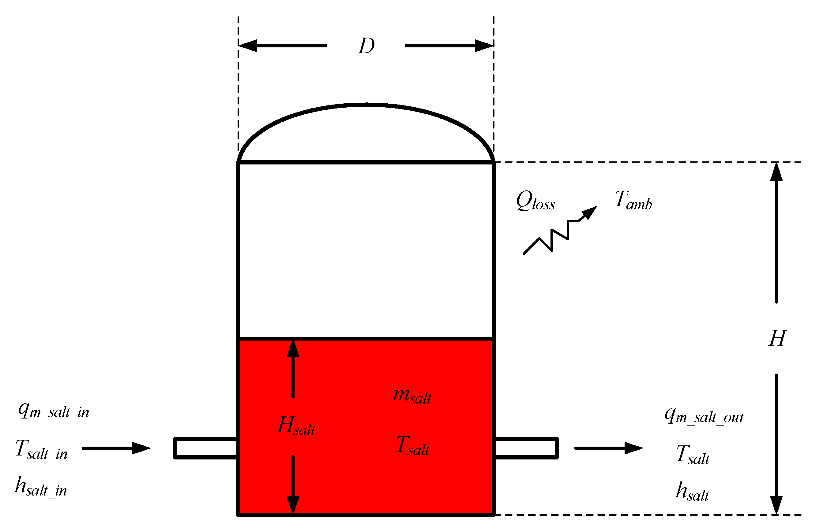
3.3.2. Molten Salt Tank

The molten salt tank is considered as an open system, and its model is developed based on energy conservation. Figure 10 shows the schematic of the model.

The equations used for the model are listed below:

In the molten salt tank, the molten salt temperature is calculated as follows:

$$\frac{d(u_{salt}{m}_{salt})}{dt}=q_{m\_salt\_in}{h}_{salt\_in}-q_{m\_salt\_out}{h}_{salt}-{\alpha }_{tank}{A}_{tank}(T_{salt}-T_{amb})$$

(49)

Here, α_tank is the heat loss coefficient of the molten salt tank, u_salt is the definite internal energy of the molten salt in the tank, m_salt is the molten salt mass in the tank, h_{salt_in} is the definite enthalpy of the molten salt flowing into the tank, h_salt is the definite enthalpy of the molten salt in the tank, and A_tank is the tank’s area, which are calculated by

$$u_{salt}=c_{p\_salt}(T_{salt}-T_{ref})$$

(50)

$$m_{salt}=m_{salt,0}+(q_{m\_salt\_in}-q_{m\_salt\_out})t$$

(51)

$$h_{salt\_in}=c_{p\_salt\_in}(T_{salt\_in}-T_{ref})$$

(52)

$$h_{salt}=c_{p\_salt}(T_{salt}-T_{ref})$$

(53)

$$A_{tank}=\frac{\pi D^2}{4}+\pi DH$$

(54)

In Equation (50), T_ref represents the reference temperature, which is 270 °C. In Equation (51), m_salt,0 represents the initial mass of the molten salt in the tank.

In the tank, the height of the molten salt is calculated by

$$H_{salt}=\frac{4m_{salt}}{{\rho }_{salt}\pi D^2}$$

(55)

3.4. Turbine Generator Model

A turbine generator model turns the output of SGS, namely, temperature, the steam mass flow rate, and pressure, into electrical power. The calculation order of the model is as follows: Firstly, at the inlet of the turbine, the steam entropy and enthalpy can be obtained by the steam temperature and pressure calculated by the SGS model. Then, the steam enthalpy after the isentropic expansion is calculated by the steam entropy and the set steam pressure at turbine outlet. Finally, according to the set efficiency and the steam enthalpy disparity between the outlet and inlet of the turbine, the electrical power is obtained. The equation used for the model is given below:

$$P_{el}={\eta }_{el}{\eta }_t{q}_{m\_steam}(h_{steam\_in}-h_{steam\_out})$$

(56)

Here, η_el is the efficiency of the generator, which is 0.99, η_t is the efficiency of the turbine, which is 0.6, q_{m_steam} is the steam mass flow rate, h_{steam_in} is the definite steam enthalpy at turbine inlet, and h_{steam_out} is the definite steam enthalpy at the turbine outlet. In addition, the steam pressure at the turbine outlet is set to 4.9 kPa.

3.5. Hydraulic Model

The hydraulic model mainly simulates the pressure of every node in the pipe network and the transient features of the mass flow rate on the connecting branch. This includes a pressure node model and a flow model.

The pressure variation of a pressure node in a net flow net can be obtained as follows:

$$\frac{\mathrm{d}m}{\mathrm{d}t}=\frac{\mathrm{d}(\rho V)}{\mathrm{d}t}=V\frac{\mathrm{d}\rho }{\mathrm{d}t}=V(\frac{\partial \rho }{\partial p}\frac{dp}{dt}+\frac{\partial \rho }{\partial T}\frac{dT}{dt})=q_{\mathrm{m}\_\mathrm{in}}-q_{\mathrm{m}\_\mathrm{out}}$$

(57)

Considering the pressure variation rate is faster than that of the temperature due to thermal inertia, Equation (57) is transformed as:

$$\frac{dp}{dt}=\frac{q_{\mathrm{m}\_\mathrm{in}}-q_{\mathrm{m}\_\mathrm{out}}}{V\frac{\partial \rho }{\partial p}}=\frac{(q_{\mathrm{m}\_\mathrm{in}}-q_{\mathrm{m}\_\mathrm{out}})}{c^{″}}$$

(58)

where c” is the fluid compressibility coefficient.

The mass flow rates are determined by the pressure difference, and the correlation is given in Appendix B.

3.6. Working Fluid Properties

In this study, the variations of the working fluid properties with temperature are considered. The thermal oil used in the Yanqing plant is Therminol-VP1, and its molten salt is a kind of Solar salt (60% NaNO₃ and 40% KNO₃ by weight percent). Their properties are given in Appendix B.

The water/steam properties are obtained by IAPWS-IF97 [30]. The relevant calculation was coded.

4. Modeling Validation

4.1. SF

The SCA model is compared with the model developed by Jeter [31,32]. The comparison results show good agreement, which verifies the accuracy of the model. Detailed comparison results are provided in reference [33].

The receiver model is verified by the experimental data. The data are obtained by two different dynamic conditions, which are Case 1 (cloudy for a long time) and Case 2 (cloudy for a short time). The comparison results are shown in Figure 11.

In Case 1, at t = 11:16, the DNI suddenly decreased to zero, and the thermal oil temperature began to drop. In Figure 11a, the simulated temperatures of the thermal oil at the outlet are consistent with that of the measured results with both its maximum values occurring at the same time. The maximum error is 11.4 °C because of the low mirror cleanliness and reflectance due to dust and other experimental conditions. However, in the simulation, the theoretical mirror cleanliness and reflectance are adopted, which provided better results. When the DNI value dropped to 0, the simulated and measured values agreed well.

As shown in Figure 11b, in Case 2, the simulation results of the outlet thermal oil temperature match well with that of the measured results. The overall DNI variation was stable. At 12:45, the DNI shortly decreased due to the cloud cover but increased soon after. With the increase of the thermal oil temperature at the inlet, the simulation results and measured results of the outlet temperature both increased, with their variation trends agreeing well.

The simulation results showed a pleasant correspondence with the experiment data in the dynamic processes, which proves that the model can be used in the analysis of the dynamic characteristics of the system.

4.2. SGS

We compared the simulation values of the cricital SGS system parameters under design operation conditions with the design values to validate the SGS model. The validation results are shown in

Table 4. Validation results.

	Preheater		Evaporator			Superheater
	Oil Outlet Temperature	Water Outlet Temperature	Oil Outlet Temperature	Steam Outlet Temperature	Steam Outlet Pressure	Oil Outlet Temperature	Steam Outlet Temperature
Design values	296 °C	230 °C	317.9 °C	235.1 °C	3.12 MPa	379.9 °C	383 °C
Simulation values	296.0 °C	231.7 °C	315.7 °C	236.0 °C	3.12 MPa	379.7 °C	383.4 °C
Relative errors	0%	0.74%	0.69%	0.38%	0%	0.05%	0.10%

. The simulation values match well with the design values. The maximum error is only 0.74%, which verifies the SGS model.

4.3. Two-Tank Indirect TES System

To verify the accuracy of the oil/salt heat exchanger model in dynamic working conditions, the developed model was compared with that of Zaversky [34], which has been validated under multiple working conditions. The Zaversky model is used as the reference model to verify the oil/salt heat exchanger model under four dynamic conditions: Case 1: thermal oil flow disturbance under rated conditions; Case 2: thermal oil flow disturbance under 50% rated conditions; Case 3: thermal oil inlet temperature disturbance under rated conditions; and Case 4: thermal oil inlet temperature disturbance under 50% rated conditions. The dynamic working conditions are defined in

Table 5. Dynamic working conditions.

Index	Thermal Oil Inlet Temperature (°C)	Molten Salt Inlet Temperature (°C)	Thermal Oil Mass Flow Rate (kg/s)	Molten Salt Mass Flow Rate (kg/s)
1	391	292	600 until t = 2500 s 300 until t = 5000 s 600 remaining time	899
2	391	292	300 until t = 3500 s 150 until t = 7000 s 300 remaining time	470
3	391 until t = 2500 s 371 until t = 5000 s 391 remaining time	292	600	899
4	391 until t = 3500 s 371 until t = 7000 s 391 remaining time	292	300	470

. The comparison results are shown in Figure 12. In Figure 12, LPM is short for lumped parameter model, representing the oil/salt heat exchanger model developed in this paper.

Figure 12 indicates the excellent agreement of the simulation results of the two models under the four dynamic processes, which verifies the accuracy of the developed oil/salt heat exchanger model in this study.

When validating the molten salt tank model, the calculation results of the System Advisor Model (SAM) software are used in this study. SAM is free software developed by NREL, which can simulate the performance of solar thermal power generation system. At present, researchers have used the SAM software in analyzing the system performance of the PTSP plant [35]. In addition, it is also used to test Andasol I trough power station in Spain. Using open limited data information, the error between the simulation results and reported annual power generation is only 2.6% [36], which verifies the reliability of the software.

In this study, three different working conditions were compared and verified: Case 1: no standby condition of the heat storage system in clear weather, Case 2: standby condition of the heat storage system in clear weather, and Case 3: cloudy weather. In the calculation, the model of molten salt tank is set up with the same initial parameters and entry boundary conditions as the SAM software. The entry boundary conditions include the flow rate and temperature of the molten salt as well as the environmental temperature. The initial parameters include the temperature and volume of the molten salt at the initial time to obtain the temperature changes and the molten salt volume in the tank at other times. Because the output of the SAM software is only the molten salt volume in the tank and there is no height involved, the volume of the molten salt is used in this study.

The comparison and verification results in different working conditions are shown in Figure 13. The results of the temperature and the molten salt volume in the tank calculated by the model agreed well with those obtained by SAM. This proves that the developed molten salt tank in this paper can be useful in the analysis of the system dynamic features. In Figure 13, LPM is short for lumped parameter model, representing the molten salt tank model developed in this paper.

5. Models Integration on the STAR-90 Simulation Platform

The developed models were integrated into the simulation platform of STAR-90 to conduct systematic simulations. As a real-time simulation platform, STAR-90 has been applied in the analysis of the dynamic features of CSP plants [28]. Figure 14 shows the final effect of the models integrated on the STAR-90 platform. Apart from the SF, two-tank indirect TES system, and SGS models, existing models in the library, including valves, pumps, a buffer tank, and control modules, are also utilized.

6. Control and Operation Strategies

Because DNI varies on a clear or cloudy day, the steam parameters generated by SGS accordingly change in a PTSP plant. This instability of the steam parameters harms the operation of the turbine. Hence, the objective of the control and operation strategies for the dynamically coupled operation is to produce the SGS output as smoothly as possible with the help of the TES system. In this study, for practical purpose, the real meteorological data on a clear day and a cloudy day in Yanqing is chosen to conduct system-level simulations. The actual meteorological data are obtained by a weather station in Yanqing shown in Figure 15.

The control strategies used for the coupled operation are shown in Figure 16. As shown in Figure 16a, the water level is adjusted to 0.8 m using the PI controller which regulates the feed water mass flow rate. The thermal oil temperature at the outlet of SF is maintained at 393 °C using a PI controller which regulates the thermal oil mass flow rate. Figure 16b shows the control strategies used for the TES system. During the charge process, the controlling valve at the thermal oil inlet of the oil/salt heat exchanger adjusts the surplus thermal oil mass flow rate into the TES system using the PI controller to hold the thermal oil mass flow rate in the power block at 30,000 kg/h. The controlling valve at the molten salt inlet adjusts the molten salt mass flow rate using the PI controller to hold the molten salt outlet temperature at 386 °C. During the discharge process, the controlling valve at the thermal oil inlet of the oil/salt heat exchanger supplements the mass flow rate of thermal oil into the TES system using the PI controller to hold the mass flow rate of the thermal oil running through the power block at 30,000 kg/h. The controlling valve at the molten salt inlet adjusts the molten salt mass flow rate using the PI controller to hold the thermal oil outlet temperature at 378 °C.

Different operation strategies are used on a clear and cloudy day, which are introduced in the following parts.

6.1. On a Clear Day

The meteorological data on a clear day at the Yanqing plant are obtained on 20 September 2017. The data include wind speed, DNI variations, and environmental temperature on this day as shown in Figure 17. Figure 17 shows that the DNI change with time is steady and it has a maximum value, which is 902.7 W/m², at around 12:00. On the other hand, the ambient temperature reached its peak value of 25 °C at about 14:00. The wind speed ranged from 0.1 m/s to 4.4 m/s. The daytime on this day was nearly 12 h.

The operation strategy is shown in Figure 18. At the beginning of the system operation, the thermal oil first recirculates along Circuit 1 in SF at a minimum mass flow rate of 3583 kg/h in this case until its temperature at the SGS inlet reaches the minimum temperature of 310 °C [10]. Then, the valve at the thermal oil inlet of the SGS on Circuit 2 opens and thermal oil starts to flow through SGS. When the thermal oil mass flow rate in the power block reaches 30,000 kg/h, the valve at the thermal oil inlet of the TES system on Circuit 3 opens, and the charge process starts. In the power block, when the thermal oil mass flow rate is less than 30,000 kg/h, the thermal oil in the TES system starts to flow reversely, and the discharge process starts. During the discharge process, the thermal oil mass flow rate in the TES system is adjusted to maintain it to 30,000 kg/h in the power block. When the height of molten salt in the hot tank is less than 0.5 m, the discharge process stops. Then, the thermal oil continues to recirculate along Circuit 1. This ends the operation on a clear day.

6.2. On a Cloudy Day

The meteorological data of a cloudy day were obtained on 26 March 2017, as shown in Figure 19. As seen in Figure 19, the DNI showed vibrations with its maximum value of 878.2 W/m². The wind speed also showed oscillation with its maximum value of 7.8 m/s and a minimum value of 0.9 m/s. The ambient temperature increased from −0.9 °C and reaches the maximum value of 9 °C at 14:00. From then on, the ambient temperature began to decrease.

On a cloudy day, there is a sudden reduction of DNI, which increases the number of start-up and close-down events in the power block. To avoid damages from frequent start-ups and stops, based on the concept described by Astolfi et al. [37], the TES system is operated before the SGS. The operation strategy on a cloudy day is shown in Figure 20. At the beginning of the system operation, the charge process starts first. When the thermal oil outlet temperature in the SF is less than 390 °C, the discharge process starts. When the molten salt height in the hot tank decreases to 0.5 m, the discharge process stops. Then, the thermal oil continues to recirculate along Circuit 1. This ends the operation on a cloudy day.

7. Results and Discussions

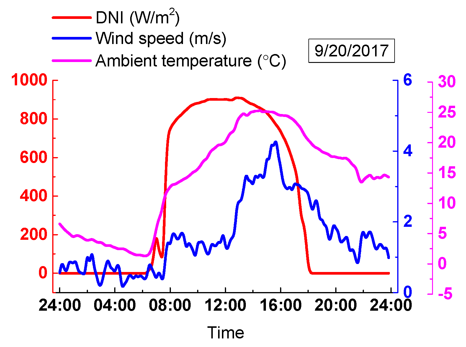
Because the interval of the measured meteorological data is 10 min and the running step of the dynamic simulation program is 0.5 s, the linear interpolation method is used in the simulation process to match them. The initial parameters for the system-level simulations on a clear day and cloudy day is given as follows: in the case of the clear day, the initial thermal oil inlet and outlet temperature in SF were set to 120 °C and 230 °C, respectively. The feed water temperature was adjusted to 104 °C and kept constant. The initial steam pressure and mass flow rate were set to 0.1 MPa and 0 kg/s, respectively. In the evaporator, the initial water height was adjusted to 0.678 m. The initial molten salt temperature and height in the hot tank were set to 300 °C and 0.1 m, respectively. The initial temperature and height of molten salt in the cold tank were set to 292 °C and 3.5 m, respectively. In the case of the cloudy day, the initial conditions for the simulation were the same as those on a clear day except the initial height of the molten salt in the cold tank, which is 6 m.

The dynamic behavior of SF, SGS, and two-tank indirect TES system is described in the following parts.

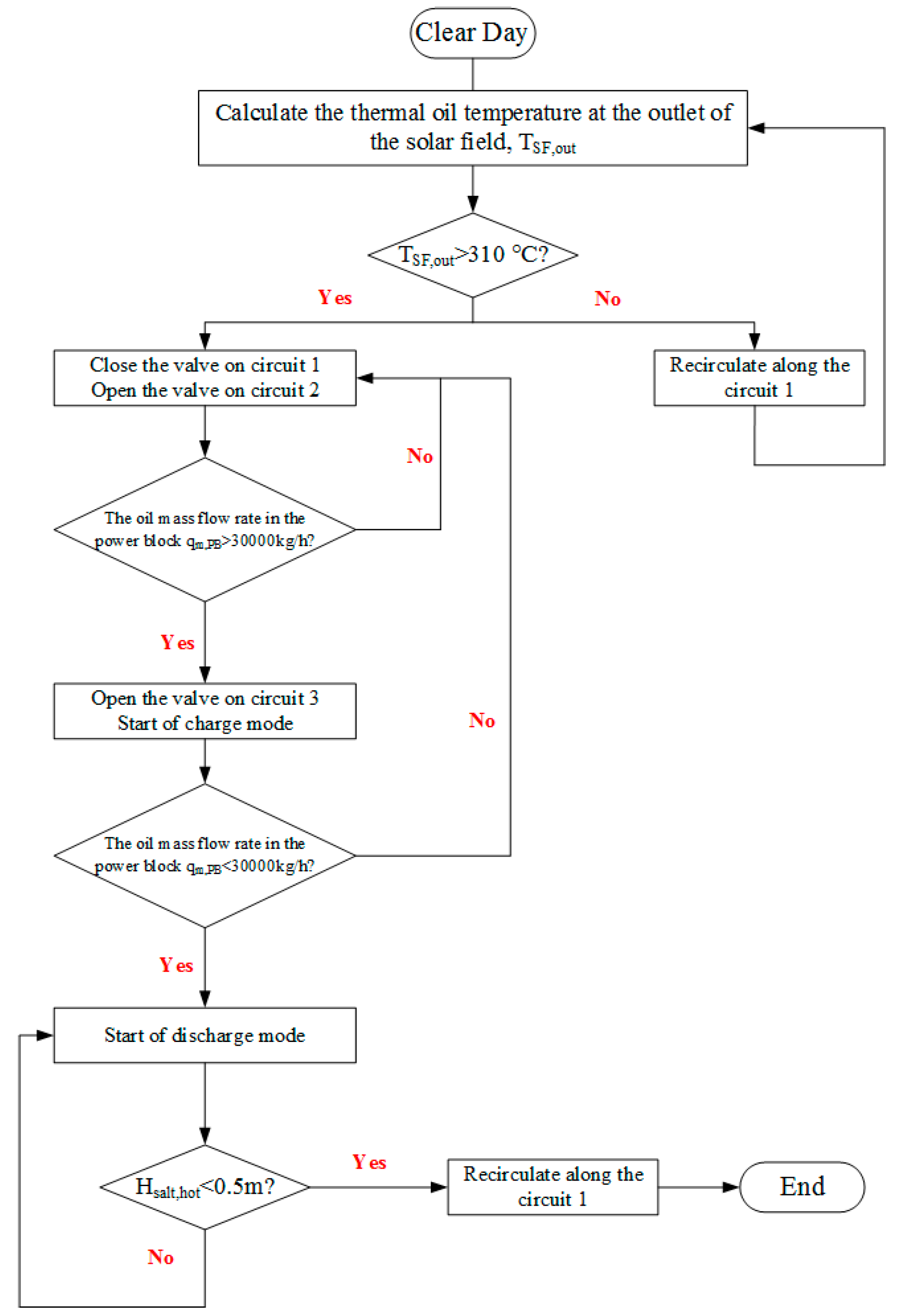
7.1. On a Clear Day

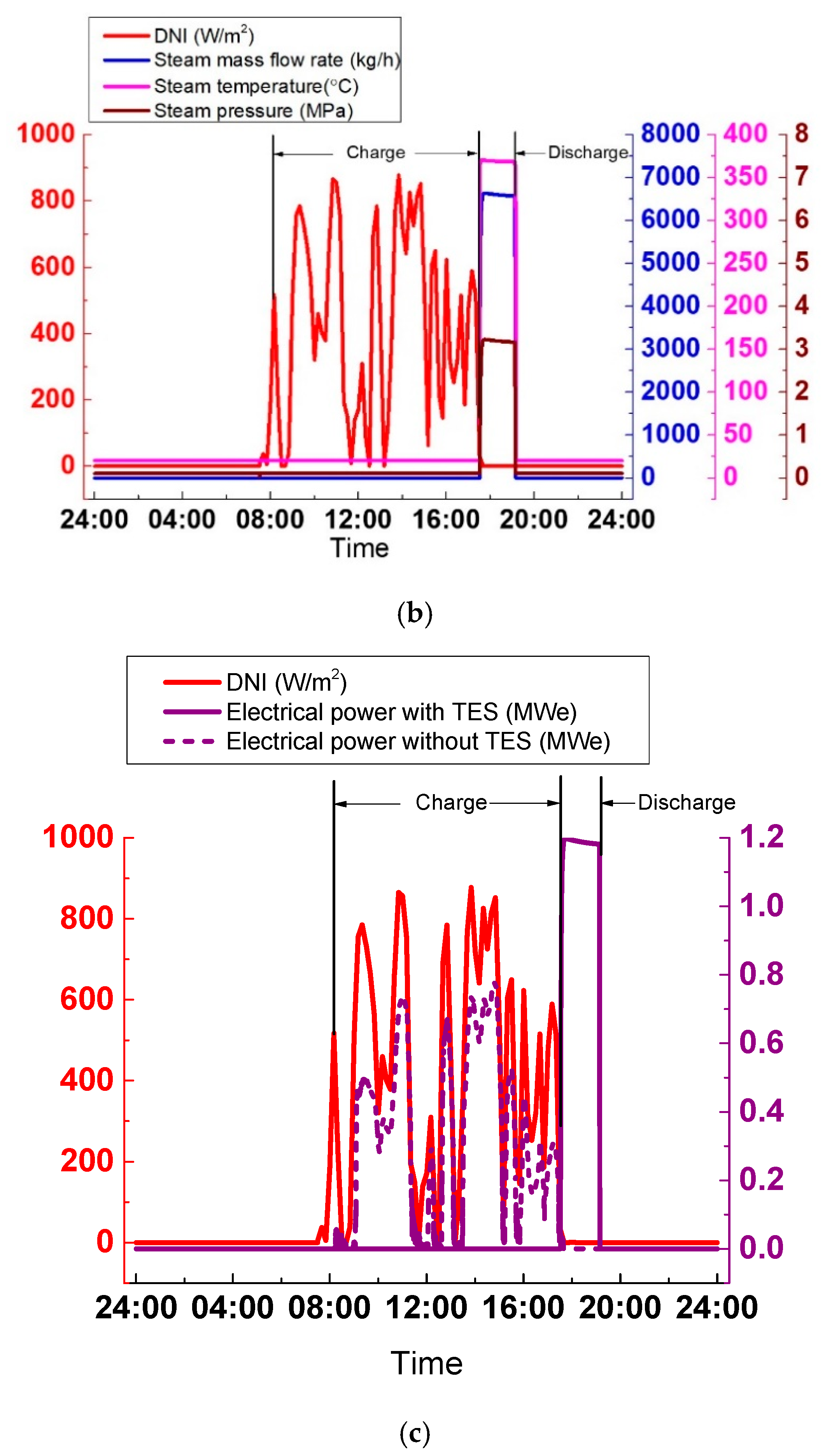
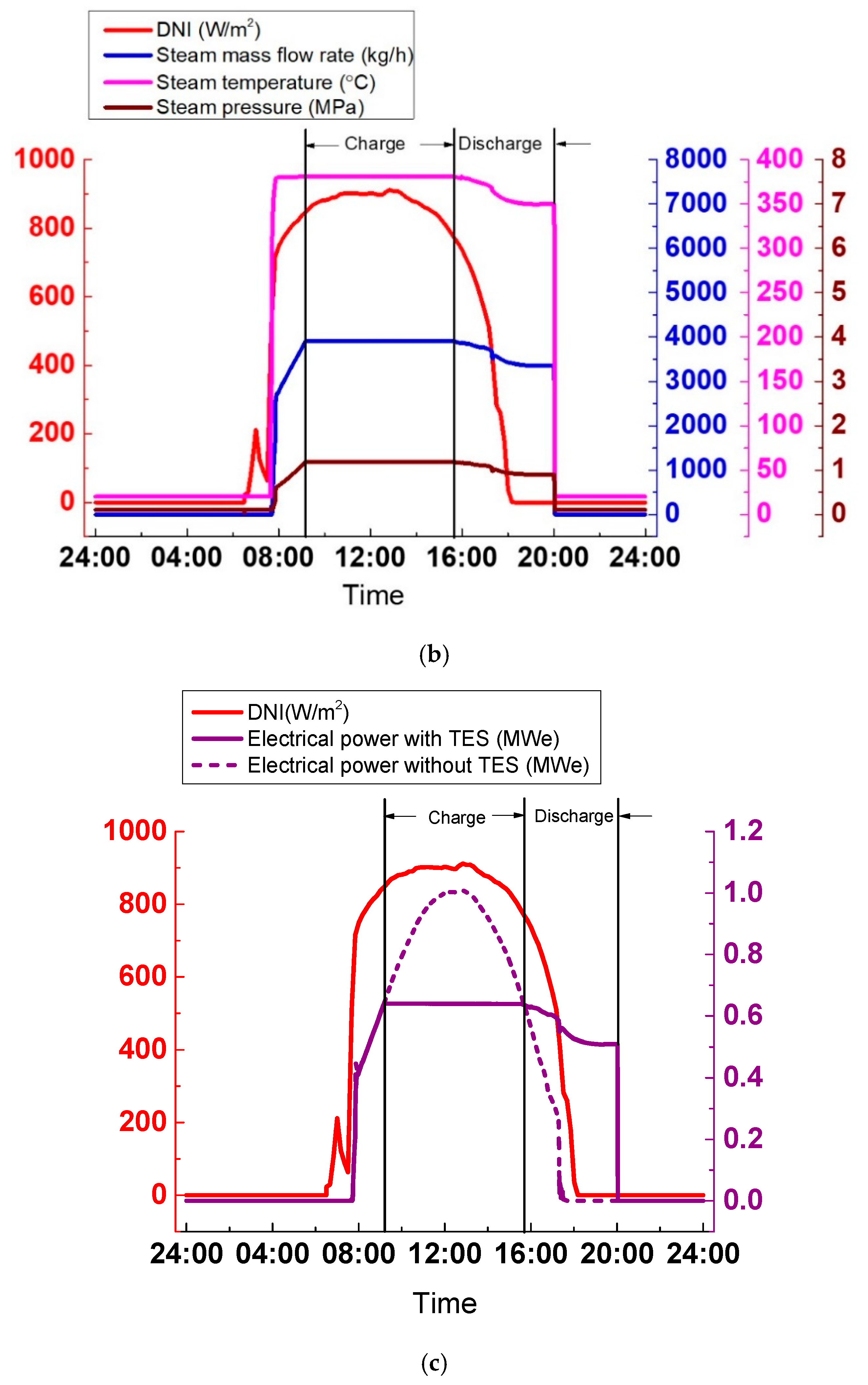
As shown in Figure 21b, the SGS output, namely, temperature, pressure, and steam mass flow rate, is smoothened with the TES system. The charge process lasts from 9:07 to 15:34 and the discharge process follows and ends at 20:00. During the charge process, the steam parameters remain stable, which are 3913 kg/h, 381 °C, and 1.19 MPa. At the beginning of the discharge process, the steam parameters slowly decrease; the steam temperature from 381–354 °C in 2.5 h and the steam pressure from 1.19–0.94 MPa, which leads to a drop of 480 kg/h in the steam mass flow rate. This is attributed to the slow drop of the thermal oil temperature at the SGS inlet. The thermal oil at the SGS inlet is from the mixture of the thermal oil at the outlets of the SF and TES system. The thermal oil temperature at SF outlet decreases from 393–201 °C due to the decrease of the solar radiation, but the thermal oil outlet temperature in the TES system keeps constant at 378 °C; hence, the thermal oil temperature at the inlet of SGS decreases. When the temperature of thermal oil outlet in SF tends to be constant at t = 19:24, the thermal oil inlet temperature in SGS also tends to be constant at 358 °C. Therefore, the SGS output is smoothened again, as shown in Figure 21b. Meanwhile, in comparison with the SGS output without the TES system as shown in Figure 21a, the TES system shifts from the peak time of solar radiation to that of the electricity demand. It also extends the generation period for 2.5 h. This is illustrated better in Figure 21c. During the charge process, the electrical power keeps stable at 0.64 MWe. At the beginning of the discharge process, electrical power decreases from 0.64 MWe to 0.5 MWe. And then, the electrical power remains nearly constant until the discharge process ends. The total generation period is now from 7:44 to 20:00.

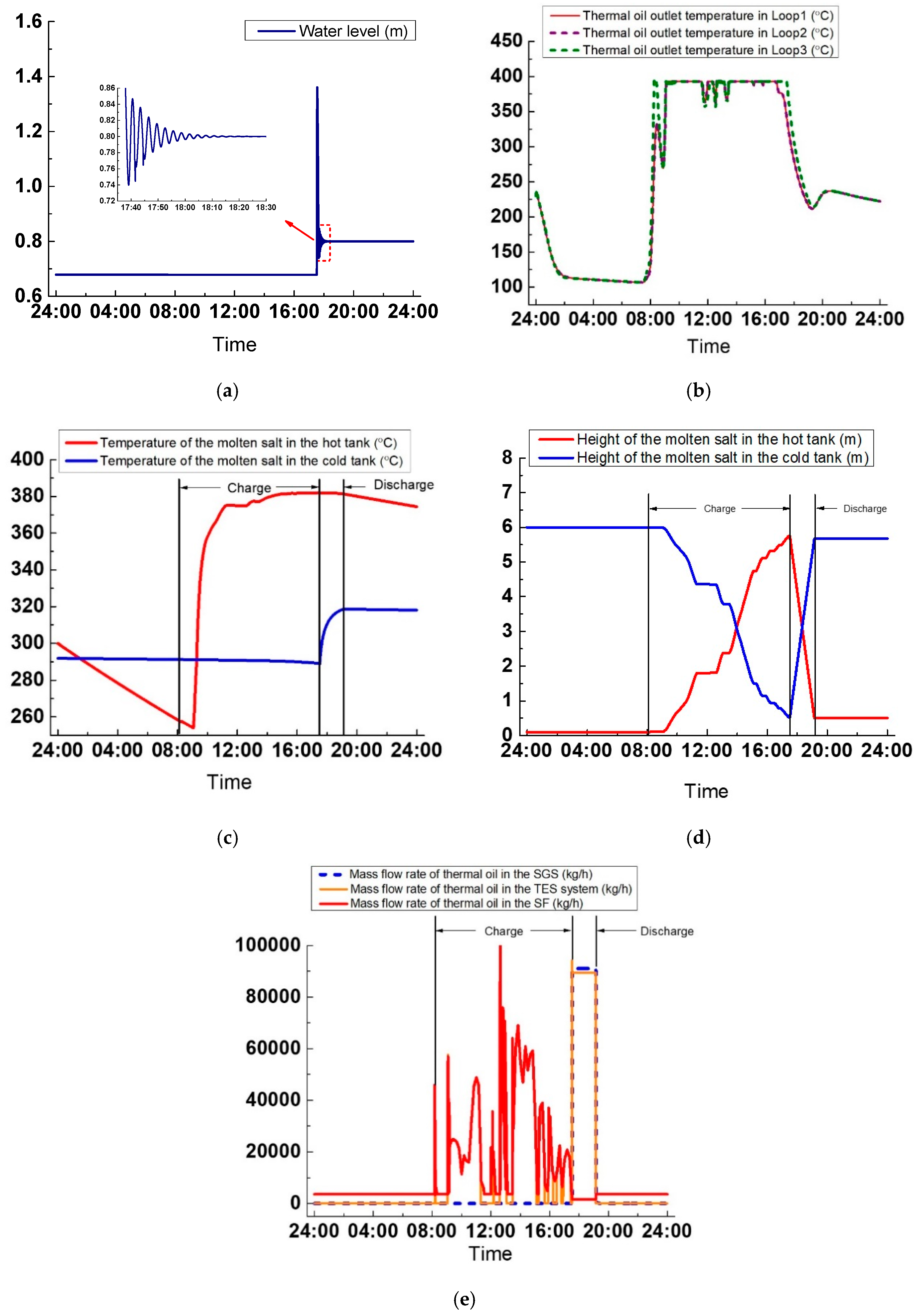
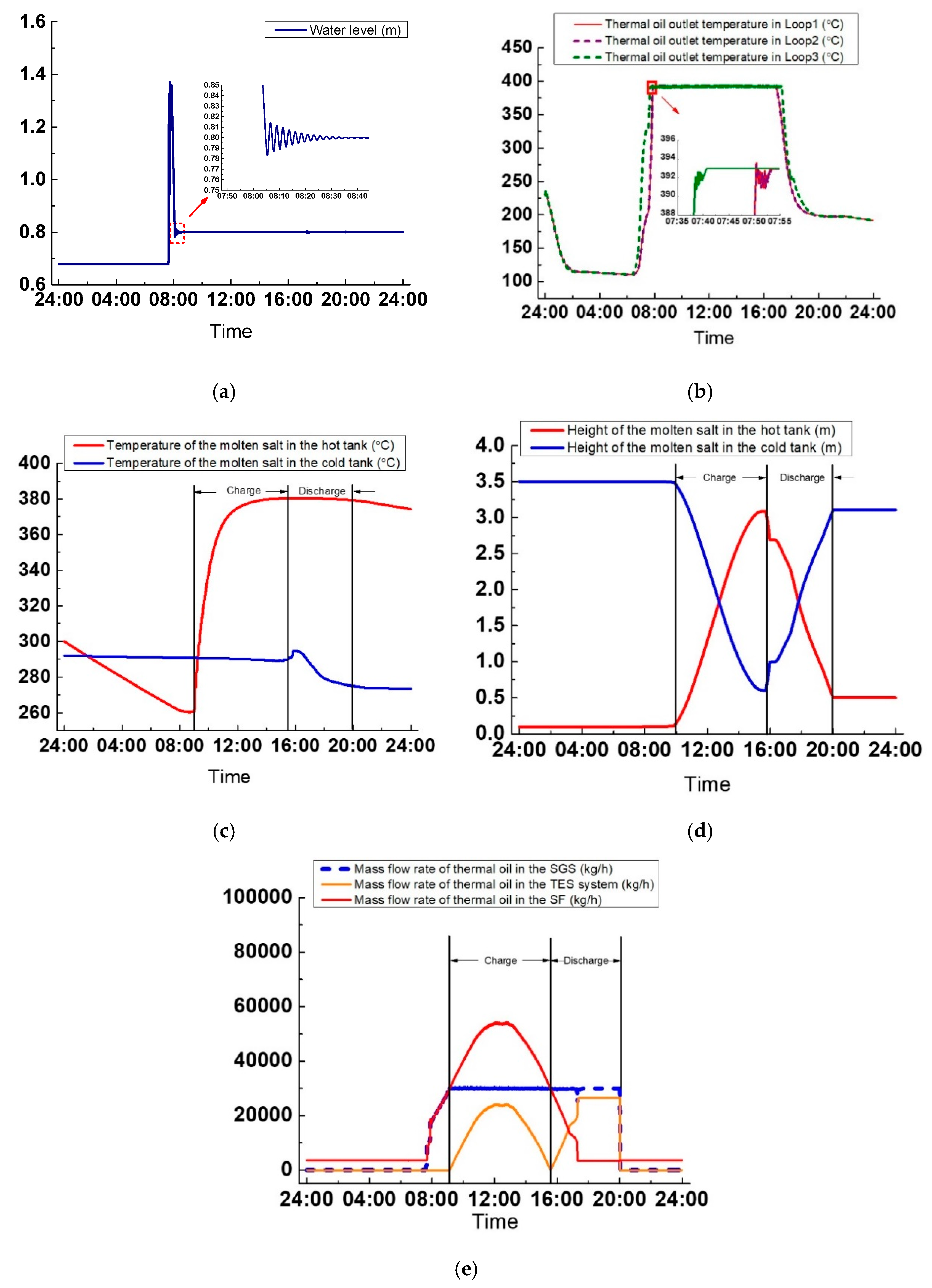
As seen in Figure 22a, the control effect of the water level is good. The maximum deviation is only 10 mm (the water level’s first peak is mainly related to the initial parameters instead of the control strategy). The transition time lasts nearly 1 h, from 7:44 to 8:40. Figure 22b indicates the variations of the thermal oil outlet temperature in the three loops. From t = 0:00 to t = 2:00, the thermal oil temperatures at three loops’ outlets all decrease from 230 °C to 115 °C because DNI is zero. From t = 2:00 to 6:17, SF is under heat balance, and the thermal oil temperature at the outlets stay nearly constant at around 112 °C. When DNI is above zero at t = 6:30, the thermal oil temperature starts to increase. The thermal oil outlet temperature in Loop 3 increases faster than that at the outlets of Loop 1 and 2 because of the different layouts. The thermal oil outlet temperature in Loop 3 reaches approximately 393 °C at t = 7:39, and the PI control then starts to run. The thermal oil temperature at the outlets of Loop 1 and 2 reaches 393 °C at t = 7:51 and the PI control then begins to adjust it. In Figure 22b, the thermal oil outlet temperature in the three loops is controlled well at 393 °C from 7:55 to 16:47. At 16:47, the thermal oil outlet temperatures in Loop 1 and Loop 2 begin to drop because of the very low DNI and the thermal oil outlet temperature in Loop 3 starts to decrease at t = 17:17.

As shown in Figure 22c, before the charge process, the molten salt temperature in the hot tank decreases from 300–261 °C due to the heat loss to the ambient air, but the molten salt temperature in the cold tank only decreases by 1 °C, from 292–291 °C, because the cold tank stores more molten salt than the hot tank. During the charge process, the temperature of molten salt in the hot tank increases gradually and reaches 380 °C. In the discharge process, the molten salt temperature in the cold salt tank rises first and then drops to 275 °C because of the inconsistent molten salt temperature at the outlet of the oil/salt heat exchanger. The molten salt temperature in the hot tank decreases slightly, from 380–379 °C in 4.5 h, because the hot tank has more molten salt after the charge process.

In Figure 22d, during the charge process, the variation rate of the molten salt height in both tanks first increases from 0.0072–0.72 m/h and then decreases to 0.0072 m/h again. This is attributed to the increase and decrease in the thermal oil mass flow rate in the TES system during the charge process. Hence, to maintain the molten salt temperature at the outlet of the oil/salt heat exchanger, the molten salt mass flow rate in the TES system also increases initially and decreases afterward. During the discharge process from t = 15:57 until t = 16:22, the variation of the molten salt height in the tank is not identical to that of other periods due to the PI control for the working fluid temperature at the outlet of the oil/salt heat exchanger. In Figure 22d, when the charge process ends, the molten salt height in the cold tank is 0.603 m, above the minimum height 0.5 m, which means that some molten salts are not used in the charge process. For this case, when the thermal oil mass flow rate in the SGS is set to 30,000 kg/h, the optimum molten salt storage mass should be 155,981 kg.

In Figure 22e, the thermal oil mass flow rates in TES system, SGS, and SF are presented. As illustrated in Figure 22e, the PI controller adjusts the thermal oil mass flow rate well. At t = 7:39, the thermal oil starts to flow into the SGS with its equal to that in the SF. At t = 9:07, the charge process starts, the thermal oil starts to flow into the SGS and TES system simultaneously. The thermal oil mass flow rate in SGS is maintained at 30,000 kg/h. The mass flow rate of the thermal oil flowing though SF is equal to the sum of thermal oil mass flow rate in SGS and the TES system. During the discharge process, the mass flow rate of thermal oil in SGS is equivalent to the amount of the mass flow rate of thermal oil in the TES system and SF. When the discharge process ends, the thermal oil recirculates again with its mass flow rate kept to a minimum of 3583 kg/h.

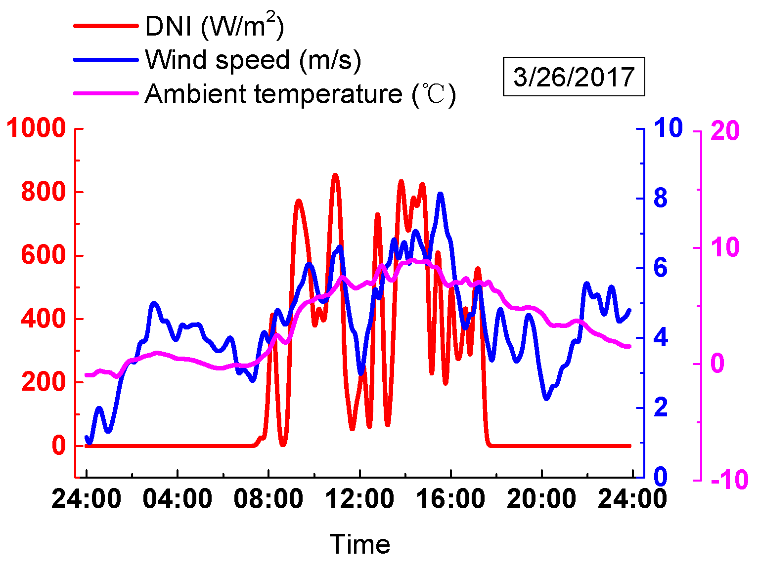
7.2. On a Cloudy Day

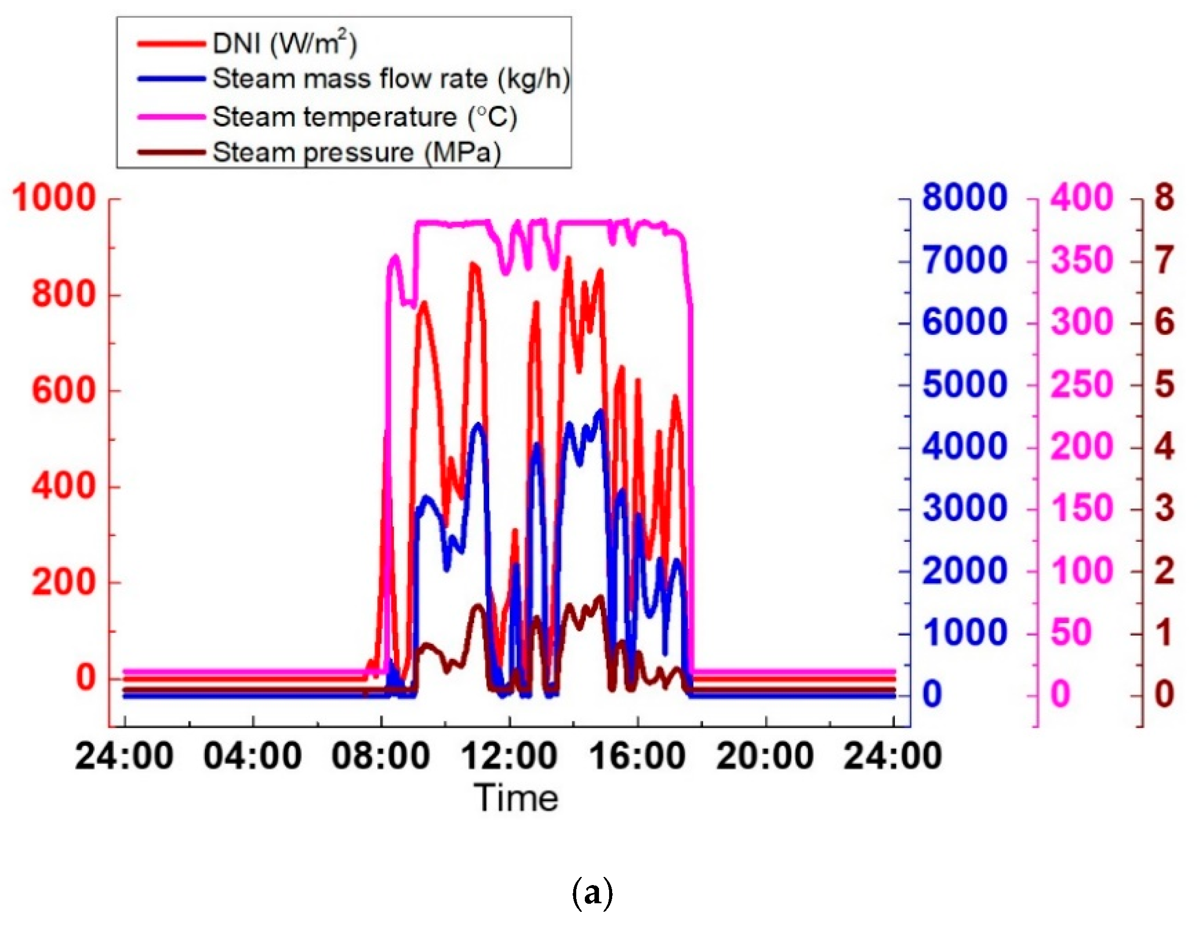
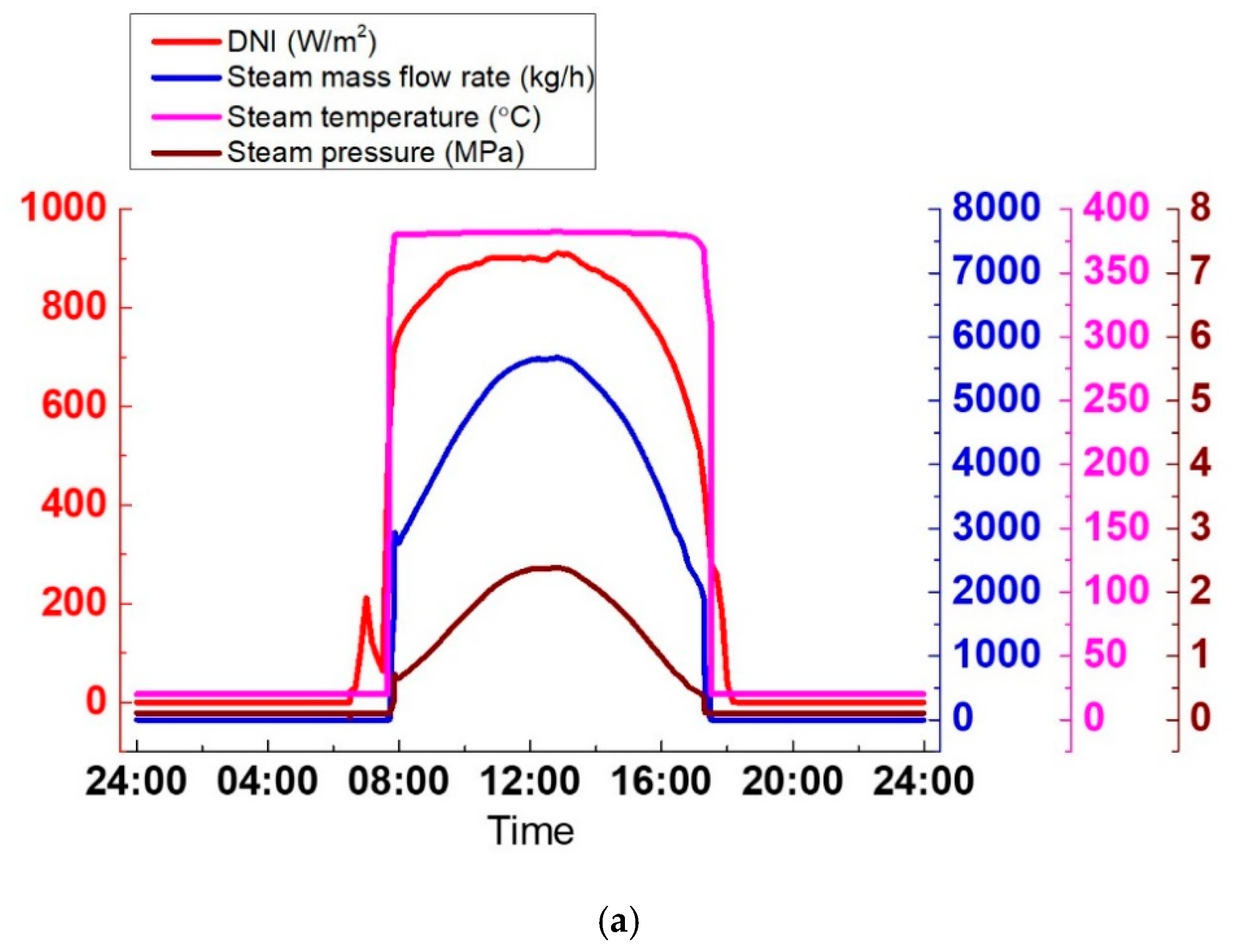
As shown in Figure 23a, the steam parameters generated by the SGS vary widely due to the extreme variations of DNI, which is harmful for the steam turbine operation. Hence, it is necessary to avoid the periods when DNI strongly varies. In Figure 23b, with the TES system, the cloudy condition is avoided, and the SGS output is kept stable. During the discharge process, temperature, pressure, and the steam mass flow rate are 370 °C, 3.2 MPa, and 6600 kg/h, respectively. The SGS output can be adjusted according to the grid by altering its thermal oil mass flow rate. The discharge process lasts approximately 1.5 h, from 17:31 to 19:09. The advantage of the TES system can be explained more clearly in Figure 23c. The electrical power varies widely without the TES system. By contrast, with the TES system, the electrical power remains constant at 1.19 MWe.

As seen in Figure 24a, the control effect of the water level is good. The maximum deviation is 50 mm (the earliest peak of the water level is chiefly related to the initial parameters instead of the control strategies). The transition time lasts about 1 h, from 17:35 to 18:30. In Figure 24b, the variations of the thermal oil temperature at three loops’ outlets are shown. Before the sun rises, the variations of the thermal oil outlet temperature in three loops are similar to those on a clear day. From t = 0:00 to t = 3:00, the thermal oil temperature at the outlets all declines from 230–112 °C, and from t = 3:00 to 7:22, the thermal oil temperature at the outlets keeps nearly constant at around 110 °C. The temperature starts to increase at t = 7:30 when DNI is above zero. The temperature is not kept constant during the operation. This is due to the cloudy day in which the DNI varies and reaches a lower value that cannot ensure a steady thermal oil temperature at the minimum thermal oil mass flow rate. However, the temperature of the thermal oil outlet is mostly controlled at 393 °C.

In Figure 24c, from t = 0:00 to t = 8:14, the molten salt temperature in the hot tank declines from 300–257 °C, and the temperature of molten salt in the cold tank decreases from 292–291 °C. During the first 48 min of the charge process, the temperature of molten salt in the hot tank still decreases because the energy absorbed by the tank cannot eliminate the heat loss. Then from t = 9:04, the temperature of molten salt in the hot tank increases gradually and reaches 382 °C. However, the temperature variation is not constant because of the variations of the molten salt temperature at the outlet of the oil/salt heat exchanger. During the discharge process, the temperature of molten salt in the cold salt tank rises to 313 °C because the oil/salt heat exchanger is not working under its rated condition. The temperature of molten salt at the heat exchanger outlet is 315 °C, which is more than the initial temperature of 292 °C in the cold tank; hence, the temperature of molten salt in the cold salt tank increases. The temperature of molten salt in the hot tank keeps nearly constant at 382 °C. After the discharge process ends, from t = 19:09 to t = 24:00, the molten salt temperature in the hot and cold tanks both drops slightly. For the hot tank, the temperature drop is 7 °C; and for the cold tank, it is 0.6 °C.

In Figure 24d, during the charge process, the variation of the molten salt height in either tanks is not smooth. This is caused by the molten salt mass flow rate in the TES system, which varies with the thermal oil in the SF to maintain the molten salt temperature at the outlet of the oil/salt heat exchanger. The variation of the thermal oil mass flow rate in SF is rough because of the substantial variations of the DNI, as shown in Figure 24e. During the discharge process, because the molten salt mass flow rate is kept constant, the variation speed of the molten salt height is maintained at 3.6 m/h. By comparing the different variations of the molten salt height during the charge and discharge processes, it can be concluded that mass flow rate of the molten salt flowing in or out the tank affects the molten salt height more than the physical property of the molten salt. It can also be seen from Figure 24d that after the charge process is over, the height of the molten salt in the cold tank is 0.528 m, higher than the minimum height of 0.5 m, which indicates that excessive molten salt is used. For this case, the optimum molten salt storage mass should be 294,626 kg, which is more than the optimum mass on the clear day.

Figure 24e shows that during the charge process, the thermal oil mass flow rate in SF varies more frequently than that on a clear day because of the wide DNI variations on a cloudy day, which varies the thermal oil mass flow rate under the action of the PI controller to maintain the temperature of the thermal oil outlet in SF. During the discharge process, the thermal oil mass flow rate in SGS is kept unchanged at 91,044 kg/h. When the discharge process ends, the thermal oil recirculates again at a minimum mass flow rate of 3583 kg/h.

8. Conclusions and Future Research

In this study, SGS and the two-tank indirect TES system in the Yanqing pilot plant were used to study the dynamically coupled operation of these two systems. System simulations on a clear day and a cloudy day were carried out to study the influence of the two-tank indirect TES system on the dynamic characteristics of SGS. Meanwhile, the control and operation strategies were also presented. The conclusions are obtained as follows:

• With the TES system, the SGS output was smoothened and the generation period was extended.
• During the transition time from the charge to the discharge process, the steam parameters were slowly decreased.
• The molten salt mass flow rate flowing in or out of the tank affected the molten salt height more than the molten salt’s physical properties.
• PI control can be applied for the adjustments of the thermal oil mass flow rate, thermal oil temperature, and water level in a PTSP plant.

The modeling methods described in this study can be used in developing a simulator for a PTSP plant to obtain a suitable control strategy for plant operation. In the future, based on the models developed in this paper, the effect of three different molten salts (Hitec, a ternary mixture of KNO₃, NaNO₂ and NaNO₃; Hitec XL, a ternary mixture of KNO₃, NaNO₃, and Ca(NO₃)₂; Solar salt, in this paper) on the operation of the system will be studied and the parameter analysis of the relationship between the optimum molten salt storage mass and the system power generation will be conducted in detail.