Research on Improved Auto-Tuning of a PID Controller Based on Phase Angle Margin

Abstract

In order to realize fast and efficient tuning of the proportional-integral-derivative (PID) controller parameters in thermal power plants, this paper thoroughly analyzes the problems existing in the relay characteristic method based on the phase angle margin auto-tuning method (PM method), and proposes an improved PM auto-tuning method for the most common first order plus dead time (FOPDT) model in practical engineering applications. The improved algorithm proposes the design of the target phase angle margin and the method of plant identification. Then, the optimization algorithm is used to calculate the correction coefficient of the setting formula to obtain the PID controller parameters that minimize the integrated time absolute error (ITAE) index of the control system. Finally, through the auto-tuning experiment on the generalized control model of the main steam temperature system in thermal power plants, it is verified that the improved algorithm is superior to the traditional PM method and Ziegler–Nichols method (Z-N method), and can obtain a fast and stable control performance.

1. Introduction

The proportional-integral-derivative (PID) controller is widely used in industry with the characteristics of a simple structure and strong robustness [1]. In thermodynamic systems, the characteristic parameters of each thermal plant often change in different operation conditions, so the fixed controller parameters cannot always meet the control requirements [2]. The fast self-tuning PID algorithm can adjust parameters of controllers online according to the characteristics of the controlled plant, maintaining the stability, rapidity and robustness of the control system. In thermal power plants, process plants usually exhibit first order plus dead time (FOPDT) characteristics, while larger delay times increase the difficulty of self-tuning control.

Ziegler and Nichols first proposed the critical proportional band method [3] for the industrial PID controller tuning, which was recognized and applied by the majority of engineers. The robustness and stability of the controllers after tuning meet certain engineering requirements. However, the method requires engineers to set the parameters online according to the experimental results. In this case, the controlled plant needs to be excited to generate a critical oscillation, which seriously affects the safety and stability of the system. In response to this shortcoming, Karl Aström and Hägglund et al. proposed the relay characteristic method [4] in 1984, using a relay to limit the amplitude of the modulated oscillation, and realizing the online self-tuning of PID parameters, thus reducing the workload of engineers. It is necessary to analyze the relay characteristics by using the description function method in nonlinear analysis, but there is a certain error in determining the critical point information. Moreover, the control effect has deviation by using information of only one critical point to calculate the controller parameters.

There are three main kinds of tuning methods for relay characteristics, namely the Ziegler–Nichols (Z-N) formula tuning, amplitude margin tuning and phase angle margin tuning [4,5]. Several studies have implemented Z-N formula tuning for actual plants. For example, in [6,7] the authors applied the tuning algorithm based on the ideal relay and Z-N formula to the control of the Buck-Boost circuit and the resistance box temperature, respectively, and put the basic relay characteristic method into practice. However, they did not consider the impact of noise on the actual environment. In [8], the hysteresis relay was used to remove the influence of a certain amplitude noise in the system. The software platform was developed to operate and supervise the parameter tuning process, and was then successfully applied into the network control system, however, there was no comparison of the algorithm effectiveness. Gu Dake et al. [9] proposed a relay feedback self-tuning method based on model parameters. The simulation experiment verified the proposed method and proved that the relay feedback method based on model parameters has a better control effect than the Z-N method in cascade control. In terms of the amplitude margin and phase angle margin settings, Chen Fuxiang et al. [10] proposed a PID parameter tuning method based on phase margin (PM). The researchers combined the system oscillation information, which was obtained under the hysteresis relay control loop, and the target phase angle margin to design the controller parameters. Chai Tianyou et al. [11] proposed a self-tuning method based on amplitude margin and phase margin (SPAM), combining oscillation information with amplitude margin and phase margin to obtain PID controller parameters. In [12], a pure delay link and a filter were added to the loop of the target phase angle margin tuning, and the delay time was changed repeatedly to obtain multiple critical point information, thereby improving the accuracy of the PM method. However, multiple operations of the tuning loop would reduce the setting efficiency and even affect the working state of the controlled plant, which was not conducive to engineering applications.

On the basis of the PID self-tuning principle, the researchers also combined the relay characteristic method with intelligent algorithms such as the neural network [13], fuzzy control [14] and Gauss algorithm [15], and proposed various modified schemes to improve the control effect of the controller. However, they increased the complexity of the algorithm and reduced the setting speed, which was inconsistent with the original intention of the simple PID controller. Another study [15] combined the Gauss algorithm with self-tuning to improve the control effect during the actual operation of the electric motor, but the implementation of the Gauss algorithm in the field would increase the economic cost and technical cost. In the thermal field, PID self-tuning is only a coarse adjustment method; the tuning process only needs to meet the operational safety and stability, and the control effect of the set controller is not strictly required. Therefore, the simple and direct PID self-tuning method based on relay characteristics can meet engineering requirements.

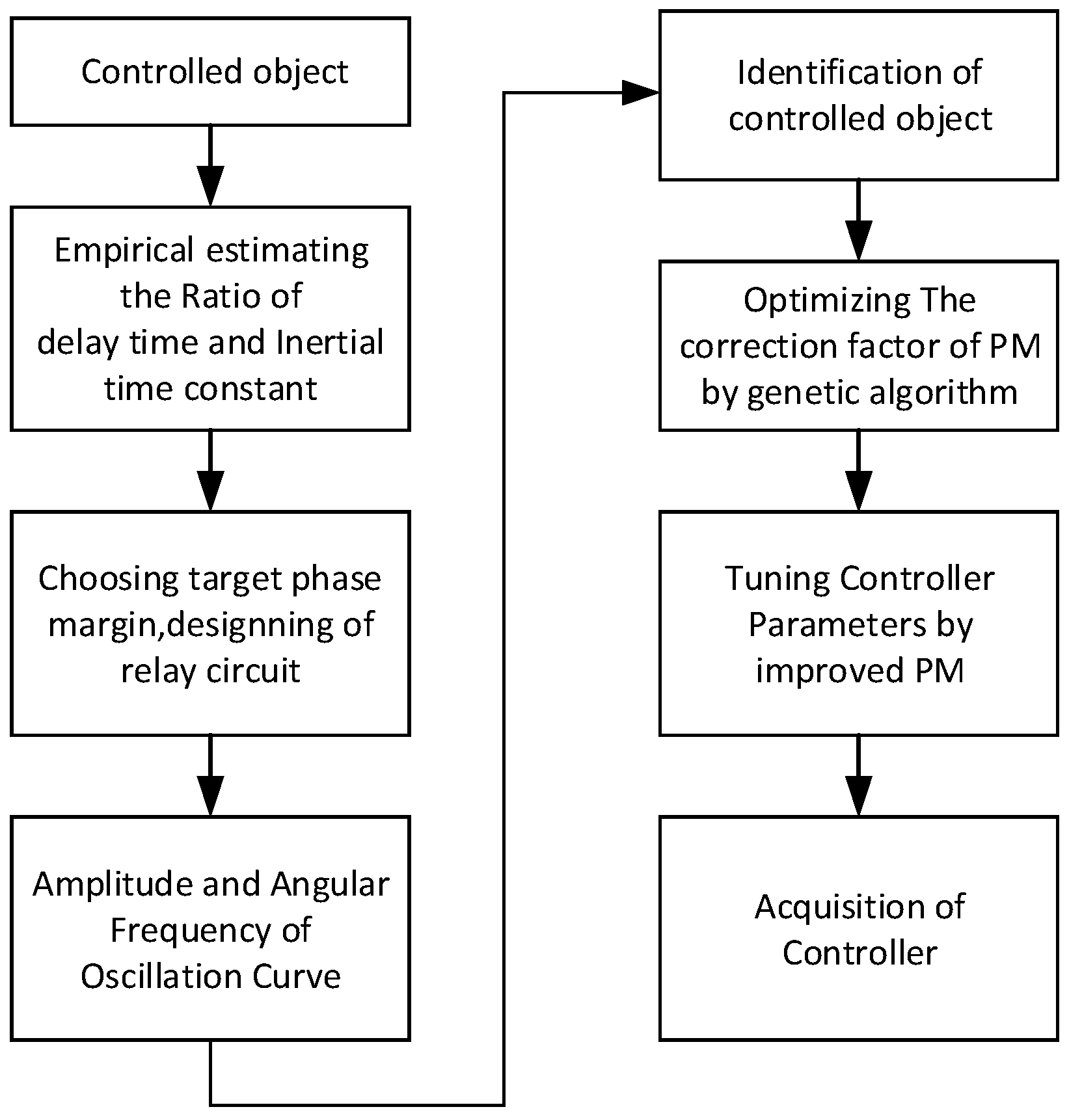
In the basic relay characteristic tuning methods, when compared with the Z-N formula setting, the PM method has a higher stability and also overshoot and oscillation times of the control curve are lower. Compared with the SPAM method, the PM method does not need to set a target amplitude margin and has no requirement for the amplitude margin of the controlled plant. However, the PM method cannot fix the thermal plant that does not meet the conditions of the relay characteristic method, such as the first-order inertia link. In addition, for the controlled plant with large delay characteristics, the control effect obtained by the PM method self-tuning is not satisfactory. Therefore, based on the traditional PM self-tuning method, this paper proposes an improved algorithm. It optimizes the selection range of the target phase angle margin by frequency characteristic analysis, then obtains a solution to estimate the target phase angle margin. The parameters of the oscillation curve output of the relay loop are used for model identification to obtain the transfer function of the control object. Then, the optimum algorithm is used to work out the correction coefficient of the PM method auto-tuning formula, and satisfactory controller parameters are obtained.

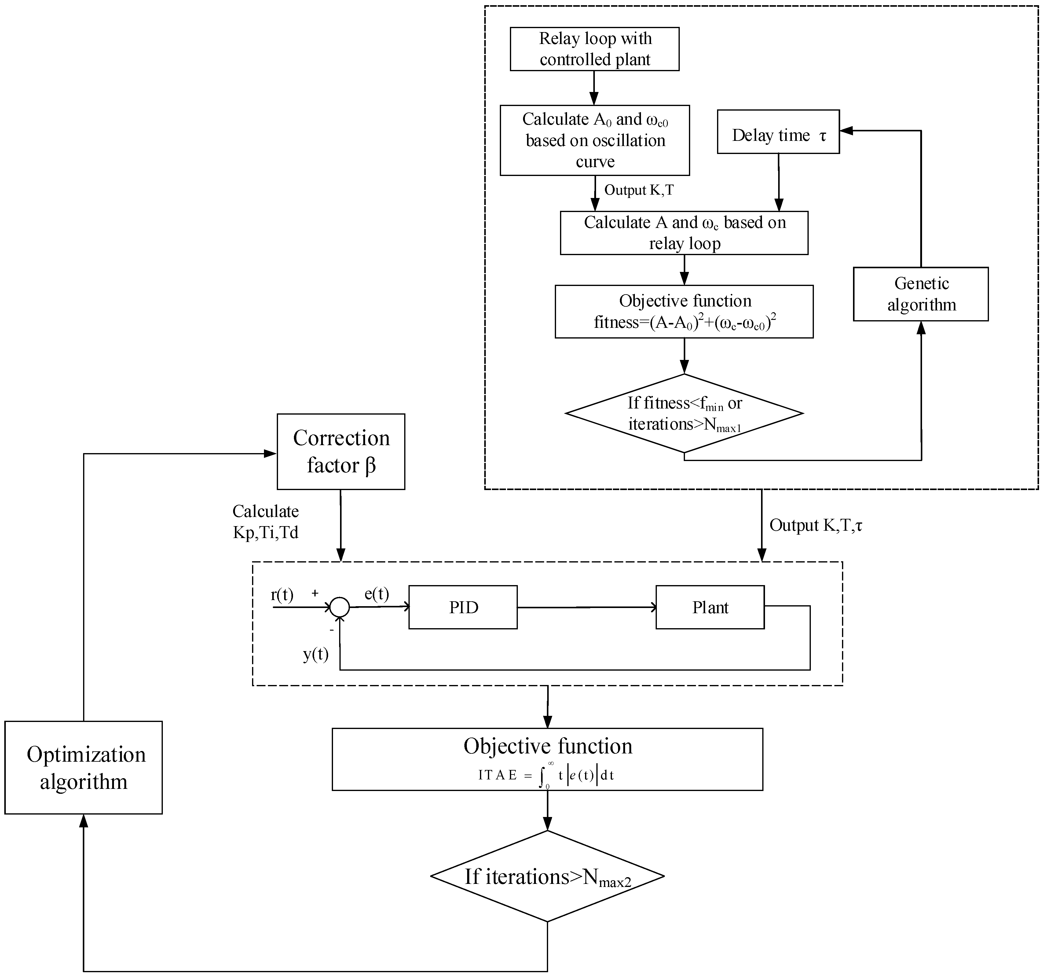
Hereinafter, Section 2 briefly introduces the basic principles of the traditional PM method and its shortcomings in the FOPDT plant. Section 3 analyzes the function of the target phase angle margin in the tuning process, and designs the correction factor from the tuning formula by the optimum algorithm. Section 4 simulates the superiority of the improved algorithm. Finally, the last section summarizes the characteristics of the improved PM self-tuning algorithm. The improved algorithm of the PID auto-tuning controller based on phase angle margin is shown in Figure 1.

2. Basic Principles and Disadvantages of the Traditional PM Method

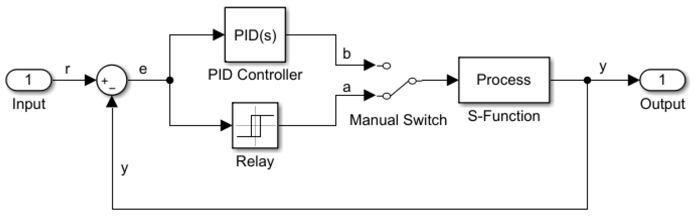
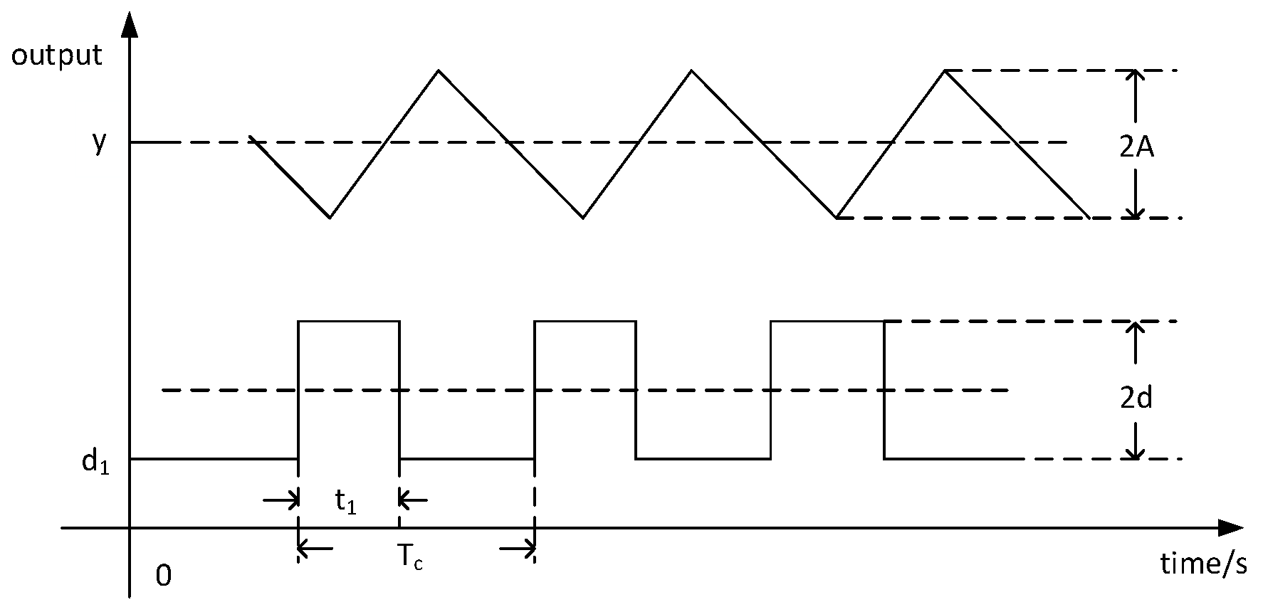
Figure 2 shows the auto-tuning principle of PID parameters based on the PM method. The process of calculating the controller auto-tuning parameters by the PM method is as follows: When the switch is thrown at terminal a, the hysteresis relay and the controlled plant form a unit negative feedback control loop. Select a set of relay thresholds and dead zones that can allow the system to output an oscillation curve under the action of the relay, and use the amplitude and period of the oscillation curve to estimate the coordinates of the critical point in the complex plane. There is a set of PID controller parameters that cause the critical point to move to the unit circle under the PID control and to meet the target phase angle margin. This set of controller parameters can be determined by the critical point coordinates and the target phase angle margin.

In Figure 2, r is the input, e is the deviation of the system and y is the output of the controller. The description function of the hysteresis relay is:

$$N(A)=\frac{4d}{\pi A}\sqrt{1-\frac{{\epsilon }^2}{A^2}}-j\frac{4d\epsilon }{\pi A^2}$$

(1)

where d is the output threshold value of the relay, d > 0. ε is the dead zone of relay, ε > 0. N(A) is the complex ratio of the first harmonic component and the input signal in the steady-state output of the relay under the action of sinusoidal signals. A is the amplitude of sine signal, A > ε.

Set the transfer function of the controlled plant as G(jω). When the switch is at terminal a, the closed-loop characteristic equation of the system is shown in Equation (2). The necessary condition for the limit oscillation of the system is that the equation below has a positive solution.

$$1+N(A)G(j\omega )=0$$

(2)

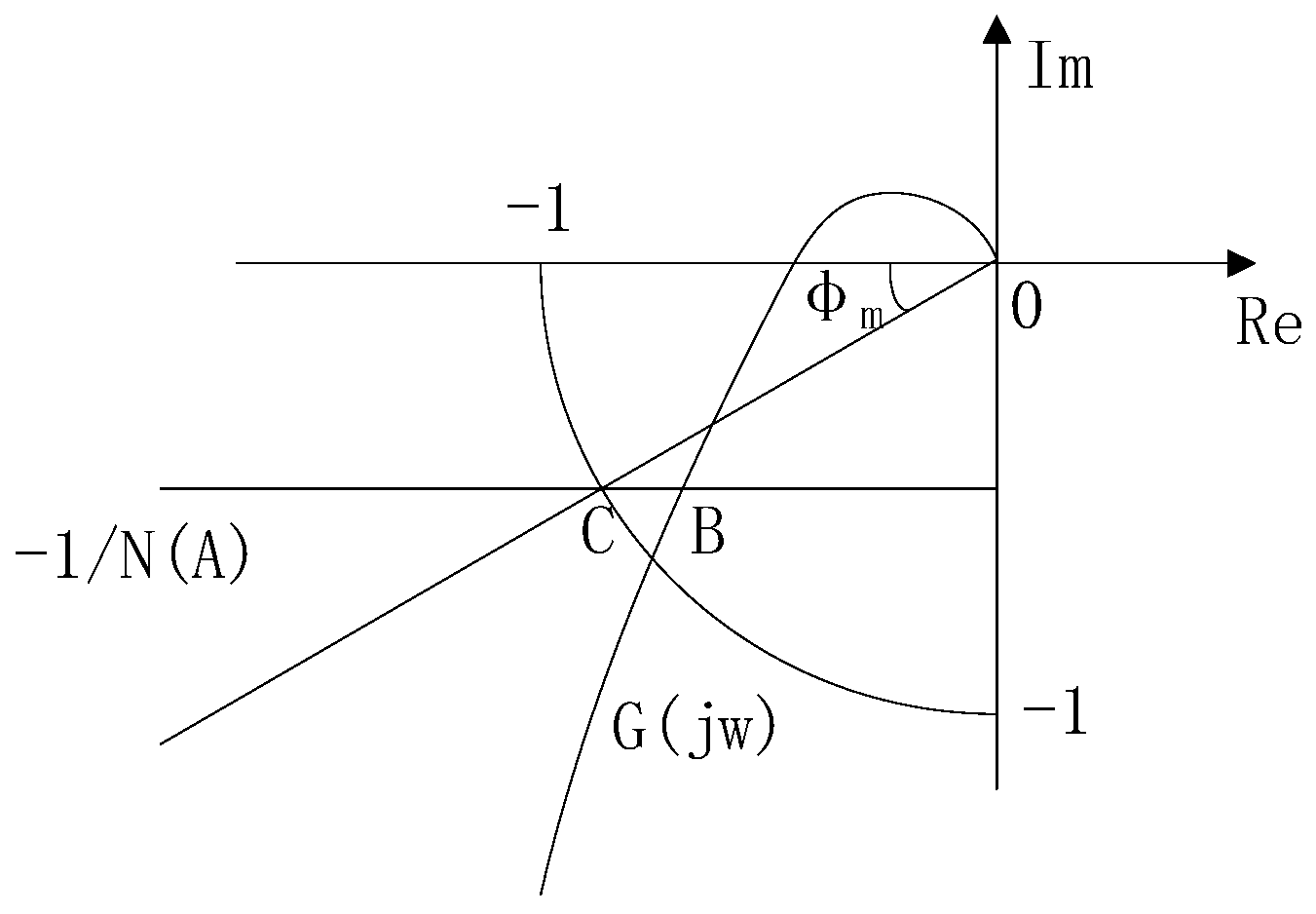
Figure 3 shows the Nyquist curve of the plant G(jω) on the complex plane and the negative reciprocal description function −1/N(A) curve of the hysteresis relay. The angular frequency where their intersection point B is located is the solution of Equation (2). Point B is the self-excited oscillation point of the closed-loop system, also known as the critical point. The negative reciprocal description function of the relay comes as Equation (3), then the coordinates of point B (−x, −jy) can be expressed by Equation (4).

$$-\frac{1}{N(A)}=-\frac{\pi }{4d}\sqrt{A^2-{\epsilon }^2}-j\frac{\pi \epsilon }{4d}$$

(3)

$$x=\frac{\pi }{4d}\sqrt{A^2-{\epsilon }^2},y=\frac{\pi \epsilon }{4d}$$

(4)

The form of the PID controller is shown in Equation (5). When the switch is thrown at terminal b (see Figure 2), the forward channel transfer function of the system is shown in Equation (6). The controller makes the Nyquist curve of the controlled plant move along these directions:$\overrightarrow{G(j\omega )}$, $\overrightarrow{G(j\omega )/j\omega }$ and $\overrightarrow{j\omega G(j\omega )}$, through proportional, derivative and integral actions, respectively. At a certain set of PID parameters, the critical point B can be moved to point C which meets the target phase angle margin requirement.

$$PID(s)=K_p(1+T_{d}s+\frac{1}{T_{i}s})$$

(5)

$$G_{forward}(s)=K_p(1+T_{d}s+\frac{1}{T_{i}s})G(s)$$

(6)

Assuming that the target phase angle margin is ${\phi }_m$, the coordinate of point C is $(-\cos {\phi }_m,-j\sin {\phi }_m)$, so:

$$\frac{\pi \epsilon }{4d}=\sin {\phi }_m$$

(7)

According to the coordinates of the B and C points in the complex plane and the vector relationship of the controller, the traditional PM method proposes the controller parameter tuning formula as follows:

$$\begin{array}{l}x=\frac{\pi }{4d}\sqrt{A^2-{\epsilon }^2}\\ T=\frac{(x-\cos {\phi }_m)\sin {\phi }_m}{{\sin }^2{\phi }_m+x\cos {\phi }_m}\\ K_p=\frac{{\sin }^2{\phi }_m+x\cos {\phi }_m}{x^2+{\sin }^2{\phi }_m}\beta \\ T_d=\frac{-T\pm \sqrt{T^2+\frac{\alpha }{4}}}{2{\omega }_c}\\ T_i=\alpha T_d\end{array}$$

(8)

where d is the output threshold of the relay, d > 0. ε is the dead zone of the relay, ε > 0. A is the amplitude of sine curve when the controlled plant oscillates, A > ε. T is an intermediate parameter. α is the empirical coefficient, which is between 2 and 4. β is the correction coefficient, and the traditional PM method takes the correction coefficient as 0.5.

In this paper, the PM method is applied to the auto-tuning of controlled plants in thermal power plants. It is found that because the controlled plants of thermal power plants generally have first-order inertia plus pure delay characteristics, the traditional PM method cannot guarantee good control effects. There are two main problems as follows.

• The characteristics of the limit cycle object have not been studied in depth. To determine whether an object has a limit oscillation, the transfer function of the object is needed to be known. The oscillation condition is that the Nyquist curve of the plant intersects the negative inverse description function curve of the hysteresis relay in the third quadrant on the complex plane, and the limit cycle at the intersection is stable. However, during the actual engineering application process, the characteristics of the controlled plants are not fixed, the specific parameters are unknown, and the accurate Nyquist curve cannot be obtained.
• The PM method cannot obtain a stable PID control system when the plant delay is large. The amplitude margin of a system is related to the open-loop amplitude-frequency characteristic at the phase-crossing frequency. For a system with a large delay plant, the open-loop amplitude-frequency characteristic is the Nyquist curve of the large delay plant without a controller, with this curve having poor attenuation. The method by only moving the critical point on the curve cannot change the amplitude-frequency characteristic of the frequency band near the phase angle crossing frequency. Reflected on the complex plane, the PM method cannot guarantee the system amplitude margin with the PID controller to meet the stability requirements. For the large delay plant, the PID control system obtained by the simple PM method will have a step response with oscillation and even divergence, and the control effect is not good.

3. Basic Principle of the Improved PM Method

In order to solve these two problems, an improved PM method is proposed in this paper. For plants with first-order inertia and pure delay, the main contents include selecting a target phase angle margin according to the estimated characteristics of the controlled plant to obtain an oscillation curve under the control of a relay loop. The mathematical model of the controlled plant is identified through the oscillation curve of the relay control loop. Then, an algorithm is used to optimize the coefficients in the auto-tuning formula to tune the controller parameters with the smallest integrated time absolute error (ITAE) index.

3.1. Selection of Target Phase Angle Margin

In Figure 3, the coordinate of point C is $(-\cos {\phi }_m,-j\sin {\phi }_m)$, indicating that the distance is $\sin ({\phi }_m)$ from the origin to the intersection point of the negative reciprocal description function curve −1/N(A) with the negative imaginary axis. The value of $\sin ({\phi }_m)$ is related to the Nyquist curve of the controlled plant. The frequency characteristic curve of the FOPDT plant is in the shape of a spiral attenuation toward the origin, as shown in Figure 4. The coordinate of the first intersection Q between the curve and the negative imaginary axis is (0, −Ksin(τω_q)), where ω_q is the angular frequency at point Q. Therefore, the target phase angel margin should satisfy.

$$\sin ({\phi }_m)<K\sin (\tau {\omega }_q)$$

(9)

Set the controlled plant as $G(s)=\frac{K}{Ts+1}{e}^{-\tau s}$, its frequency characteristic is $G(j\omega )=\frac{K}{jT\omega +1}{e}^{-j\tau \omega }$, in which the real part is:

$$\mathrm{Re}[G(j\omega )]=\frac{K}{T^2{\omega }^2+1}[\cos (\tau \omega )-T\omega \sin (\tau \omega )]$$

(10)

The frequency characteristic curve needs to be satisfied that the real part of G(jω) equals to 0, i.e., $\mathrm{Re}[G(j\omega )]=0$, at the intersection point with the imaginary axis, so is simplified by Equation (10) to:

$$\tan (\tau \omega )=\frac{1}{T\omega }$$

(11)

Equation (11) is a transcendental equation with no analytic solution and infinite positive real number solutions. As the frequency $\omega$ changes from zero to positive infinity, the frequency characteristic curve approaches the origin in a spiral shape and has infinite intersections with the negative imaginary axis. Each intersection point corresponds with a solution, wherein the first intersection point Q far from the origin point corresponds with the smallest solution ω_q. Draw curves $f(\omega )=\tan (\tau \omega )$ and $g(\omega )=1/T\omega$ in a plane rectangular coordinate system, as shown in Figure 5. The tangent curve is a periodic curve that is symmetric about the axis of symmetry $\omega =k\pi +\pi /2(k\in Z)$, so:

$$0<\tau {\omega }_q<\pi /2$$

(12)

Suppose τ/T = 1/M, M > 0, then there is T = τM, and Equation (11) is converted to:

$$\tan (\tau \omega )=\frac{1}{M\tau \omega }$$

(13)

Equivalent to:

$$\tan (\omega )=\frac{1}{M\omega }$$

(14)

Let the solution of Equation (11) be ${\omega }_0\in \mathrm{\Omega }$, then the solution ω₁ of Equation (13) will satisfy:

$${\omega }_1=\tau {\omega }_0,{\omega }_0\in \mathrm{\Omega }$$

(15)

So:

$$M{\omega }_1=M\tau {\omega }_0=T{\omega }_0$$

(16)

That is to say, in Equation (11), when τ/T is known, the product of the solution of the equation and the inertia time T is constant, in other words:

$$T{\omega }_0=c$$

(17)

where the constant c is uniquely determined by Equation (14).

The frequency ω_q of point Q satisfies Equation (11), so the absolute value of the imaginary axis coordinate of point Q is also constant, that is:

$$\left|\mathrm{Im}[G(j{\omega }_q)]\right|=K\sin (\tau {\omega }_q)=\frac{K}{\sqrt{1+T^2{{\omega }_q}^2}}$$

(18)

To sum up, when the ratio of the delay time and inertia time of the controlled plant G(s) is determined, the upper limit of the target phase angle margin of the system is:

$$\max (\sin ({\phi }_m))=\min (\frac{K}{\sqrt{1+T^2{{\omega }_q}^2}},1)$$

(19)

In this paper, 18 points are taken in the range of $\tau /T\in (0,1.5)$, and the tangent function and inverse proportional function curves shown in Figure 5 are drawn. The angular frequency at point Q is obtained, and a list of coordinates of the imaginary axis of point Q on the complex plane is obtained (see

Table 1. The imaginary axis coordinate of point Q under each ratio τ/T.

τ/T	0.01	0.1	0.2	0.3	0.4	0.5	0.6	0.7	0.8
Ksin(τωq)	0.0996 K	0.3061 K	0.4192 K	0.4985 K	0.5591 K	0.6079 K	0.6481 K	0.6821 K	0.7111 K
τ/T	0.9	1.0	1.1	1.2	1.3	1.4	1.5	1.6	1.7
Ksin(τωq)	0.7362 K	0.7581 K	0.7773 K	0.7943 K	0.8094 K	0.8229 K	0.835 K	0.846 K	0.8559 K

). The phase angle margin represents the stability performance of the closed-loop system. The larger the value of ${\phi }_m$, the more stable the step response curve of the system under PID control, the less oscillation, but the slower the adjustment speed. The smaller the value of ${\phi }_m$, the more the step response curve oscillates and the faster the adjustment. When ${\phi }_m$ is between 10% and 50% of the maximum value, both the rapidity and stability of the system can be considered. At the same time, the larger the inertia time constant of the controlled plant itself or the larger the delay time relative to the inertia time, the smaller the value ${\phi }_m$ can take in the above range.

3.2. Controller Parameter Optimization

3.2.1. Problems in the Traditional PM Method Tuning Formula

When the amplitude and frequency of the critical oscillation and the target phase angle margin of the controlled plant are determined, the traditional PM method can tune a group of PID controller parameters according to Equation (8). However, it has been proven by experiments that when the correction factor β in Equation (8) is equal to 0.5, it may not meet the control requirements. Therefore, a new auto-tuning strategy is proposed here to improve the control effect of the controller. According to Equation (5), if the K_p value decreases, the proportional action, integral action and derivative action of the controller are weakened, thus reducing the oscillation times and improving the stability of the system. Therefore, the selection of the correction coefficient can directly affect the control effect obtained by the PM method.

In this paper, 0.05, 0.5 and 2.75 for β are respectively applied to the tuning formula of the controlled plant $G_1(s)=\frac{5}{50s+1}{e}^{-s}$, and determined the PID controller parameters and the step response curve, as shown in Figure 6 by Equation (8). The overshoot of the control curve when β = 0.5 is about 21%, and the adjustment time is longer than that of the curve with β = 2.75. When β = 2.75, the control effect of the controller is optimal, the curve overshoot is the smallest and the adjustment time is the shortest. Take 0.5, 2.75 and 8.45 for β and apply them to the tuning formula of controlled plant $G_2(s)=\frac{1}{100s+1}{e}^{-s}$, respectively, and find the PID controller parameters and the step response curve according to Equation (8) also. The result is shown in Figure 7. With β = 0.5, the overshoot of the control curve is about 25%, and the adjustment time is the longest. With β = 8.45, the controller has the best control effect—the overshoot of the curve is the smallest and the adjustment time is the shortest. It can be seen that a single correction coefficient for different control systems cannot guarantee that the control effect of the auto-tuning controller is satisfactory. Those PID controllers below are shown in

Table 2. PID controllers by different correction factors of G₁(s) and G₂(s).

G1(s)	PID Controllers	G2(s)	PID Controllers
β = 0.05	$PID(s)=0.0642+\frac{1}{133.2331s}+0.1371s$	β = 0.5	$PID(s)=1.2782+\frac{1}{12.2314s}+27.4576s$
β = 0.5	$PID(s)=0.6416+\frac{1}{13.3233s}+0.1371s$	β = 2.75	$PID(s)=7.0299+\frac{1}{2.2239s}+27.4756s$
β = 2.75	$PID(s)=3.5286+\frac{1}{2.4224s}+7.5406s$	β = 8.45	$PID(s)=21.6008+\frac{1}{0.7238s}+84.4251s$

.

3.2.2. Optimization of the Correction Coefficient

According to the previous analysis, the PM method can be applied to first-order inertial plants with different characteristics by modifying the correction coefficient in the setting formula. Since the thermal engineering plant characteristics of the actual power plant are not fixed and often change, this paper proposes the idea of changing the correction coefficient according to the characteristics of the controlled plant to ensure the control effect meets the requirements of stability and rapidity. The specific idea is shown in Figure 8, and the optimization method is shown below.

In Figure 8, N_max1 equals 100, representing the maximum number of iterations of the genetic algorithm, and f_min equals 10^-4, showing the maximum acceptable deviation to meet model accuracy requirements. N_max2 means the maximum number of iterations of the optimization algorithm and equals 100 as well. The termination conditions of genetic algorithm running are that the fitness function has been less than f_min, or the number of iterations has been larger than N_max1. During the running of the optimization algorithm, the termination condition is that the number of iterations has been larger than N_max2, and the minimum ITAE index can be located during the iterative process.

After the target phase angle margin is selected, the ratio of the dead zone and the threshold value of the relay can be designed according to Equation (7), wherein the dead zone is larger than the amplitude of noise, so that the system output of the relay control loop presents a critical oscillation curve. Then, the fast Fourier algorithm is used to analyze the frequency spectrum of the system output data to obtain the amplitude A₀ and angular frequency ω_c0 of the oscillation curve. The method of identifying the controlled plant using the amplitude A₀ and the angular frequency ω_c0 is described below.

Assuming that the controlled plant is $G(s)=\frac{K}{Ts+1}{e}^{-\tau s}$, connect the actual controlled plant to the relay controlled loop, and the output of the system generates critical oscillation. The oscillation waveform and the output waveform of the relay are shown in Figure 9.

First, identify the gain K of the plant. The average output value y of the oscillation curve is obtained by multiplying the output of the relay and the gain of the plant [16], that is:

$$y=K[\frac{(d_1+2d)t_1}{T_c}+\frac{d_1(T_c-t_1)}{T_c}=K(d_1+2d\frac{t_1}{T_c})$$

(20)

So the gain of the controlled plant is:

$$K=\frac{y}{d_1+2d(t_1/T_c)}$$

(21)

The modulus of the frequency characteristic of the controlled plant is $|G(j\omega )|=\frac{K}{\sqrt{T^2{\omega }^2+1}}$. The angular frequency of the critical point B is ω_c. According to Equation (4):

$$\frac{\pi A}{4d}=\frac{K}{\sqrt{T^2{{\omega }_c}^2+1}}$$

(22)

So the inertia time constant of the plant is:

$$T=\sqrt{\frac{16d^2{K}^2-{\pi }^2{A}^2}{{\pi }^2{A}^2{\omega }_c^2}}$$

(23)

After calculating the gain K and inertia time constant T of the control object from Equation (21) and Equation (23), the delay time τ is optimized by a genetic algorithm. The specific process is as follows: It is known that each set of parameters K, T and τ can obtain a unique amplitude A and angular frequency ω_c of the critical oscillation curve through relay loop control and the selection of an appropriate target phase angle margin. Therefore, when K and T are determined, a unique τ can be found in a given range, so that the obtained A and ω_c are equal to the known amplitude A₀ and angular frequency ω_c0. A genetic algorithm is used here to find the variable τ that minimizes the objective function. The objective function is as follows:

$$fitness={({\omega }_c-{\omega }_{c0})}^2+{(A-A_0)}^2$$

(24)

Take the transfer function $G_3(s)=\frac{5}{50s+1}{e}^{-50s}$ as an example. Connect G₃(s) with the relay control loop to obtain the oscillation curve (see Figure 10). As can be seen from Figure 10, y = 1, d₁ = −0.8, d = 1, t₁ = 19 and T_c = 37, so the gain is K = 4.41. In Figure 10, the amplitude of the oscillation curve is A = 0.5125, and the angular frequency is ω_c = 0.1745, so the inertia time constant is T = 62.5221. Finally, the delay time τ = 56.8957 is obtained by a genetic algorithm. The identification results are shown in

Table 3. Comparison of identification results with actual values of the plant G₃(s).

Compared Values	K	T	τ
Actual value	5	50	50
Identification value	4.41	62.5221	56.8957
Deviation	11.8%	25.04%	13.79%

. Obviously, the error of the identification results is acceptable in engineering application.

After obtaining the mathematical model of the controlled plant, the correction coefficient is adjusted online by an optimization algorithm. The specific process is as follows: According to the amplitude, angular frequency and target phase margin of the oscillation curve output of the relay circuit, the PID controller parameters are calculated online by Equation (8), in which the correction coefficient β traverses a certain range, generally taking (0,10). The PID controller and the identified plant transfer function constitute a closed loop system. Give the set point of the closed-loop system a step signal, then the ITAE index can be calculated from the output curve. By optimization algorithm the minimum ITAE index can be located and also the optimal correction coefficient β, whose corresponding controller is the tuning result. Finally, the controller is used for the control of actual plants. The ITAE index is shown in Equation (25):

$$\mathrm{ITAE}={\displaystyle {\int }_0^{\infty }t\left|e(t)\right|}dt$$

(25)

4. Simulation Example

The main steam temperature is one of the most important controlled parameters in large boiler units of thermal power plants. Only when the main steam temperature is controlled within a reasonable and stable range can the efficient operation of the units be ensured. The commonly used main steam temperature control strategy is the cascade PID control. When adjusting the controller parameters of the outer loop, the inner loop system and outer loop controlled plant need to be fitted to a generalized plant first. According to [17], the generalized controlled plant function of the main steam temperature to the disturbance of the feed water of a 600 MW supercritical once-through boiler at 100% load is shown in Equation (25). An improved PM auto-tuning algorithm is applied to the model to obtain PID controller parameters.

$$G_4(s)=\frac{1.082}{70s+1}{e}^{-45s}$$

(26)

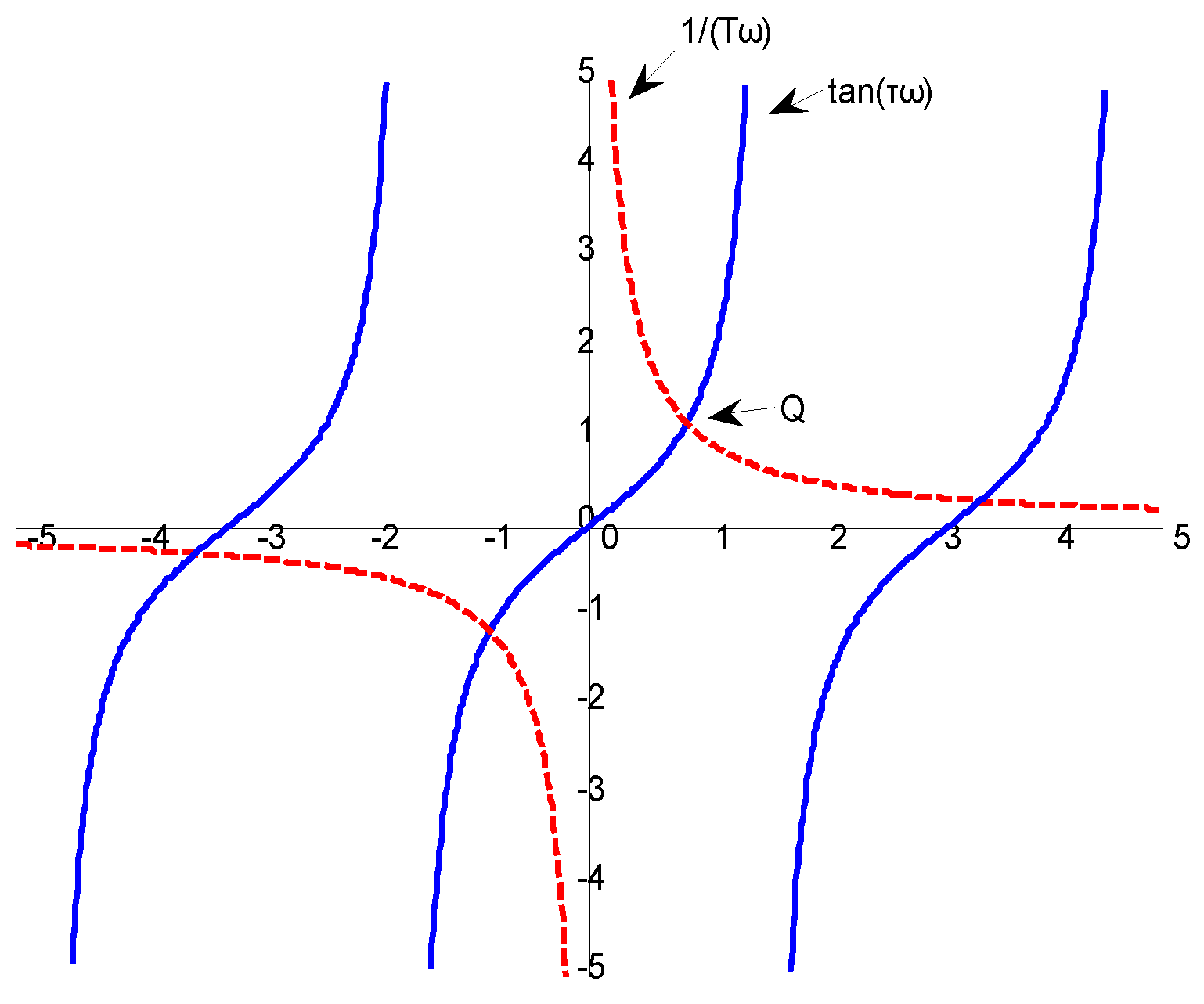
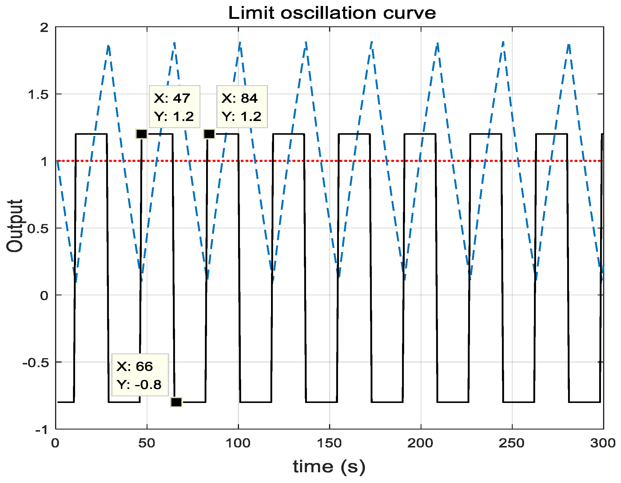
Here, the characteristics of the controlled plant have been determined, so the identification process is omitted. The ratio of the delay time of the plant to the inertia time constant is 0.6429. In the case of τ/T = 0.6 in Table 1, the sine of the target phase angle margin satisfies $\sin ({\phi }_m)<0.6481$, so $\sin ({\phi }_m)=0.4$ is available. According to Equation (7), the relay parameter should be designed as ε/d = 0.5357, where the relay threshold value is taken as d = 1. Connect the plant and the relay into a closed loop, and the oscillation curve can be obtained, as shown in Figure 11.

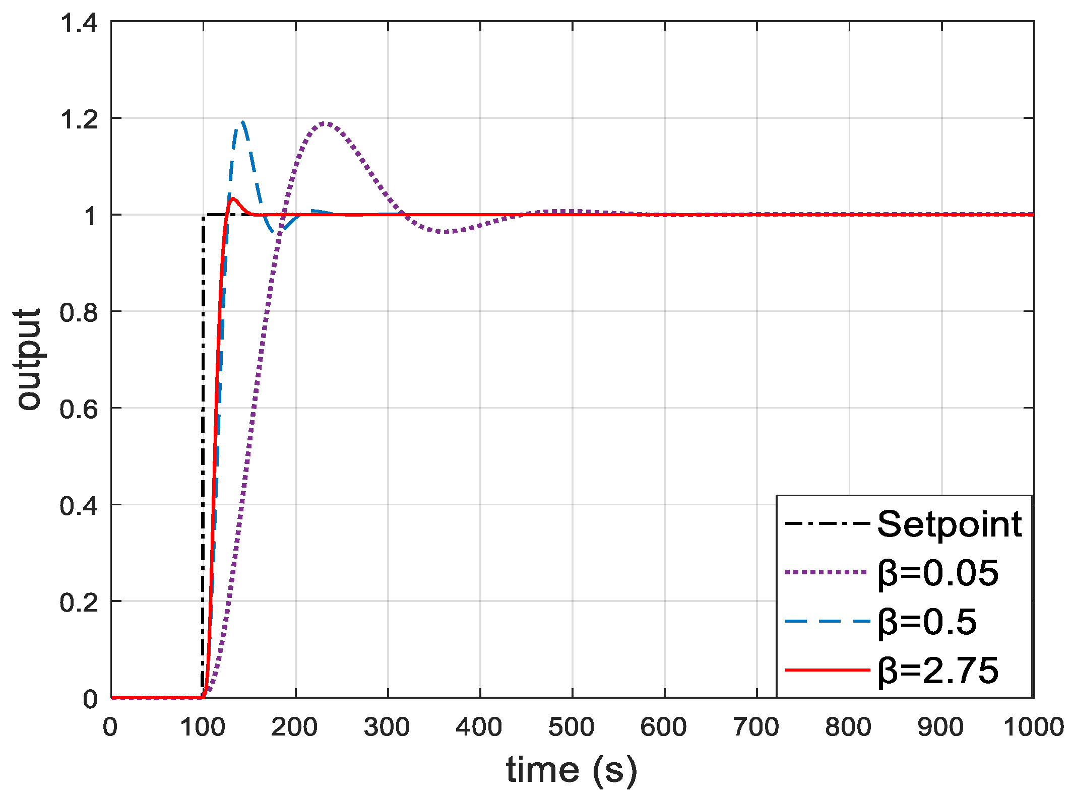
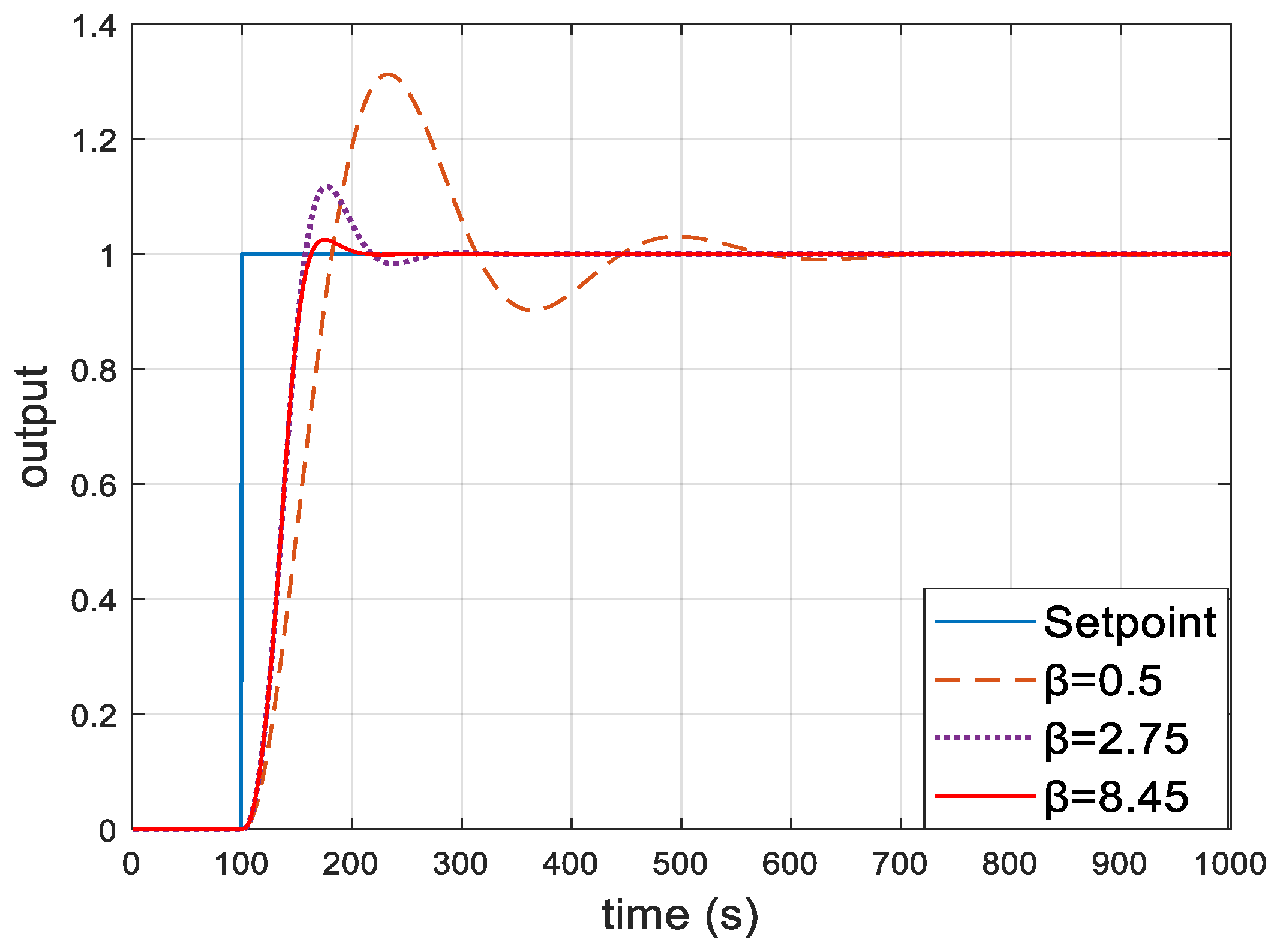
The controller parameters with the smallest ITAE index are calculated by an optimization algorithm for the correction coefficient within the range of (0,10), and algorithm results are shown in

Table 4. Results of relevant variables.

Parameters	A	ωc	x	β	T
Modified PM	0.4526	0.0403	0.2251	5.7	−0.7528

. The controller is:

$$PI{D}_{mPM}(s)=9.5435+\frac{1}{2.5964s}+59.1196s$$

(27)

The controller obtained through auto-tuning by the traditional PM method comes as:

$$PI{D}_{tPM}(s)=0.8371+\frac{1}{29.5994s}+5.1859s$$

(28)

In addition, the controller of the same plant is tuned by the Z-N method, and the obtained controller comes as:

$$PI{D}_{ZN}(s)=1.6879+\frac{1}{46.2224s}+32.9222s$$

(29)

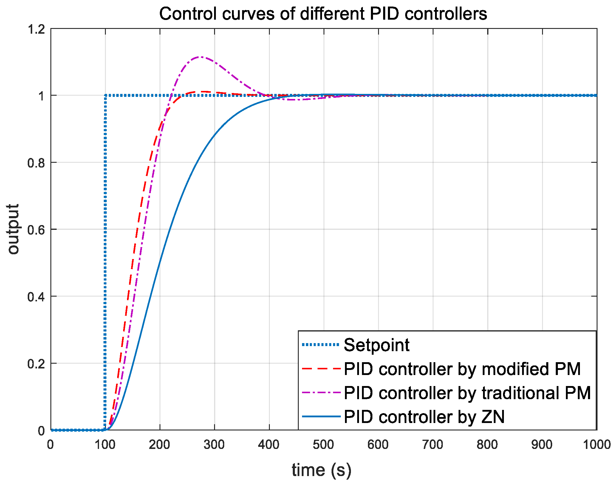
When the input of the set value of the plant is disturbed, the control effect of the controlled plant under the three PID controllers is shown in Figure 12, and the ITAE indexes of the three control performances is shown in

Table 5. Comparison of integrated time absolute error (ITAE) indexes by different PID controllers.

PID Tuning Method	ITAE
Modified PM	942.13
Traditional PM	12841
Ziegler-Nichols	6944.2

. The ITAE index of the improved PM method is much smaller than that of the Z-N method and the traditional PM method, and the control curve does not fluctuate frequently. The overshoot is only about 1%, and the adjustment time is about 100 s, which are both less than those of the other two control curves. In summary, the PID tuning improvement algorithm based on the phase angle margin obtains the best controller effect.

In order to more directly verify the results of the improved PM tuning algorithm applied in thermal power plants, this paper carried out a test on a 1000 MW ultra-supercritical unit. Under the steady-state condition of the 1000 MW unit, the PID controller of the secondary spray desuperheating system of the unit’s main steam temperature control is tuned. From the operating experience of the power plant, it can be seen that the secondary water spray desuperheating system is a large inertial element with delay, and the system characteristics will change according to the operating conditions. Therefore, it is difficult to manually adjust PID parameters.

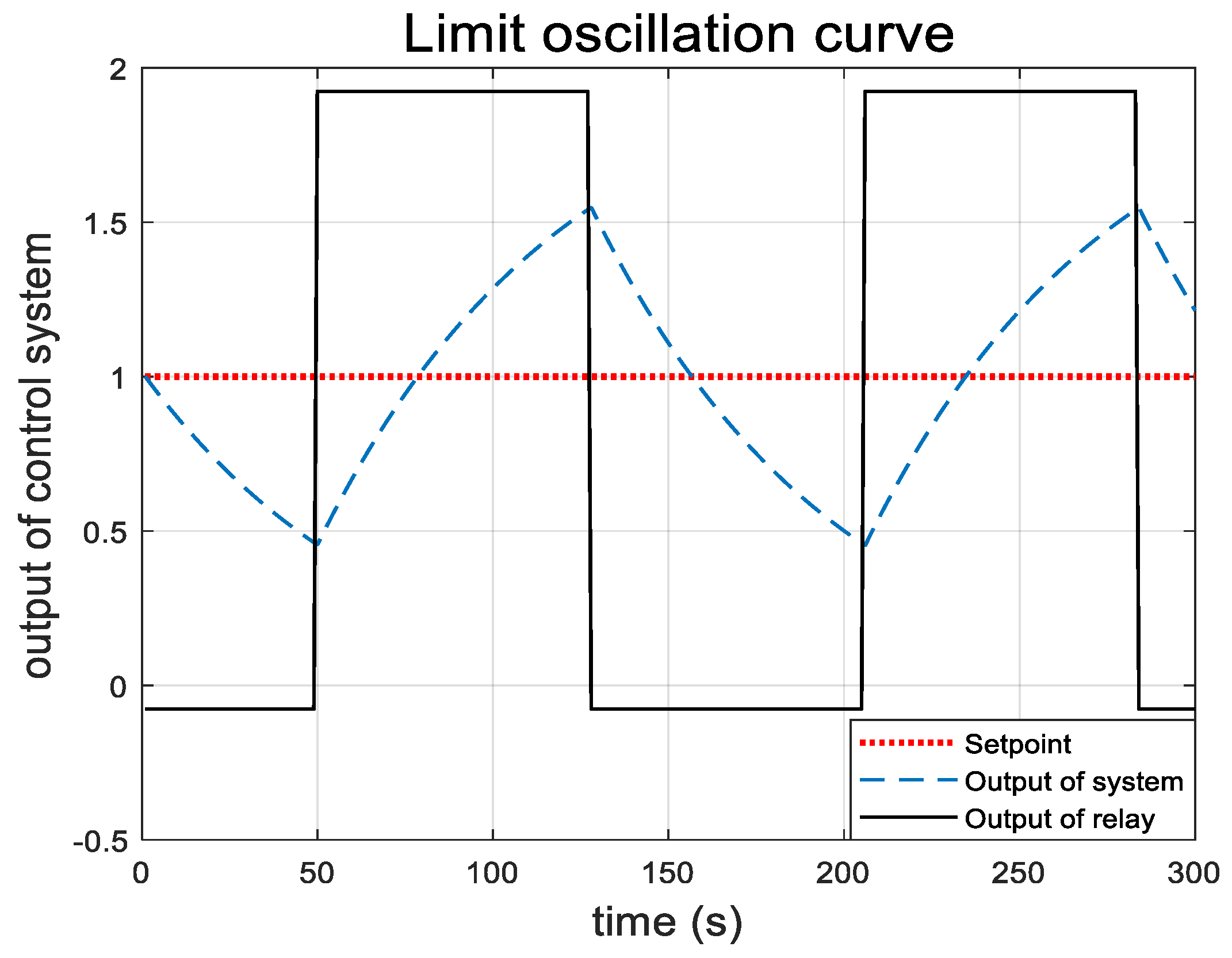
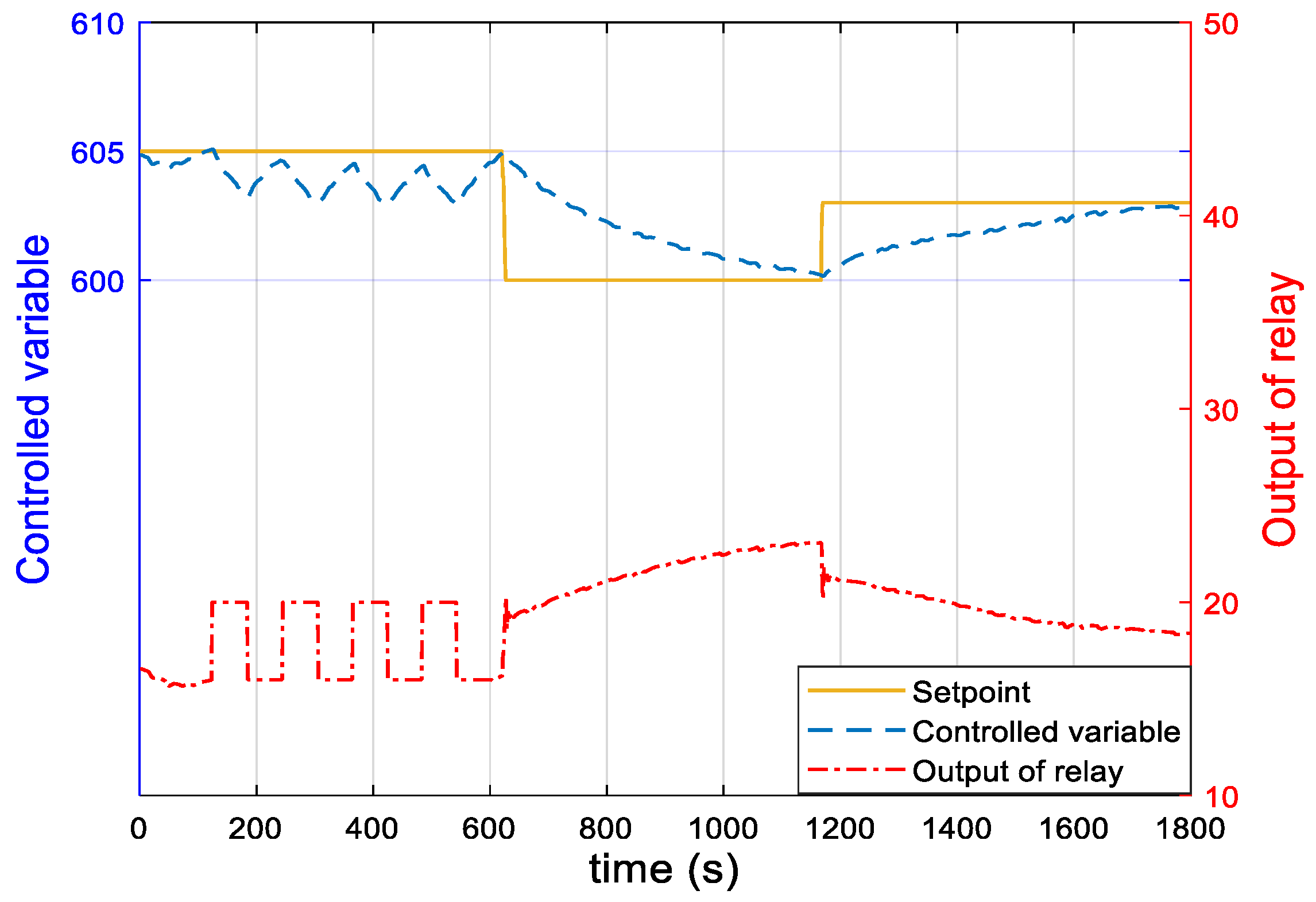
The experimental results with the main parameters during the tuning process are shown in Figure 13. The controlled system begins to enter the tuning mode at 100 s, and the controlled object forms a closed loop with the relay. The output curve of the relay is a square wave, and the system exhibits limit oscillation under the excitation of the square wave. The oscillation of the main steam temperature is shown by the blue dotted line, and the fluctuation of the main steam temperature is less than 2 °C. When it reaches 610 s, the tuning algorithm gives the PID control parameters, the controlled object switches from the relay loop to the PID control loop and the tuning mode ends. At 620 s, the system set point is reduced from 605 °C to 600 °C, and the main steam temperature gradually stabilizes to 600 °C under the PID control. Then, the set value is increased from 600 °C to 603 °C at 1170 s, and the main steam temperature is gradually increased to 603 °C. The experimental results show that the improved PM tuning algorithm can be applied to the control of thermal objects in thermal power plants. The tuning controller is calculated in Equation (30).

$$PID(s)=1.4198s+\frac{1}{38s}+19.15s$$

(30)

5. Conclusions

In this paper, the application of the PID controller auto-tuning parameter algorithm based on the phase angle margin is studied in the objected with first-order inertia and pure delay of a thermal power plant. The study found that the traditional PM method cannot always meet the control requirements for PID controller auto-tuning for different plants. In this paper, an improved tuning algorithm based on phase margin is proposed. By obtaining the maximum value of the target phase angle margin of critical oscillation by the frequency characteristics of the plant, it can ensure the critical oscillation of the controlled plant under the control of the relay, reduce the online auto-tuning time and ensure the safe operation of the controlled plant when oscillating. Furthermore, the amplitude and angular frequency of the limit oscillation waveform are obtained by combining the oscillation waveform. Based on this, the PID controller parameters are optimized online by combining the plant model identification. Also, the ITAE index as the optimization target is verified by simulation in the superheated steam temperature control system of the actual power station. The simulation results show that, compared with the traditional PM method and Ziegler–Nichols method, the improved PM online auto-tuning algorithm proposed in this paper can effectively improve the control quality of the plant, and the system adjustment is faster and the overshoot is smaller.

In addition, this paper tunes the parameters of the PID controller of the secondary sprinkler cooling system for the main steam temperature control of a 1000 MW ultra-supercritical unit under full load and steady state conditions. The experimental results show that the oscillation amplitude of the controlled variable is safe and reliable during the setting process, and the control effect is satisfactory. This improved tuning algorithm based on the phase margin provides a safe and feasible scheme for the application of a fast online self-tuning algorithm in power plants.

References

1. Jiang, S.; Zhang, X.; Huang, Z.; He, S. Improvement and research on PID controller of AGC. Henan Sci. 2018, 36, 186–192. [Google Scholar] [CrossRef]
2. Bai, Y. Design of PID controllers based on relayfeedback. Gansu Sci. Technol. 2016, 32, 10–12. [Google Scholar] [CrossRef]
3. Ziegler, J.G.; Nichols, N.B. Optimum settings for automatics controllers. Trans ASME 1942, 64, 759–768. [Google Scholar] [CrossRef]
4. Astrom, K.J.; Hagglund, T. Automatic Tuning of Simple Regulators with Specification on Phase and AmplitudeMargins. Automatica 1984, 5, 645–651. [Google Scholar] [CrossRef]
5. Hang, C.C.; Astrom, K.J.; Wang, Q.G. Relay feedback auto-tuning of process controllers—A tutorial review. J. Process Control 2002, 12. [Google Scholar] [CrossRef]
6. Liu, Y.; Sun, P. Application of auto-tuning of PID controllers based on relay feedback in the Buck-Boost circuit. Sci. Technol. Innov. 2016, 22, 12–13, 29. [Google Scholar] [CrossRef]
7. Yang, Z.; Liu, D. Design and implementation of self-tuning controllers based on PLC. Ind. Instrum. Autom. 2016, 3, 40–43, 98. [Google Scholar] [CrossRef]
8. Thuy, P.X.; Hiep, N.T. An Auto-Tuning Controller for Networked Control Systems. In Proceedings of the 2016 International Conference on Electronics, Information, and Communications (ICEIC), Da Nang, Vietnam, 27–30 January 2016. [Google Scholar] [CrossRef]
9. Gu, D.; Wang, J.; Zhang, Q. Auto-tune system using relay feedback test and model-based cascade control design. J. Northeast Norm. Univ. Nat. Sci. Ed. 2018. [Google Scholar]
10. Chen, F.; Yang, Z. PM algorithm of PID controllers self-tuning and its formula derivation. Acta Autom. Sin. 1993, 19, 736–739. [Google Scholar] [CrossRef]
11. Chai, T.; Zhang, G. The new auto-tuning algorithm of PID parameters based on phase margin and magnitude margin. Acta Autom. Sin. 1997, 23, 167–172. [Google Scholar]
12. Wang, L.; Xiao, K.; de Lillo, L.; Empringh-am, L.; Wheeler, P. PI controller relay auto-tuning using delay and phase margin in PMSM drives. Chin. J. Aeronaut. 2014, 27, 1527–1537. [Google Scholar] [CrossRef] [Green Version]
13. Ye, H. Application of improved BP neural network to self-tuning PID. J. Yunnan Minzu Univ. Nat. Sci. Ed. 2018. [Google Scholar]
14. Jiang, N.; Pan, W. Fuzzy self-tuning PID controller on fuel control in supercritical unit. Tech. Autom. Appl. 2018, 37, 32–35. [Google Scholar]
15. Wang, J.; Peng, Q.; Wu, H.; Xu, Y. Re-search on PID parameters self-tuning algorithms for dual motors in electric vehicle. Mech. Electr. Eng. Technol. 2018, 3, 37–38. [Google Scholar] [CrossRef]
16. Xie, Y.; Xia, S. Relay Self-tuning Method of PID Regulator Parameters. Control Decis. 1993, 77–79, 123. [Google Scholar] [CrossRef]
17. Wang, J. Internal Model Control for Main Steam Temperature Control System in Thermal Power Plant; North China Electric Power University: Beijing, China, 2014. [Google Scholar]
Figure 1. The diagrammatic sketch of the improved phase margin (PM) method.
Energies 12 01704 g001
Figure 2. Principle diagram of proportional-integral-derivative (PID) parameter auto-tuning based on PM method.
Energies 12 01704 g002
Figure 3. Nyquist curve of G(jω).
Energies 12 01704 g003
Figure 4. Nyquist curve of first order plus dead time (FOPDT) plant.
Energies 12 01704 g004
Figure 5. Tangent function and inverse proportional function curve.
Energies 12 01704 g005
Figure 6. Comparison of control effect by different correction factors of G1(s).
Energies 12 01704 g006
Figure 7. Comparison of control effect by different correction factors of G2(s).
Energies 12 01704 g007
Figure 8. Flow chart of algorithm for controller optimization.
Energies 12 01704 g008
Figure 9. Schematic diagram of oscillation curve and relay output waveform.
Energies 12 01704 g009
Figure 10. Limit oscillation curve of G3(s).
Energies 12 01704 g010
Figure 11. Limit oscillation curve of G4(s).
Energies 12 01704 g011
Figure 12. Control curves of different PID controllers.
Energies 12 01704 g012
Figure 13. Curves of setting process about main parameters.
Energies 12 01704 g013