1. Introduction
A thermosyphon is a type of natural convection loop. By proper arrangement of the heating zone and the cooling zone, the fluid in the loop changes in density, and the resulting thermal buoyancy drives the heat transfer of the working fluid. The cooling section and the heating section are usually placed on the upper and lower sides or on the left and right sides of the loop, respectively. Heating of the working fluid produces a lower density, which generates thermal buoyancy and upward flow, and the heat is radiated toward the cooling section. Gravity works against the working fluid as it flows upwards and assists it as it flows downward (i.e., in the same direction as the gravity). Because there is no need for an external driving force, a thermosyphon has considerable operational reliability. The self-adjusting mechanism and stability enable thermosyphons to be applied in an extensive range of applications, such as solar heating and cooling systems, coolers for reactors in nuclear power plants, geothermal energy systems, waste heat recovery systems, and electronic cooling systems. There are many considerations when designing a thermosyphon with good thermal efficiency, such as the choice of working fluid, the choice of wall material, the location of the heating and cooling sections, and the geometry of the loop [
1,
2,
3,
4,
5,
6,
7,
8,
9,
10].
Garrity et al. [
1] studied the instability of a two-phase thermosiphon with a microchannel evaporator and a condenser. Vijayan et al. [
2] analyzed the steady state and stability of single-phase, two-phase, and supercritical natural convection in a rectangular loop using a 1-D theoretical model. Misale et al. [
3] analyzed the influence of the thermal boundary conditions on the flow regimes inside the pipes and the stability of the thermosiphon. The results indicated that the larger the heating power is, the larger the flow rate; however, after becoming a two-phase flow, the flow rate is reduced due to the generation of bubbles. Lai et al. [
4] explored the influences of the aspect ratio, potential difference, heating power, and cooling temperature on the thermal performance of a rectangular natural circulation loop. Delgado et al. [
5] reviewed the information and application of two latent working fluids: phase change material (PCM) emulsions and microencapsulated PCM slurries.
Desrayaud et al. [
6] numerically investigated the instability of a rectangular natural circulation loop with horizontal heat exchanging sections for various Rayleigh number (Ra) values. The results show that vortices induce the occurrence of oscillations and the growth of temperature gradients. Buschmann [
7] analyzed the research on thermosyphons, heat pipes, and oscillating heat pipes operated with nanofluids based on 38 experimental studies and 4 modeling approaches. The results show that the effects related to the filling ratio, inclination angle, and operation temperature seem to be similar to those for classical working fluids. Huminic [
8] investigated the effects of volume concentrations of nanoparticles and the operating temperature on the heat transfer performance of a thermosyphon heat pipe with nanofluids using a three-dimensional simulation. The results show that the volume concentration of nanoparticles significantly reduced the temperature difference between the evaporator and the condenser. Sureshkumar et al. [
9] reviewed and summarized an improvement in the thermal efficiency and the thermal resistance of heat pipes with nanofluids. Gupta et al. [
10] presented an overview of the heat transfer mechanisms of heat pipes in terms of thermal performance.
Ho et al. [
11] obtained the relation of the Ra with the Reynolds number (Re) and Nusselt number (Nu) of a single-phase thermosyphon through experiments and numerical simulations. Vijayan et al. [
12] studied the effect of the heater and cooler orientations on a single-phase thermosyphon. Three oscillatory modes and instabilities were observed in the experiments. Misale et al. [
13] tested a thermosyphon with different tilting angles and found that the tilt angle affects the heat transfer effect, and the best effect was obtained with a tilt angle of 0° (vertical to the ground). Swapnalee and Vijayan [
14] obtained the relationship formula between the Re and Gr through experiments and simulations of single-phase flow in a thermosyphon and used the geometric parameter N
g to modify the Gr, crafting a prediction model that was applicable in four different heating and cooling modes. Thomas and Sobhan [
15] experimentally studied the stability and transient performance of a vertical heater–cooler natural circulation loop with metal oxide nanoparticles. Their results indicate that nanofluids containing aluminum oxide and copper oxide have superior heat transfer performances than pure water as the working fluid.
Because the literature on heating and cooling sections positioned in the two vertical sections of a rectangular thermosyphon is quite limited, despite the high potential of this application, this paper explores the natural convection heat transfer phenomenon of a rectangular thermosyphon with a geometric aspect ratio of 3.5. The boundary conditions of the loop heating section and the cooling section feature a fixed heat flux and a fixed wall temperature, respectively.
2. Materials and Methods
2.1. Scenarios and Test Cell Development
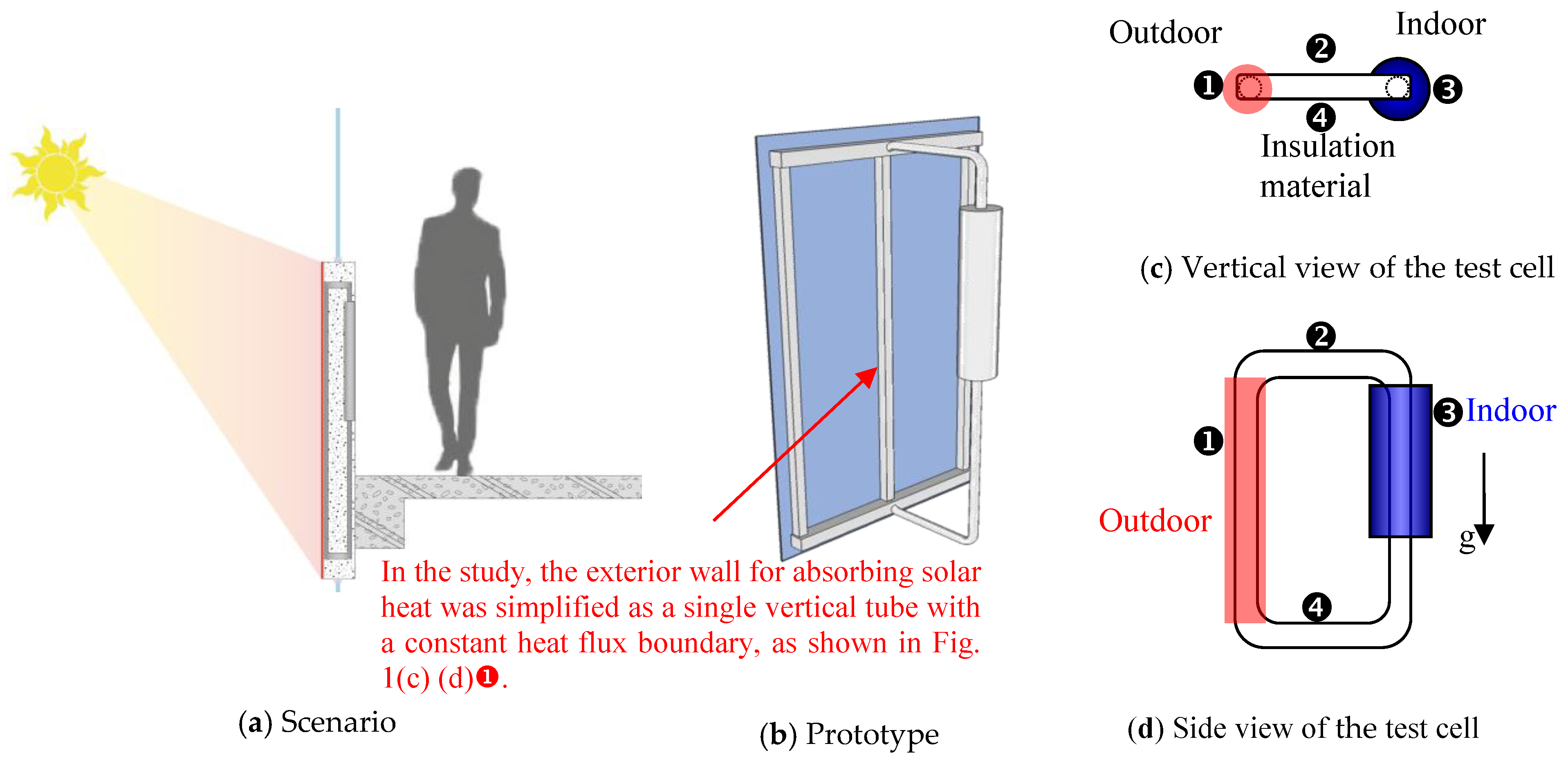
We aim to develop a structure that can harvest solar heat while attached to a metal wall (
Figure 1a). In addition to extracting heat energy, this building façade prototype can also effectively buffer the heat of the sun. Therefore, an energy-harvesting façade, as part of a solar thermal system and integrated with the building envelope structure, has been developed. To simplify the boundary conditions, we simplified the prototype into a rectangular natural circulation loop to further explore its basic heat flow mode and thermal performance.
The prototype design is shown in
Figure 1b. To simplify the boundary conditions and observe the basic heat flow performance, we simplified the prototype to the experimental test cell shown in
Figure 1c,d. The heat absorbing wall panel shown in
Figure 1b is first simplified to a boundary with a constant heat flux, as shown by ❶ in
Figure 1c,d. The vertical view in
Figure 1c shows the components without the insulation above the device for easy viewing. The side view in
Figure 1d shows the components without the heat insulation materials filling the space between the exterior wall and the interior wall to clearly illustrate the components of the circulation loop.
During the day, the working fluid in the circulation loop becomes a high-temperature fluid after absorbing heat from the outdoor heat source ❶. Driven by thermal buoyancy, the fluid forms natural convection, circulates along the horizontal circulation branch ❷ to the indoor heat sink, dissipates heat in the indoor heat sink ❸, and flows back to the outdoor heat source by another horizontal circulation branch ❹ via gravity; thus, a naturally flowing natural circulation loop is formed. The outdoor heat source ❶ is represented by a heated vertical tube; the indoor heat sink ❸ is a vertical section of an isothermal boundary.
2.2. Experimental Test Cell
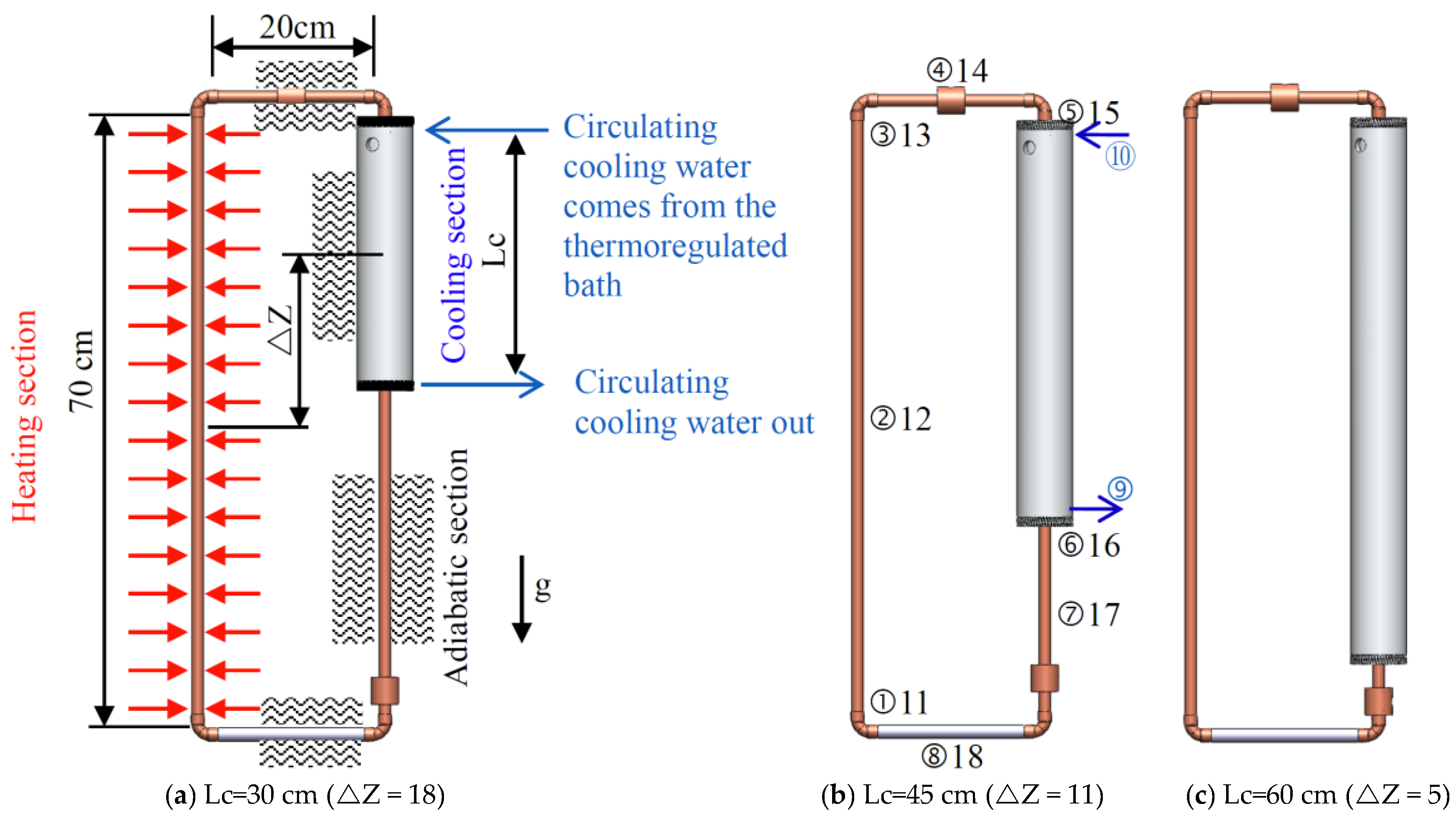
The experimental test cell can be divided into a rectangular loop comprising a heating section, a cooling section, and two adiabatic sections. The heating section and the cooling section are both located in the vertical portions of the loop (
Figure 2) and are described below.
2.2.1. The Rectangular Loop
The loop components in this test cell are all red brass tubes with high thermal conductivity, and the entire loop in the test cell has the same cross-sectional area, resulting in a constant tube flow value. The red brass tubes have an outer diameter of 12.7 mm and an inner diameter (
) of 11 mm. The length of the vertical heating section (Ly) is 700 mm, and the lengths (Lx) of the upper and lower adiabatic sections of the experimental test cell are both 200 mm; thus, the aspect ratio AR (=Ly/Lx) of the test cell is 3.5. To investigate the influence of the geometry of the experimental test cell on the heat transfer capability of the system, we set the cooling end length Lc to 30, 45, and 60 cm, as shown in
Figure 2a–c. The resulting potential differences (
are 18, 11, and 5, respectively.
2.2.2. Heating Section
The heating section is a boundary with a constant heat flux that simulates the practical application, and therefore, heating wire is used to generate heating at a fixed power. To increase the uniformity of the heating section, the electric wire is directly processed into the heating section, which is mainly composed of muscovite paper, electric heating wire and heat insulation materials. Because the tube material of the experimental test cell is conductive red brass, we must insulate the surface of the heating section tube before winding the heating wire around the heating section. Therefore, the soft muscovite paper, which is an excellent insulator and heat-resistant to 500–550 °C, is wound on the heating section for insulation purposes. The input electric power and the maximum voltage of the power supply are 60 W and 60 V, respectively, so the resistance is 60 Ω. Therefore, this experiment selects a heating wire with a resistance close to 60 Ω. The heating wire is 2.5 m in length, 0.25 mm in diameter, and 25.82 Ω/m in resistance per unit length.
2.2.3. Cooling Section
The cooling section is a simulated isothermal boundary condition. To test the effects of different height differences between the hot and cold ends, the water sleeve is set to lengths of 300, 450, and 600 mm. The cooling water sleeve is mainly composed of a water sleeve body and a water sleeve cover. The water sleeve body is a cylinder with an outer diameter of 61 mm and an inner diameter of 40 mm. Both ends of the water sleeve are water sleeve covers, and the center of each water sleeve cover has a hole that is approximately 11 mm in diameter. The thermosyphon passes through the holes in the cooling water sleeve, and the joints are fitted with O-ring grooves to prevent water leakage from the cooling water sleeve.
2.2.4. Insulation Materials
Except for the heating section and the cooling section, the remaining sections are adiabatic. To eliminate the effects of the external environment and heat loss during the experiment, 3-mm-thick insulating tape and a 40-mm-thick insulation pipe are wrapped around the body to effectively simulate adiabatic boundaries.
2.3. Experimental Apparatus
The device and data acquisition system includes a data acquisition unit (Yokogawa MX-100, Tokyo, Japan), PC, a flow meter (Fluidwell F110-P, Veghel, The Netherlands), a DC power supply unit (Gwinstek SPD-3606, New Taipei City, Taiwan), and a thermoregulated bath (RCB-412, New Taipei City, Taiwan).
2.3.1. Power Supply System
The heating wire of the heating section is connected directly to the power supply (Gwinstek SPD-3606); the output voltage and current are adjusted to provide an input power of 30–60 W, as required in the experiment.
2.3.2. Thermoregulated Bath
The isothermal boundary of the cooling section is established by circulating water from a thermoregulated water bath (RCB412) to establish the cooling section temperature Tc (30, 40, or 50 °C) required for the experiment.
2.3.3. Liquid Flow Meter
A flow meter (F110-P; Fluidwell) is used to monitor the amount of cooling water sent by the thermostatic water tanks in each test, with an average flow rate of approximately 35 mL/s.
2.3.4. Thermocouples
This study uses type-K thermocouples to measure the wall temperature and the fluid temperature along the loop. There are 17 thermocouple points embedded in each experimental test cell at the upper, middle, and lower positions of the heating section, at the inlet and outlet of the water sleeve in the cooling section, and along the adiabatic sections. The thermocouple points are shown in
Figure 2b. The thermocouple points numbered ①–⑧ measure the temperatures at the center point of the fluid in the tube; the thermocouple points numbered ⑨ and ⑩ measure the inlet and outlet water temperatures of the cooling sleeve; and the thermocouple points numbered 11–17 measure the temperatures of the outer tube wall.
2.4. Parameters
The relevant heat transfer parameters were calculated from the temperature measured by each thermocouple in the experimental test cell and the voltage and current supplied to the electric heating wire.
The input power can be obtained from the voltage V and the current I supplied by the power supply. Thus, the heat flux is /A. During the experiment, the heating from the power supply is not completely transferred to the fluid in the heating section. A small amount of heat enters the cooling section via axial heat conduction in the loop body or escapes into the environment, so the axial heat transfer must be deducted from the input thermal power first. Therefore, the corrected actual input thermal power is .
Modified Rayleigh number, Ra*
Parameters of the working fluid
- (1)
Flow rate of the working fluid ()
The temperature of the fluid in the rectangular loop increases in the heating section, causing the fluid to flow to the cooling section by convection. The flow rate of this flow varies depending on the amount of thermal power input to the heating section and the cooling conditions in the cooling section. In this experiment, the input heat power (
) and temperature difference (
) were used to determine the fluid flow rate in the tube.
- (2)
Nusselt number
- (1)
The average heat transfer coefficient of the cooling end is:
- (2)
The calculation of the Nu is as follows:
2.5. Experimental Uncertainty
The uncertainties in the measured quantities of this study were estimated to be ±0.1 °C for temperature, ±2% for the volumetric flow rate of the cooling water, and ±2% for the heat flux measured by the heat flow meters. Following the uncertainty propagation analysis [
16], the estimated uncertainties for the deduced experimental results were as follows: 5.1–26.2% for the heating flux, 3.1–25.8% for the cooling power, and 4.3–21.8% for the average Nu.
3. Results and Discussion
This experiment mainly discusses the effects of the heating power, cooling section temperature Tc, and height difference between the hot and cold ends ΔZ on the heat transfer phenomenon in a rectangular thermosyphon. The input thermal power is 30–60 W (the heating flux is in the range of 600–3800 W/m2); Tc is 30, 40, or 50 °C, and ΔZ is 5, 11, or 18 (Lc = 60, 45, or 30 cm, respectively).
Due to space limitations, only the experimental result of Tc = 40 °C is introduced; the heat flow phenomena for the other Tc values of 30 °C and 50 °C are similar to that of Tc = 40 °C and are not discussed further.
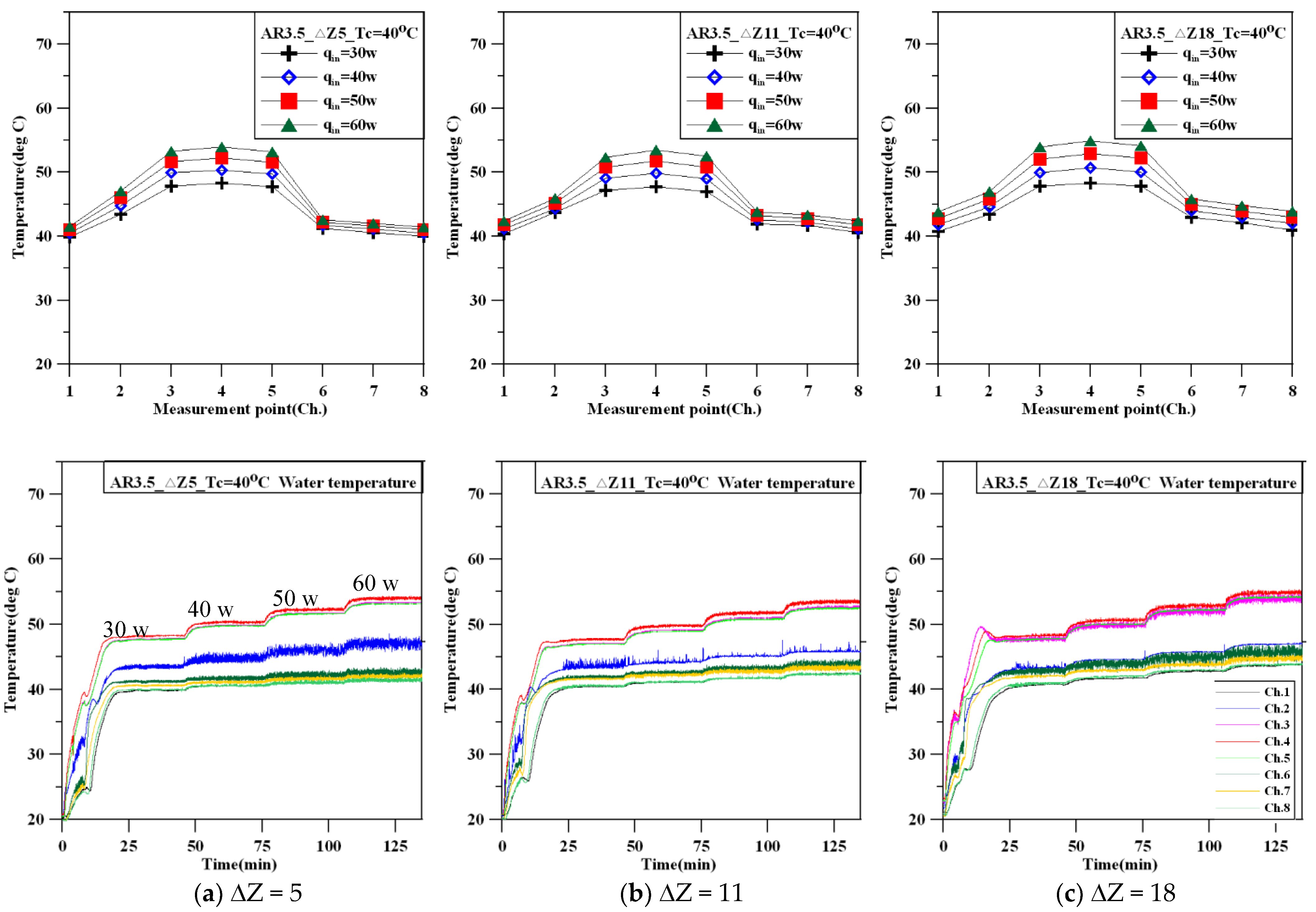
Figure 3 shows the change in working fluid (water) temperature in the loop at Tc = 40 °C as the thermal power increases. In the upper graphs, the x-axis represents thermocouple measurement points from Channel 1 to Channel 8, and the y-axis is the fluid temperature in the loop. In the lower graphs, the x-axis is experimental time.
Figure 3a shows the temperature variation of the working fluid (water) along the loop as a function of the heating power with a height difference ΔZ = 5 (Lc = 60 cm). First, the fluid in the thermosyphon is close to the stationary state. When the thermal power is set to 30 W, the temperature of the fluid in the heating section increases, and the fluid in the heating section slowly flows to the cooling section; it takes approximately 20 min to reach a steady state. Because the initial input of thermal power already initiated natural convection in the fluid in the thermosyphon, it only takes 5 min to reach a steady state after increasing the thermal power to 40 W, 50 W, and 60 W. When the thermal power is increased to 40 W, the temperature of the fluid in the middle section of the heating section (Channel 2) oscillates. The possible reason may be that the temperature boundary layer growth in the heating section is accompanied by a temperature mixing phenomenon formed by the fluid turning at the bend (near the heating section inlet). This oscillating phenomenon becomes more pronounced as the thermal power increases for a height difference ΔZ of 5.
Figure 3b shows the temperature variation of the working fluid along the loop as a function of the heating power with a height difference ΔZ of 11 (Lc = 45 cm). The temperature variation pattern of the fluid in the thermosyphon is similar to that of
Figure 3a, and it takes approximately 20 min to initially reach a steady state. After that, with further increases in the thermal power, the steady state is reached in approximately 5 min. The steady-state average temperature of the fluid in the thermosyphon shown in
Figure 3b is similar to that of
Figure 3a. Additionally, after the input thermal power exceeds 40 W, the temperature oscillation in the middle section (Channel 2) of the heating section begins to decrease. With increasing thermal power, the oscillation at Channel 2 becomes less noticeable.
Figure 3c shows the temperature variation with the height difference ΔZ of 18 (Lc = 30 cm). The temperature rise of the fluid in the thermosyphon is similar to the former two conditions, but the thermosyphon takes approximately 25 min to reach the initial steady state and approximately 5 min to reach new steady states when the heat power is increased.
Comparison of the three sets of data reveals that
Figure 3c, with a larger ΔZ, has a higher average temperature (approximately 2 °C higher) after the steady state is reached. The temperature difference between the highest and lowest power in
Figure 3c is slightly higher than in
Figure 3a. Comparison of
Figure 3a,b with
Figure 3c shows that when ΔZ is larger (the length of the cooling section is shorter), fluid temperature oscillations were observed at the exits of both the heating section and the cooling section (Channel 3 and Channel 6). This oscillating phenomenon is more pronounced as the thermal power increases. However, as ΔZ increases, the temperature oscillation magnitude in the middle section of the heating section (Channel 2) begins to decrease.
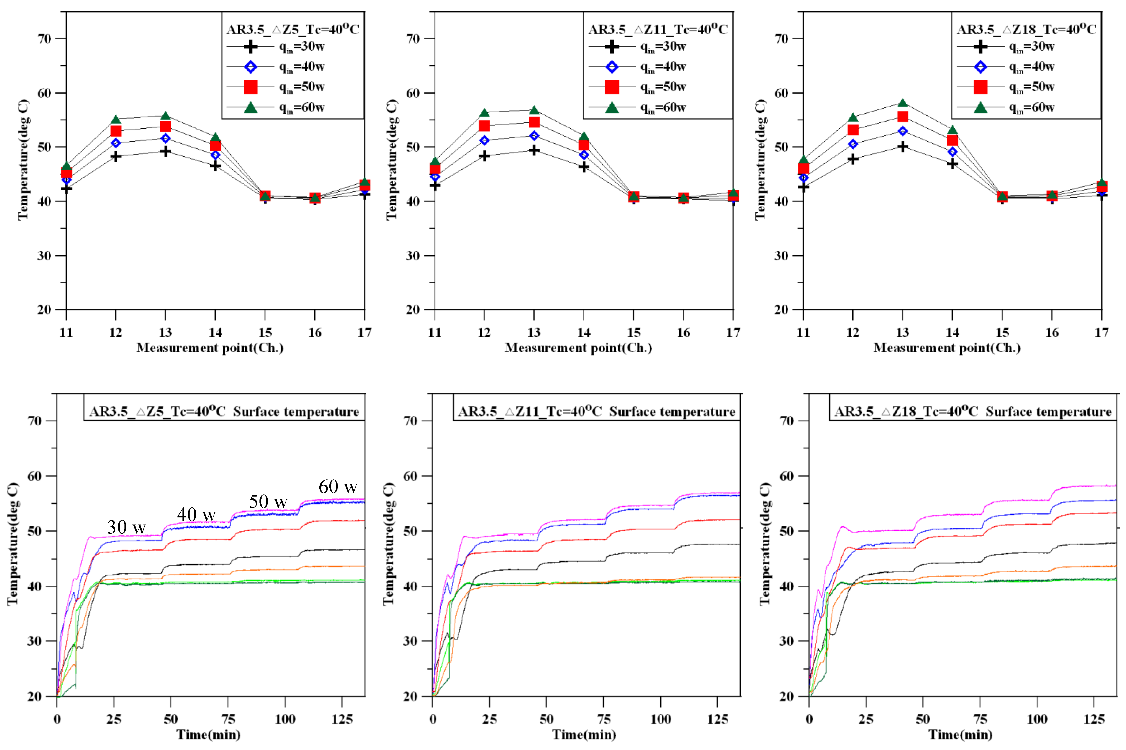
Figure 4 shows the change in temperature at each point in the outer wall of the thermosyphon as the thermal power increases. The temperature changes in each graph are quite similar. Due to the increase in heating power and the temperature rise of the fluid in the tube, the temperature of the outer tube wall at the end of the heating section is the highest. After entering the adiabatic section, the wall temperature of the outer tube wall decreases slightly. This phenomenon is mainly caused by the axial heat transfer of the tube wall. After entering the cooling section, the temperature of the outer tube wall begins to drop to Tc after cooling. However, after the cooling section, the temperature of the outer wall of the adiabatic section rises slightly due to the axial heat transfer. This temperature rise phenomenon is more obvious for ΔZ = 18 than for ΔZ = 5 and 11.
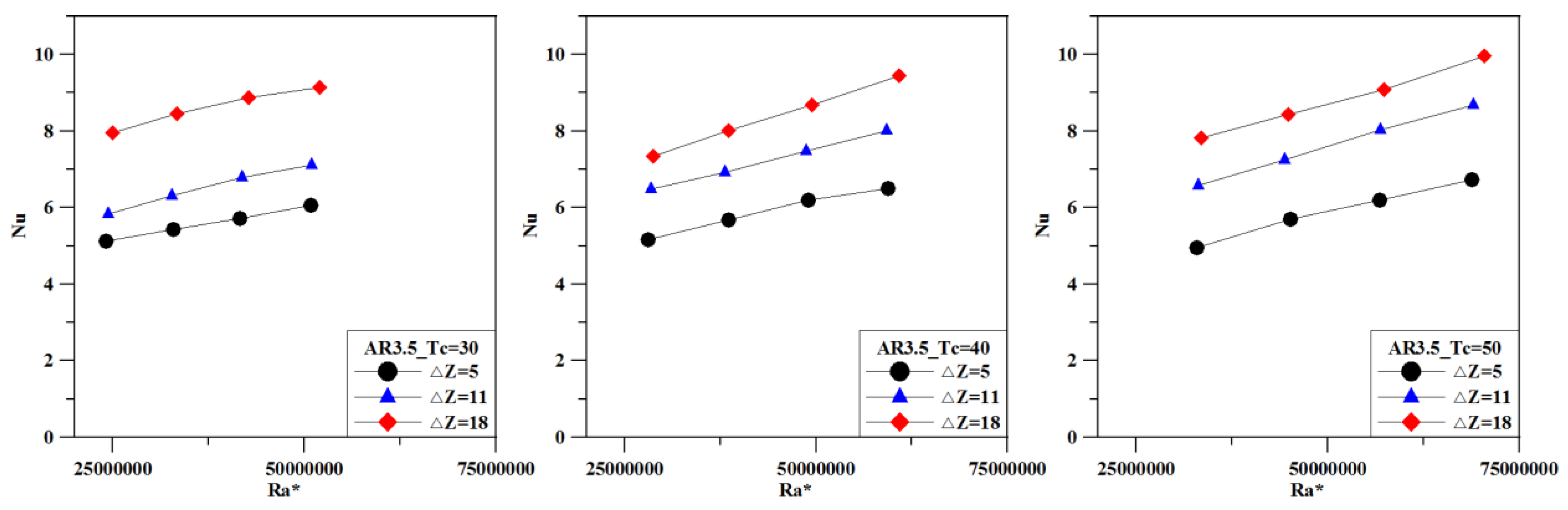
Figure 5 shows the relationship between the Nu and the modified Rayleigh number (Ra*) of the loop. Overall, the Nu is approximately 5–10. As Ra* increases, the natural convection intensity of the working fluid increases, so Nu increases. Under the designated geometrical configuration, the height difference between the cold and hot ends of the loop also affects the natural convection strength of the loop fluid. When the Ra* is fixed, as the height difference ΔZ increases, the Nu also increases. The effect of the cooling end temperature Tc on Nu is less significant. Therefore, if it is desired to increase the natural convection effect of the fluid in the tube, in addition to increasing the power of the heating section, the height difference between the hot and cold ends is also one of the controllable factors.
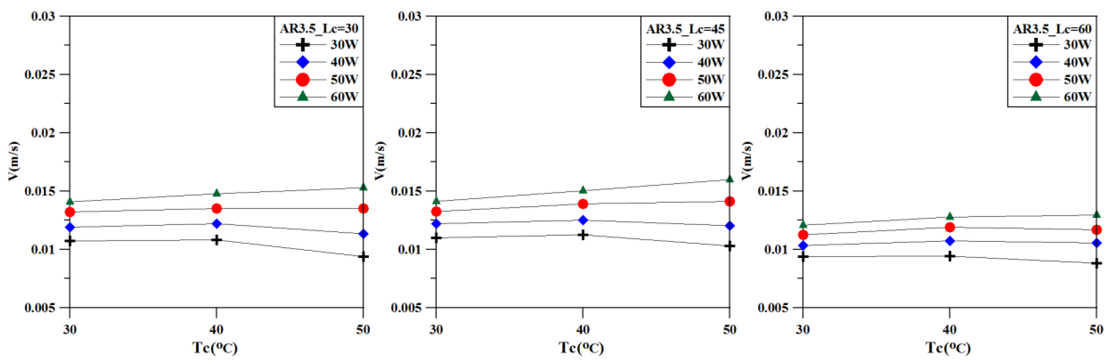
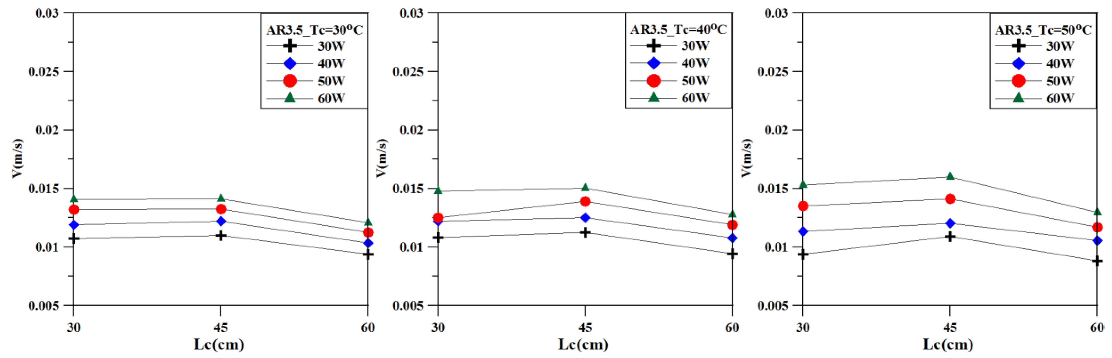
Figure 6 shows the relationship between the average flow velocity of the fluid and the cold end temperature. As the heating power increases, the average flow rate of the fluid increases significantly. With the increase in Tc, the average flow velocity of the fluid increases slightly in conjunction with a high heating power but decreases slightly in conjunction with a low heating power. The overall variation pattern indicates that the average flow velocity of the fluid is less affected by the cold end temperature than by the heating power. As the length of the cold end increases, the overall average flow rate decreases slightly (
Figure 7).
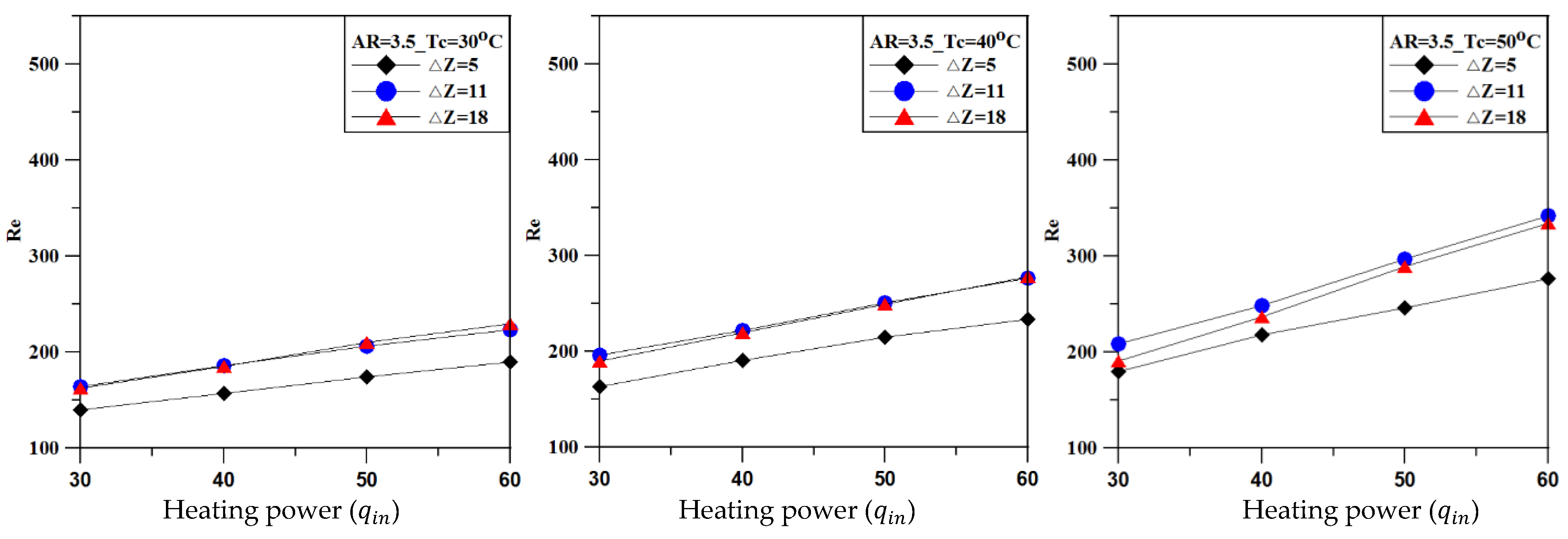
Figure 8 shows the Re and heating power (
) of the fluid in the tube. When the input heating power is 30 W, the Re values of the tube flow for different ΔZ and Tc values are approximately 150–200. With an increase in the heating power or Tc, the Re increases, but the influence of heating power on the Re is more significant than that of Tc. Furthermore, the Re of ΔZ = 11 is very close to that of ΔZ = 18. A higher heating power, Tc, or ΔZ can result in higher fluid flow intensity. For 60 W, Tc = 50 °C, and ΔZ = 18, the Re is approximately 345.


