Impact of Combined Demand-Response and Wind Power Plant Participation in Frequency Control for Multi-Area Power Systems


 ,
,  ,
,  and
and 
Abstract
:1. Introduction
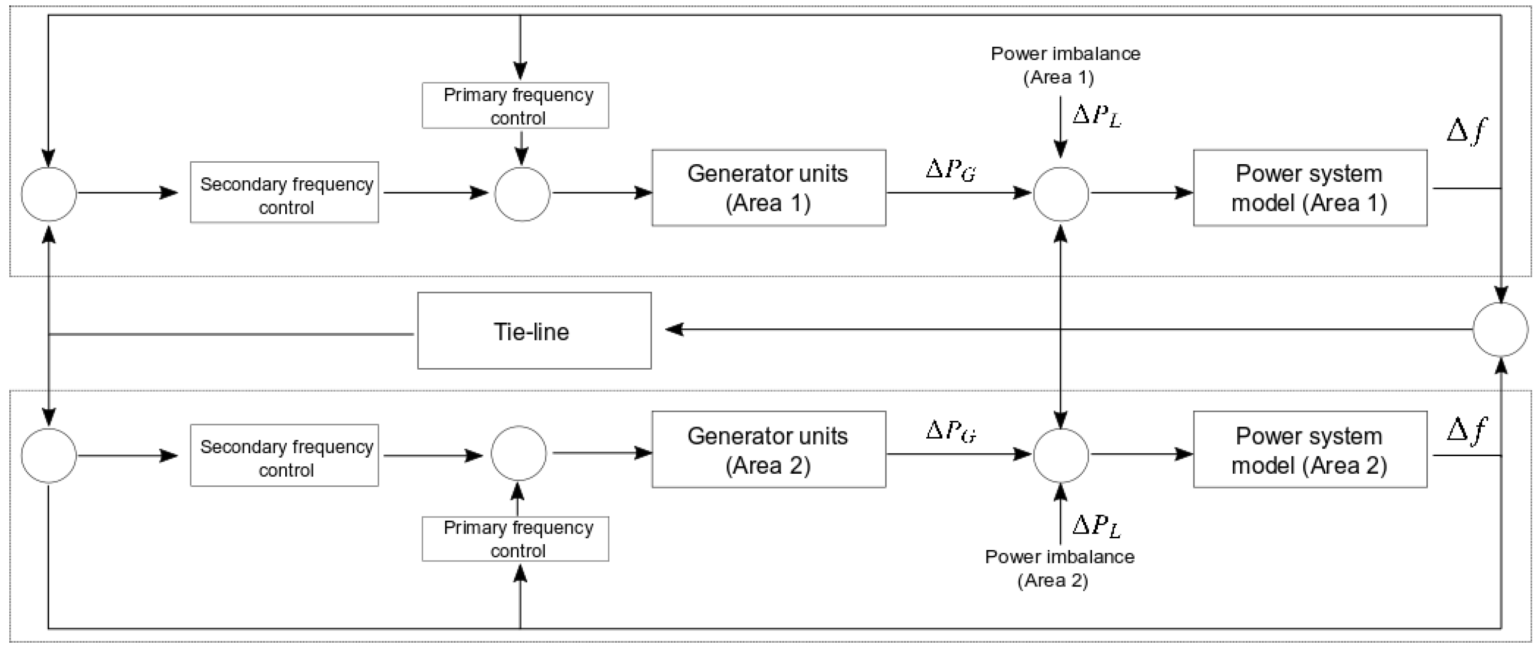
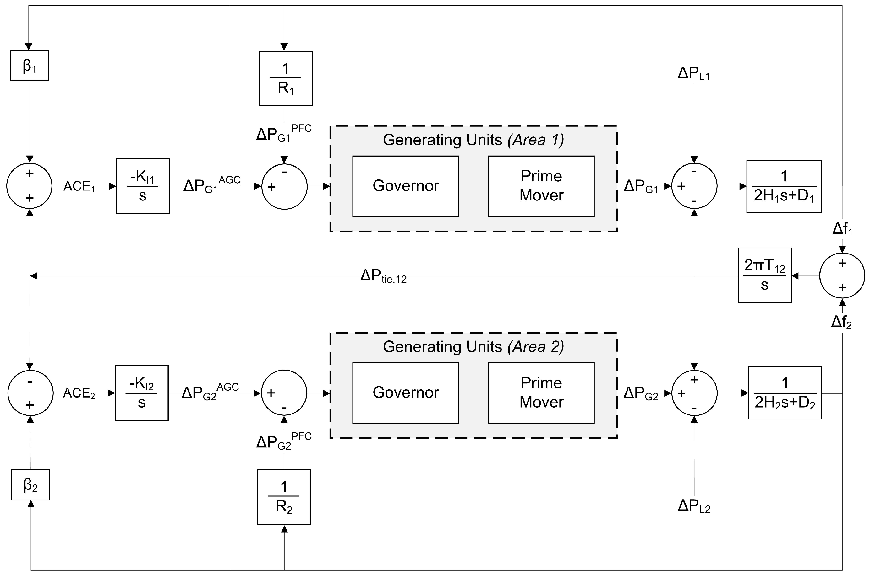
2. Power System Modeling: Wind Power Plant and Demand-Side Contribution to Frequency Control
2.1. Preliminaries
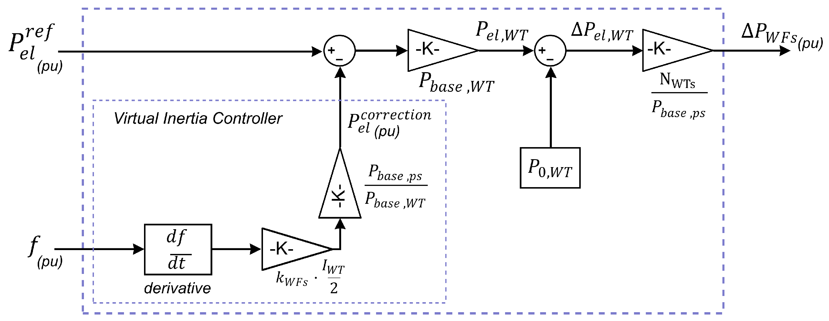
2.2. Wind Power Modeling
2.3. Demand-Side Modeling
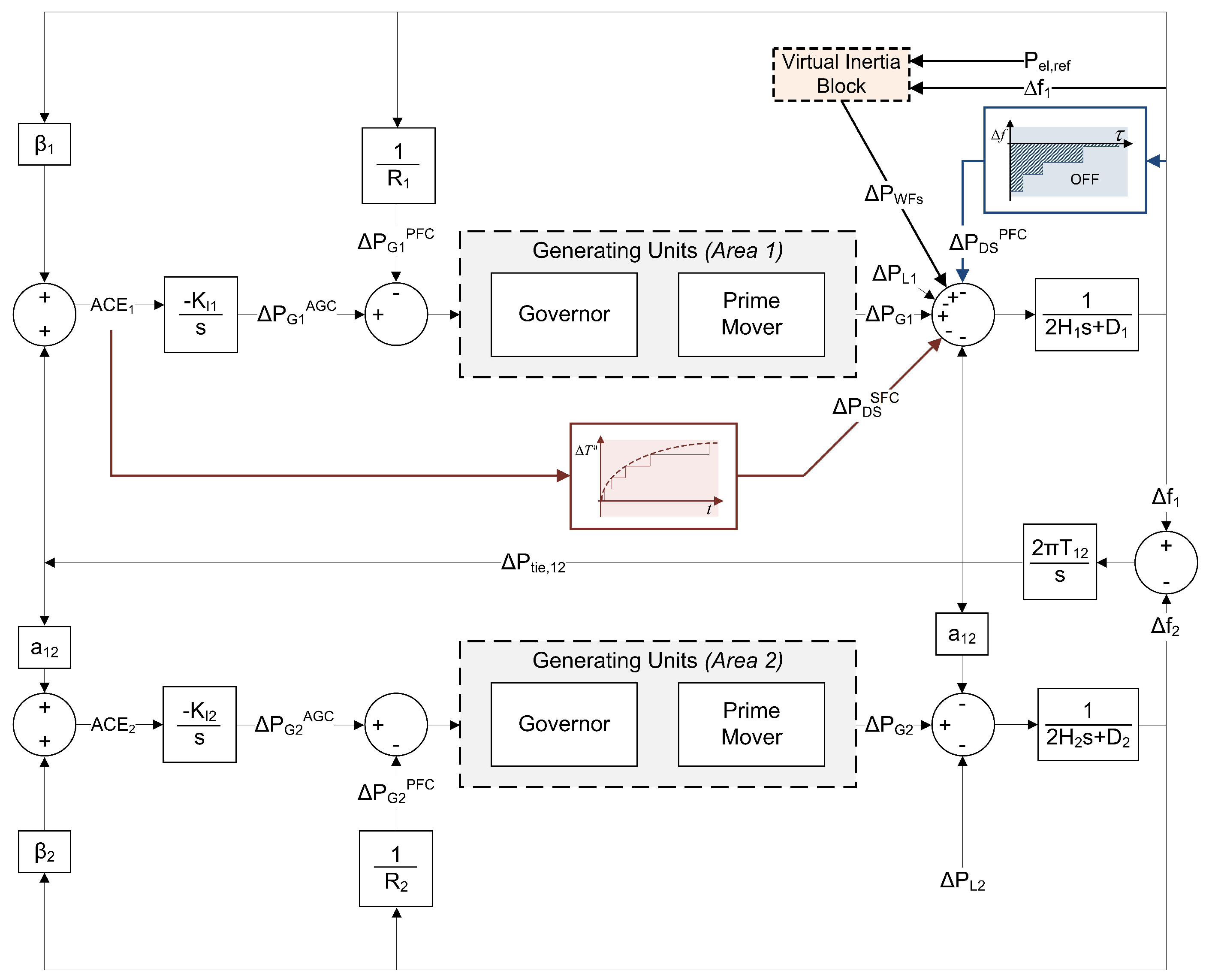
3. Demand-Side Contribution to SFC: Proposed Solution
3.1. General Description
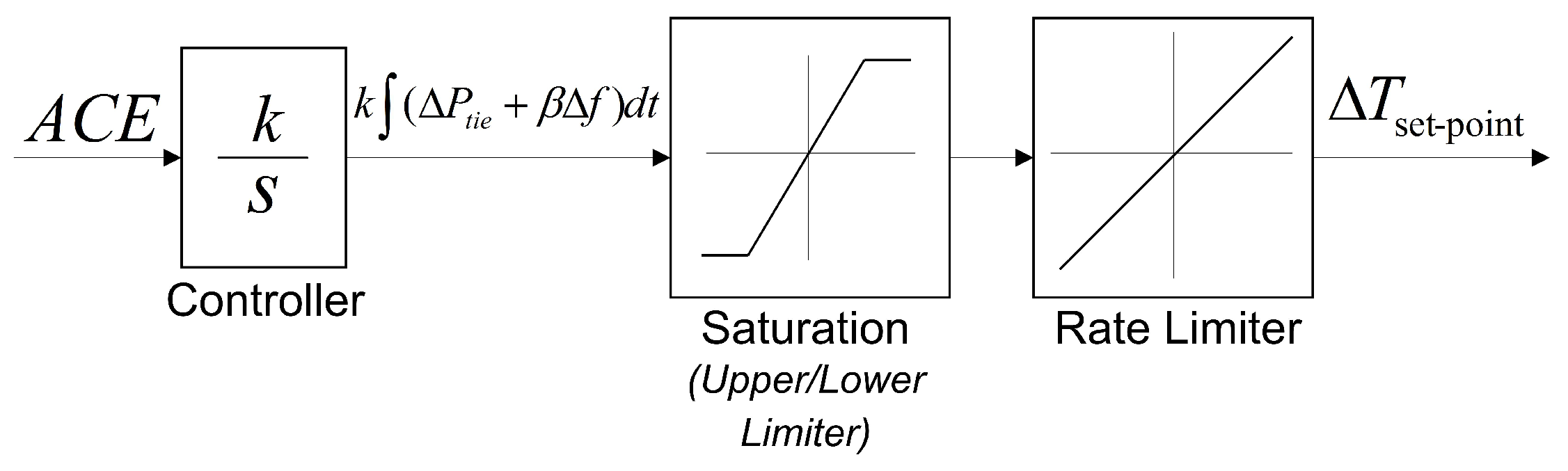
3.2. Implementation of Integral-Action Controller
4. Simulation and Results
4.1. Preliminaries
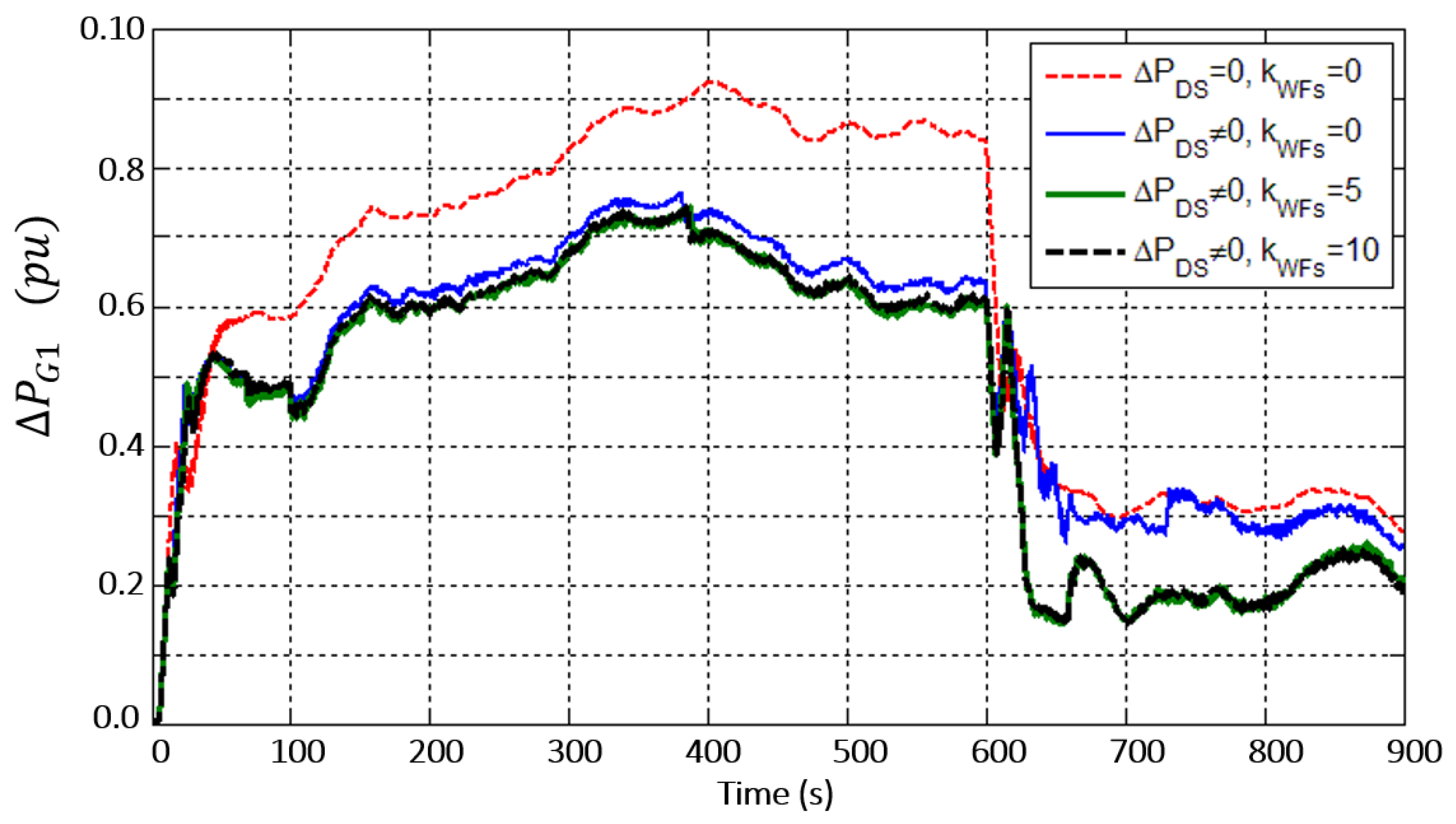
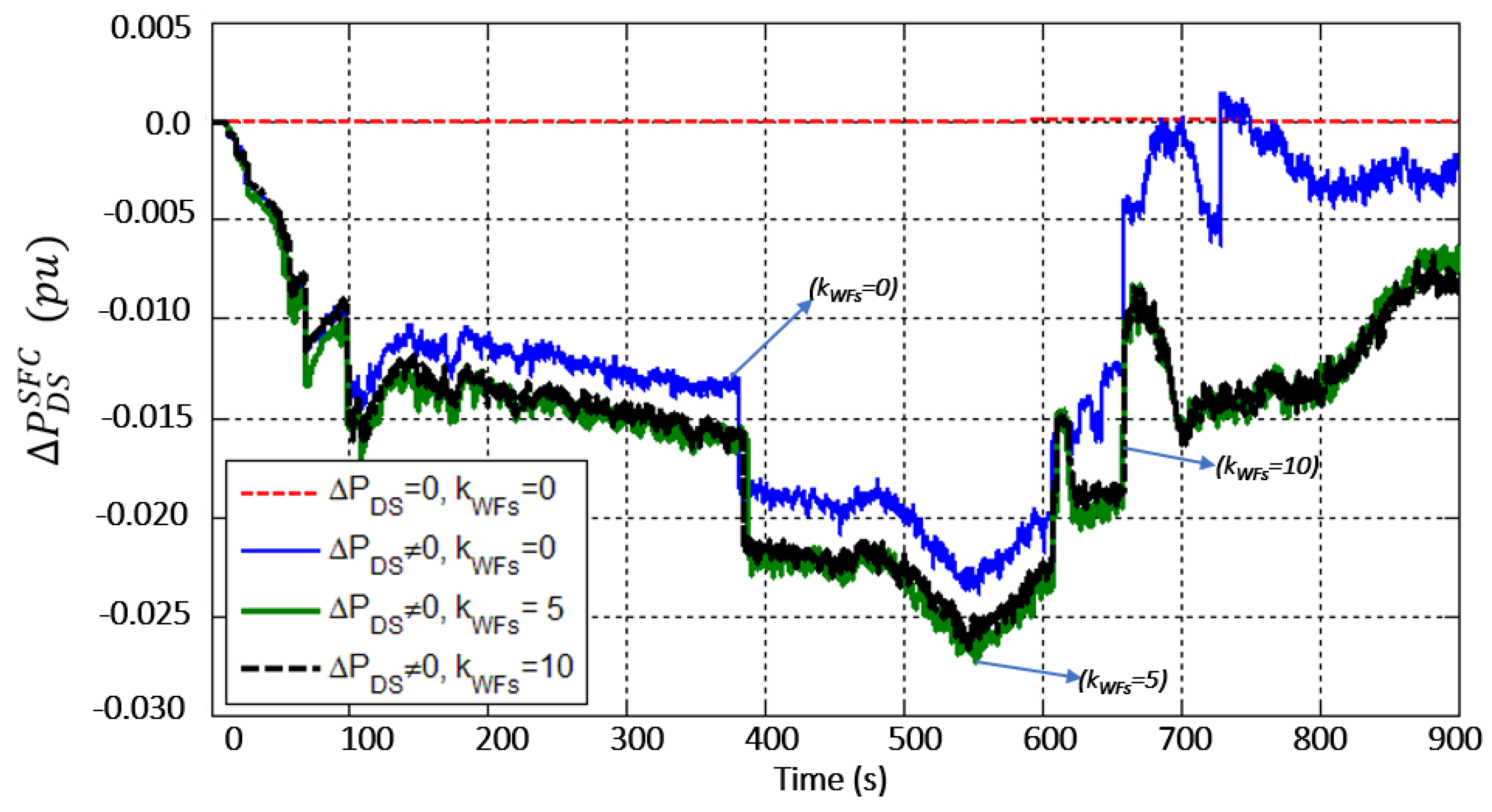
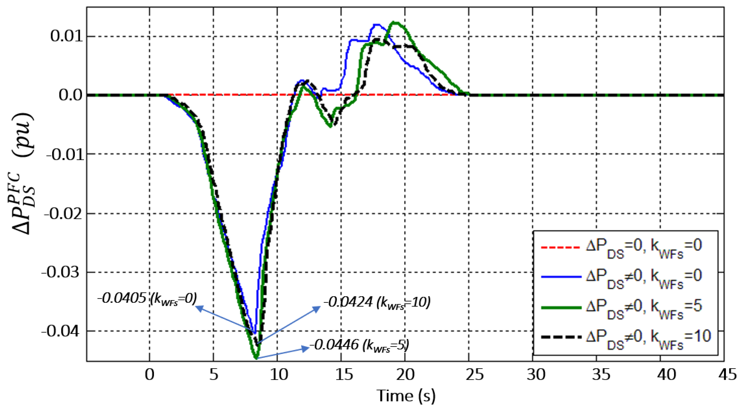
4.2. Results
5. Conclusions
Author Contributions
Funding
Acknowledgments
Conflicts of Interest
Abbreviations
| ACE | Area Control Error |
| AGC | Automatic Generation Control |
| CAs | Control Areas |
| DD | Dynamic demand |
| DR | Demand response |
| GDB | Governor Dead-Band |
| GRC | Generation Rate Constraint |
| I | Integral |
| ISE | Integral Squared Error |
| PFC | Primary frequency control |
| PI | Proportional Integral |
| PID | Proportional Integral Derivative |
| SFC | Secondary frequency control |
| TCRLs | Thermostatically Controlled Residential Loads |
| VSWTs | Variable speed wind turbines |
| WFs | Wind Farms |
| WT | Wind turbine |
Appendix A

| Parameter | Value [] | Value [] |
|---|---|---|
| Rotational Inertia, [s] | 5 | 7 |
| Damping, [puMW/Hz] | 8.333 · 10 | 8.333 · 10 |
| Tie-Line Power Rating, [s] | 0.0866 | 0.0866 |
| Speed Regulation, [Hz/puMW] | 2.4 | 9 |
| Integral Controller Gain, [-] | 0.28 | 0.28 |
| Bias Factor, [puMW/Hz] | 0.125 | 0.150 |
| Parameter | Value | Parameter | Value |
|---|---|---|---|
| Nominal power [MW] | 2 | Rotor inertia [] | 8.6 · 10 |
| Type | VSWT | Generator inertia [] | 150 |
| Number of pole pairs | 2 | Pitch Controller, [-] | 2 |
| Gear ratio [-] | 96 | Pitch Controller, [-] | 0.9091 |
| Rotor diameter [m] | 80 |
| Parameter | Group I | Group II | Group III |
|---|---|---|---|
| , set-point [C] | 2–6 | 20–26 | 50–75 |
| , var(0.1) [C] | 4 | 23.5 | 50 |
| [C] | 0.75/-0.75 | 0.1/-0.1 | 1.5/-1.5 |
| [min] | 20/20 | -/- | 28/230 |
References
- Huber, M.; Dimkova, D.; Hamacher, T. Integration of wind and solar power in Europe: Assessment of flexibility requirements. Energy 2014, 69, 236–246. [Google Scholar] [CrossRef]
- Simbolotti, G.; Tosato, G.; Kempener, R. Renewable Energy Integration in Power Grids; Technical Report; International Renewable Energy Agency (IRENA): Abu Dhabi, UAE, 2015. [Google Scholar]
- EURELECTRIC—ENTSO-E Joint Investigation Team. Deterministic Frequency Deviations—Root Causes and Proposals for Potential Solutions; EURELECTRIC: Brussels, Belgium, 2011. [Google Scholar]
- Wen, T. Load frequency control: Problems and solutions. In Proceedings of the 2011 30th Chinese Control Conference (CCC), Yantai, China, 22–24 July 2011; pp. 6281–6286. [Google Scholar]
- Gómez-Expósito, A.; Conejo, A.; Cañizares, C. Electric Energy Systems: Analisys and Operation; CRC Press: Boca Raton, FL, USA, 2009. [Google Scholar]
- Vijayananda, W.M.T.; Samarakoon, K.; Ekanayake, J. Development of a demonstration rig for providing primary frequency response through smart meters. In Proceedings of the 45th International Universities Power Engineering Conference (UPEC), Cardiff, Wales, UK, 31August–3 September 2010; pp. 1–6. [Google Scholar]
- Arghira, N.; Dumitru, I.; Fagarasan, I.; St. Iliescu, S.; Soare, C. Load frequency regulation in power systems. In Proceedings of the IEEE International Conference Automation Quality and Testing Robotics (AQTR), Cluj-Napoca, Romania, 28–30 May 2010; Volume 1, pp. 1–6. [Google Scholar]
- European Network of Transmission System Operators for Electricity Union for the Coordination of Transmission of Electricity. Policy 1—Load-Frequency Control and Performance; Technical Report; ENTSOE–UCTE: Brussels, Belgium, 2009. [Google Scholar]
- Gandhi, N.F.; Mohan, Y.K.; Rao, A.V. Load frequency control of interconnected power system in deregulated environment considering generation rate constraints. In Proceedings of the International Advances in Engineering, Science and Management (ICAESM) Conference, Nagapattinam, Tamil Nadu, India, 30–31 March 2012; pp. 22–25. [Google Scholar]
- Chang-Chien, L.R.; Wu, Y.S.; Cheng, J.S. Online estimation of system parameters for artificial intelligence applications to load frequency control. IET Gener. Transm. Distrib. 2011, 5, 895–902. [Google Scholar] [CrossRef]
- Siano, P. Demand response and smart grids—A survey. Renew. Sustain. Energy Rev. 2014, 30, 461–478. [Google Scholar] [CrossRef]
- Cool Appliances. Policy Strategies for Energy Efficient Homes; Technical Report; International Energy Agency, IEA: Paris, France, 2003. [Google Scholar]
- Ilic, M.D.; Popli, N.; Joo, J.Y.; Hou, Y. A possible engineering and economic framework for implementing demand side participation in frequency regulation at value. In Proceedings of the IEEE Power and Energy Society General Meeting, San Diego, CA, USA, 24–29 July 2011; pp. 1–7. [Google Scholar]
- Jay, D.; Swarup, K.S. Frequency restoration using Dynamic Demand Control under Smart Grid Environment. In Proceedings of the IEEE PES Innovative Smart Grid Technologies—India (ISGT India), Kollam, Kerala, India, 1–3 December 2011; pp. 311–315. [Google Scholar]
- Douglass, P.J.; Garcia-Valle, R.; Nyeng, P.; Ostergaard, J.; Togeby, M. Demand as frequency controlled reserve: Implementation and practical demonstration. In Proceedings of the 2nd IEEE PES International Innovative Smart Grid Technologies (ISGT Europe) Conference and Exhibition, Manchester, UK, 5–7 December 2011; pp. 1–7. [Google Scholar]
- Darby, S. Load management at home: Advantages and drawbacks of some ’active demand side’ options. J. Power Energy 2012, 227, 9–17. [Google Scholar] [CrossRef]
- Trudnowski, D.; Donnelly, M.; Lightner, E. Power-System Frequency and Stability Control using Decentralized Intelligent Loads. In Proceedings of the 2006 IEEE PES Transmission and Distribution Conf. and Exhibition, Dallas, TX, USA, 21–24 May 2006; pp. 1453–1459. [Google Scholar] [CrossRef]
- Short, J.A.; Infield, D.G.; Freris, L.L. Stabilization of Grid Frequency Through Dynamic Demand Control. IEEE Trans. Power Syst. 2007, 22, 1284–1293. [Google Scholar] [CrossRef]
- Samarakoon, K.; Ekanayake, J. Demand side primary frequency response support through smart meter control. In Proceedings of the 44th International Universities Power Engineering Conference(UPEC), Glasgow, UK, 1–4 September 2009; pp. 1–5. [Google Scholar]
- Samarakoon, K.; Ekanayake, J.; Jenkins, N. Investigation of Domestic Load Control to Provide Primary Frequency Response Using Smart Meters. IEEE Trans. Smart Grid 2012, 3, 282–292. [Google Scholar] [CrossRef]
- Molina-García, A.; Bouffard, F.; Kirschen, D.S. Decentralized Demand-Side Contribution to Primary Frequency Control. IEEE Trans. Power Syst. 2011, 26, 411–419. [Google Scholar] [CrossRef]
- Aunedi, M.; Kountouriotis, P.A.; Calderon, J.E.O.; Angeli, D.; Strbac, G. Economic and Environmental Benefits of Dynamic Demand in Providing Frequency Regulation. IEEE Trans. Smart Grid 2013, 4, 2036–2048. [Google Scholar] [CrossRef]
- Pourmousavi, S.A.; Nehrir, M.H. Real-Time Central Demand Response for Primary Frequency Regulation in Microgrids. IEEE Trans. Smart Grid 2012, 3, 1988–1996. [Google Scholar] [CrossRef]
- Zhao, C.; Topcu, U.; Li, N.; Low, S. Design and Stability of Load-Side Primary Frequency Control in Power Systems. IEEE Trans. Autom. Control. 2014, 59, 1177–1189. [Google Scholar] [CrossRef]
- Molina-García, A.; Muñoz Benavente, I.; Hansen, A.; Gomez-Lazaro, E. Demand-Side Contribution to Primary Frequency Control With Wind Farm Auxiliary Control. IEEE Trans. Power Syst. 2014, 29, 2391–2399. [Google Scholar] [CrossRef]
- Tsili, M.; Papathanassiou, S. A review of grid code technical requirements for wind farms. IET Renew. Power Gener. 2009, 3, 308–332. [Google Scholar] [CrossRef]
- Ciupuliga, A.; Gibescu, M.; Fulli, G.; Abbate, A.; Kling, W. Grid Connection of Large Wind Power Plants—A European Overview. In Proceedings of the 8th International Workshop on Large-Scale Integration of Wind Power into Power Systems and Transmission Networks for Offshore Wind Farms, Bremen, Germany, 14–15 October 2009; pp. 349–359. [Google Scholar]
- Doherty, R.; Mullane, A.; Nolan, G.; Burke, D.; Bryson, A.; O’Malley, M. An Assessment of the Impact of Wind Generation on System Frequency Control. IEEE Trans. Power Syst. 2010, 25, 452–460. [Google Scholar] [CrossRef]
- Klempke, H.; McCulloch, C.; Wong, A.; Piekutowski, M.; Negnevitsky, M. Impact of high wind generation penetration on frequency control. In Proceedings of the 2010 20th Australasian Universities Power Engineering Conference (AUPEC), Christchurch, New Zealand, 5–8 December 2010; pp. 1–6. [Google Scholar]
- Lalor, G.; Mullane, A.; O’Malley, M. Frequency control and wind turbine technologies. IEEE Trans. Power Syst. 2005, 20, 1905–1913. [Google Scholar] [CrossRef]
- Mullane, A.; O’Malley, M. The Inertial Response of Induction-Machine-Based Wind Turbines. IEEE Trans. Power Syst. 2005, 20, 1496–1503. [Google Scholar] [CrossRef]
- Lalor, G.; Ritchie, J.; Rourke, S.; Flynn, D.; O’Malley, M.J. Dynamic frequency control with increasing wind generation. In Proceedings of the IEEE Power Engineering Society General Meeting, Denver, CO, USA, 6–10 June 2004; pp. 1715–1720. [Google Scholar] [CrossRef]
- Kou, G.; Till, M.; Bilke, T.; Hadley, S.; Liu, Y.; King, T. Primary Frequency Response Adequacy Study on the U.S. Eastern Interconnection Under High-Wind Penetration Conditions. IEEE Power Energy Technol. Syst. J. 2015, 2, 125–134. [Google Scholar] [CrossRef]
- Johnstone, N.; Hascic, I. Increasing the penetration of intermittent renewable energy: Innovation in energy storage and grid management. In OECD, Energy and Climate Policy: Bending the Technological Trajectory; OECD Publishing: Paris, France, 2012; pp. 87–103. [Google Scholar]
- Margaris, I.D.; Papathanassiou, S.A.; Hatziargyriou, N.D.; Hansen, A.D.; Sorensen, P. Frequency Control in Autonomous Power Systems With High Wind Power Penetration. IEEE Trans. Sustain. Energy 2012, 3, 189–199. [Google Scholar] [CrossRef]
- BOE n° 312. Resolution of December 23, 2016, the General Secretariat of Energy, by the Rules for the Electricity Market; Technical Report; Ministerio de Industria, Turismo y Comercio: Madrid, Spain, 2015. (In Spanish)
- Wood, A.J.; Wollenberg, B.F. Power Generation, Operation and Control; John Wiley & Sons: New York, NY, USA, 1996. [Google Scholar]
- Morsali, J.; Zare, K.; Hagh, M. Appropriate generation rate constraint (GRC) modeling method for reheat thermal units to obtain optimal load frequency controller (LFC). In Proceedings of the 5th Conference on Thermal Power Plants (CTPP), Tehran, Iran, 10–11 June 2014; pp. 29–34. [Google Scholar] [CrossRef]
- Velusami, S.; Chidambaram, I.A. Decentralized biased dual mode controllers for load frequency control of interconnected power systems considering GDB and GRC non-linearities. Energy Convers. Manag. 2007, 48, 1691–1702. [Google Scholar] [CrossRef]
- Bhatt, P.; Roy, R.; Ghoshal, S.P. GA/particle swarm intelligence based optimization of two specific varieties of controller devices applied to two-area multi-units automatic generation control. Int. J. Electr. Power Energy Syst. 2010, 32, 299–310. [Google Scholar] [CrossRef]
- Rasolomampionona, D.D. A modified power system model for AGC analysis. In Proceedings of the IEEE Bucharest PowerTech, Bucharest, Romania, 28 June–2 July 2009; pp. 1–6. [Google Scholar]
- Chen, C.; Zhang, K.; Yuan, K.; Teng, X. Tie-Line Bias Control Applicability to Load Frequency Control for Multi-Area Interconnected Power Systems of Complex Topology. Energies 2017, 10. [Google Scholar] [CrossRef]
- Sheikh, M.R.I.; Muyeen, S.M.; Takahashi, R.; Murata, T.; Tamura, J. Application of self-tuning FPIC to AGC for load frequency control in multi-area power system. In Proceedings of the IEEE Bucharest PowerTech, Bucharest, Romania, 28 June–2 July 2009; pp. 1–7. [Google Scholar]
- Sheikh, M.R.I.; Mondol, N. Application of self-tuning FPIC to AGC for Load Frequency Control in wind farm interconnected large power system. In Proceedings of the International Conference on Informatics, Electronics & Vision (ICIEV), Dhaka, Bangladesh, 18–19 May 2012; pp. 812–816. [Google Scholar]
- Sheikh, M.R.I.; Takahashi, R.; Tamura, J. Multi-area frequency and tie-line power flow control by coordinated AGC with TCPS. In Proceedings of the International Electrical and Computer Engineering (ICECE) Conference, Dhaka, Bangladesh, 18–20 December 2010; pp. 275–278. [Google Scholar]
- Zeni, L.; Rudolph, A.J.; Munster-Swendsen, J.; Margaris, I.; Hansen, A.D.; Sørensen, P. Virtual inertia for variable speed wind turbines. Wind Energy 2013, 16, 1225–1239. [Google Scholar] [CrossRef]
- Morren, J.; Pierik, J.; de Haan, S.W.H. Inertial response of variable speed wind turbines. Electr. Power Syst. Res. 2006, 76, 980–987. [Google Scholar] [CrossRef]
- Ramtharan, G.; Ekanayake, J.B.; Jenkins, N. Frequency support from doubly fed induction generator wind turbines. IET Renew. Power Gener. 2007, 1, 3–9. [Google Scholar] [CrossRef]
- Safdar, M.; Ahmad, M.; Hussain, A.; Lehtonen, M. Optimized residential load scheduling under user defined constraints in a real-time tariff paradigm. In Proceedings of the 17th International Scientific Conference on Electric Power Engineering (EPE), Prague, Czech Republic, 169–18 May 2016; pp. 1–6. [Google Scholar] [CrossRef]
- Freris, L.; Infield, D. Renewable Energy in Power Systems; John Wiley & Sons, Ltd. Registered: Chichester, UK, 2008. [Google Scholar]
- Turner, C.; Bining, A.; Gravely, M.; Hope, L.; Oglesby, R.P. 2020 Strategic Analysis of Energy Storage in California; Technical Report; University of California: Berkeley, CA, USA, 2011. [Google Scholar]
- Beil, I.; Hiskens, I.; Backhaus, S. Frequency Regulation From Commercial Building HVAC Demand Response. Proc. IEEE 2016, 104, 745–757. [Google Scholar] [CrossRef]
- Zhang, J.; Domínguez-García, A.D. On the Impact of Measurement Errors on Power System Automatic Generation Control. IEEE Trans. Smart Grid 2018, 9, 1859–1868. [Google Scholar] [CrossRef]
- Masetti, C. Revision of European Standard EN 50160 on power quality: Reasons and solutions. In Proceedings of the 14th International Conference on Harmonics and Quality of Power—ICHQP 2010, Bergamo, Italy, 26–29 September 2010; pp. 1–7. [Google Scholar] [CrossRef]
- Tesarova, M.; Nohac, K. Voltage and frequency stability analysis of an island-mode LV distribution network. In Proceedings of the 2014 15th International Scientific Conference on Electric Power Engineering (EPE), Brno, Czech Republic, 12–14 May 2014; pp. 137–142. [Google Scholar] [CrossRef]
- Yin, Z.; Che, Y.; Li, D.; Liu, H.; Yu, D. Optimal Scheduling Strategy for Domestic Electric Water Heaters Based on the Temperature State Priority List. Energies 2017, 10, 1425. [Google Scholar] [CrossRef]
- Pipattanasomporn, M.; Kuzlu, M.; Rahman, S.; Teklu, Y. Load Profiles of Selected Major Household Appliances and Their Demand Response Opportunities. IEEE Trans. Smart Grid 2014, 5, 742–750. [Google Scholar] [CrossRef]
- Wai, C.; Beaudin, M.; Zareipour, H.; Schellenberg, A.; Lu, N. Cooling Devices in Demand Response: A Comparison of Control Methods. IEEE Trans. Smart Grid 2015, 6, 249–260. [Google Scholar] [CrossRef]
- Waters, L. Energy Consumption in the UK; Technical Report; Dept. for Business, Energy and Industrial Strategy: London, UK, 2017.
- Motherway, B. The Future of Cooling Opportunities for Energy-Efficient Air Conditioning; Technical Report; International Energy Agency: Paris, France, 2018. [Google Scholar]
- Shaad, M.; Momeni, A.; Diduch, C.; Kaye, M.; Chang, L. Parameter identification of thermal models for domestic electric water heaters in a direct load control program. In Proceedings of the 25th IEEE Canadian Conf. on Electrical Computer Engineering (CCECE), Montreal, QC, Canada, 29 April–2 May 2012; pp. 1–5. [Google Scholar] [CrossRef]
- Molina-Garcia, A.; Gabaldon, A.; Fuentes, J.; Alvarez, C. Implementation and assessment of physically based electrical load models: Application to direct load control residential programmes. IEE Proc. Gener. Transm. Distrib. 2003, 150, 61–66. [Google Scholar] [CrossRef]
- Eriksson, R.; Modig, N.; Elkington, K. Synthetic inertia versus fast frequency response: A definition. IET Renew. Power Gener. 2017, 12, 514–570. [Google Scholar] [CrossRef]
- Gonzalez-Longatt, F. Impact of synthetic inertia from wind power on the protection/control schemes of future power systems: Simulation study. In Proceedings of the 11th IET International Conference on Developments in Power Systems Protection (DPSP 2012), Birmingham, UK, 23–26 April 2012; p. 74. [Google Scholar]
- Gonzalez-Longatt, F.; Chikuni, E.; Rashayi, E. Effects of the Synthetic Inertia from wind power on the total system inertia after a frequency disturbance. In Proceedings of the IEEE International Conference on Industrial Technology (ICIT), Cape Town, South Africa, 25–28 February 2013; pp. 826–832. [Google Scholar] [CrossRef]
- Delille, G.; Francois, B.; Malarange, G. Dynamic Frequency Control Support by Energy Storage to Reduce the Impact of Wind and Solar Generation on Isolated Power System’s Inertia. IEEE Trans. Sustain. Energy 2012, 3, 931–939. [Google Scholar] [CrossRef]


© 2019 by the authors. Licensee MDPI, Basel, Switzerland. This article is an open access article distributed under the terms and conditions of the Creative Commons Attribution (CC BY) license (http://creativecommons.org/licenses/by/4.0/).
Share and Cite
Muñoz-Benavente, I.; Hansen, A.D.; Gómez-Lázaro, E.; García-Sánchez, T.; Fernández-Guillamón, A.; Molina-García, Á. Impact of Combined Demand-Response and Wind Power Plant Participation in Frequency Control for Multi-Area Power Systems. Energies 2019, 12, 1687. https://doi.org/10.3390/en12091687
Muñoz-Benavente I, Hansen AD, Gómez-Lázaro E, García-Sánchez T, Fernández-Guillamón A, Molina-García Á. Impact of Combined Demand-Response and Wind Power Plant Participation in Frequency Control for Multi-Area Power Systems. Energies. 2019; 12(9):1687. https://doi.org/10.3390/en12091687
Chicago/Turabian StyleMuñoz-Benavente, Irene, Anca D. Hansen, Emilio Gómez-Lázaro, Tania García-Sánchez, Ana Fernández-Guillamón, and Ángel Molina-García. 2019. "Impact of Combined Demand-Response and Wind Power Plant Participation in Frequency Control for Multi-Area Power Systems" Energies 12, no. 9: 1687. https://doi.org/10.3390/en12091687
APA StyleMuñoz-Benavente, I., Hansen, A. D., Gómez-Lázaro, E., García-Sánchez, T., Fernández-Guillamón, A., & Molina-García, Á. (2019). Impact of Combined Demand-Response and Wind Power Plant Participation in Frequency Control for Multi-Area Power Systems. Energies, 12(9), 1687. https://doi.org/10.3390/en12091687