Multi-Objective Particle Swarm Based Optimization of an Air Jet Impingement System

Abstract

Air jet impingement systems have proven to be a very efficient way of heat transfer in single phase flows, which has allowed them to be applied in several industries. However, the complexity of the physical phenomena that take place in the cooling or heating processes makes the task of designing and sizing a system of this type very difficult. The objective of this work is to develop a methodology for the optimization of the impingement plate for electronic components cooling systems. The component chosen to exemplify this work is an insulated gate bipolar transistor (IGBT) such as those employed in photovoltaic inverters. The proposed methodology is divided into the thermo-hydraulic calculation process and the optimization of the system. This optimization is carried out using a multi-objective particle swarm optimization (PSO) algorithm that seeks the best compromise between two variables: Component temperature and manufacturing time of the impingement plate. The result is a calculation tool that can quickly find the solution that meets the requirements of the designer without the need to evaluate all possible solutions.

1. Introduction

1.1. Electronics Thermal Management

Over the past decades, electronics and its associated components, such as storage systems, have undergone a series of changes whereby the thermal management of these components in electric power demanding systems has become an essential task for the correct operation of these. There are a number of reasons that make this importance evident, and that have been pointed out by Lasance [1]:

First, at the component level, the designers cause an increase in the power density as a result of the reduction of the packaging, therefore, the reduction of the thermal resistance between the heat sources and the casing is especially important. One of the first fields in which this need took place was in aeronautics [2], especially at the military level, but with the introduction of the electric mobility and the need to use it inside the limited space at the powerful direct current in direct current (DC-DC) converters [3] and batteries with high discharge rates [4], thermal management is reaching workaday objects. In addition, according to the international roadmap for devices and systems [5], the forthcoming introduction of semiconductor architectures in 2.5D and 3D, which seeks to approximate to the ideal transistor concept, will be one of the greatest short-term challenges of the semiconductor industry because of the difficulty of extracting heat from the die stack.

Second, it is pointed out that, in spite of the fact that in recent years the designers of electronic systems have increasingly taken into account the need of a proper cooling, there is still a tendency, at the component level, to place the thermal dissipation needs of electronic devices in the background, having found only a few electronic design methodologies as a whole with the thermal aspect [6]. As a result, it is possible to find hot spots or areas with very high thermal fluxes, which pose a drawback for conventional cooling systems.

Finally, due to the two reasons previously described, the limits where cooling with finned or pinned heat sinks in conjunction with a source of air flow is adequate are being reached. Thus, it is necessary to use direct cooling systems such as the liquid cooling, both forced convection and immersion [7], jet impingement [8], spray cooling [9] and indirect systems such as the use of heat pumps, thermoelectric modules [10], heat pipes [11] and phase change materials, which transport heat to be dissipated in a simpler way far from the hot spot.

1.2. Air Jet Impingement Cooling Enhancement

As mentioned above, one of the cooling systems used in devices dedicated to energy management is the impingement cooling. This technology is based on the impact of a fluid on the surface to be cooled, and it is injected from one or several nozzles. Apart from systems with the phase change, impingement jet systems achieve the highest rates of heat transfer for the forced convection.

In practical applications it is usual to use nozzle arrays to achieve a high heat transfer rate distributed over the entire exchange surface. The flow field is similar when there is only one jet, as shown in Figure 1a. The differences lie, first, in the interaction of the flow of adjacent nozzles. This has special relevance in arrays with nearby jets and the large gap to the surface to be cooled. Second, the collision with the surface flow coming from other jets forms swirling flows and the separation of the boundary layer. This occurs in arrays with nearby jets, short gap to the surface to be cooled and high jet velocities. All these interactions are augmented according to the configuration of the air outlet, classified as high, medium, low or zero crossflow, as shown in Figure 1b.

In order to characterize the heat transfer caused by the fluid in an air jet impingement system, a series of dimensionless numbers are employed. Basically, all the parameters are related to the diameter $D$ of the nozzles, which is assumed to be uniform, thus leaving the nozzle-target separation as $Z/D$ and the distance between nozzles as $S/D$. The fluid regime is defined by the Reynolds Number $Re$, which indicates the ratio of inertial to viscous forces and therefore the behavior of the fluid, resulting in a laminar or turbulent flow field. Finally, the ratio of the local convective to conductive heat transfer across a boundary is represented by the Nusselt Number $Nu$. These two numbers have in common a characteristic length of the problem, and similar to the non-dimensional height and non-dimensional spacing between nozzles, the chosen element is the nozzle diameter $D$.

Considering that some current electronic devices can be considered high heat flux devices [13], with values that easily exceed 100 W/cm², and require an adequate cooling system to be able to operate in its design window, the cooling using air impingement seems to be an optimal solution. Due to the complexity of the flow field and the plenty of geometric parameters that influence it, most of the developments in the field of the jet impingement heat transfer have been focused on finding a correlation. Gardon and Cobonpue [14] expressed the Nusselt number as a power law of the Reynolds number based on the spacing of the nozzles and the speed of the flow. After that, Martin [15] related the Nusselt Number to the shape, number and configuration of nozzles, combining these variables in a dimensionless factor f for a limited range of Reynolds Numbers. Other research done by Obot et al. [16] found a direct relationship between the $Nu$ and the ratio $Z/D$ between the height to the plate $Z$ and the diameter of the nozzles $D$. One of the most complete current studies is the one developed by Meola [17] where the heat transfer in an air impingement system is generalized presenting an empirical equation that supposes an optimal model proven with a coefficient of determination $R^2$ of 0.98, validated with different sets of data from several authors in a wide range of $Re$ (200–100,000), and geometric configurations of nozzle arrays.

With these equations there is enough knowledge developed to be able to evaluate geometric configurations of jet impingement heat management systems, but for its popularization in more areas the existence of a methodology that allows to define the most suitable geometric configuration for a specific thermal load, flow and available cooling fluid and other user considerations is required. Previous examples of geometrical or topological optimization procedures have been found in the literature for heat transfer applications. In studies such as Rao [18] or Rahimi-Gorji [19], geometric optimizations were performed on the plate fin heat sinks. In the first, the thermal calculation combines analytical models and finite element computations, with an optimization based on the Teaching-learning-based optimization (TLBO) algorithm. In the second, a fully analytical thermal calculation is used with the Response surface methodology (RSM) to obtain the optimal cooling geometry for different nanofluids. Studies have also been found with thermal calculations performed by the computational fluid dynamics (CFD), such as that of Zhao [20]. In this case, the optimal design is found by sweeping pin heat sink parameters. These parameters include the number of these in each direction, their size, shape and even angle of incidence.

1.3. Particle Swarm Optimization

Particle swarm optimization (PSO) algorithm was developed by Kennedy and Eberhart in 1995 [21]. They worked on the ideas of Heppner and Grenander [22] around flocks of birds looking for corn. In the following years, they continued improving the PSO algorithm with the optimization of non-linear functions [23], working with discrete variables [24,25], PSO emulation with random number generators [26] or manipulation of neighborhood topologies [27]. In recent years, numerous examples of application in various fields of research can be found, such as wind turbines [28], piezoelectric harvester [29], electric demand forecasting [30] and domestic energy management [31] among others.

PSO is composed of “particles”, and each particle is defined by its position $\overrightarrow{x}$, velocity $\overrightarrow{v}$ and previous best position $\overrightarrow{p}$. The final characteristic parameter of the algorithm is the global best position $\overrightarrow{g}$.

The aim of the algorithm is to find the values that make a function approach an optimum value. Depending on the case, the optimal can be a minimum or maximum. The function to be optimized is called the objective or fitness function and its number of variables sets the number of dimensions of $\overrightarrow{x}$. Finally, the possible values that can be taken in the $\overrightarrow{x}$ dimensions are called search space.

The result obtained for a certain position is called evaluation. The best evaluation for each particle is called $p_{best}$ and among them the best one is called global best $\left(g_{best}\right)$.

There are many examples on how to implement the structure of a PSO algorithm, Eberhart [32], Epitropakis et al. [33] or Suresh et al. [34]. Thanks to the randomness inherent to the algorithm, its use in functions with local optimal points is recommended.

The objective of this article is to find the optimal geometry to cool an electronic device with an air jet system impingement using a PSO algorithm. In addition, we want to verify the performance and suitability of this type of algorithms in functions restricted to variables with discrete values.

2. Methods

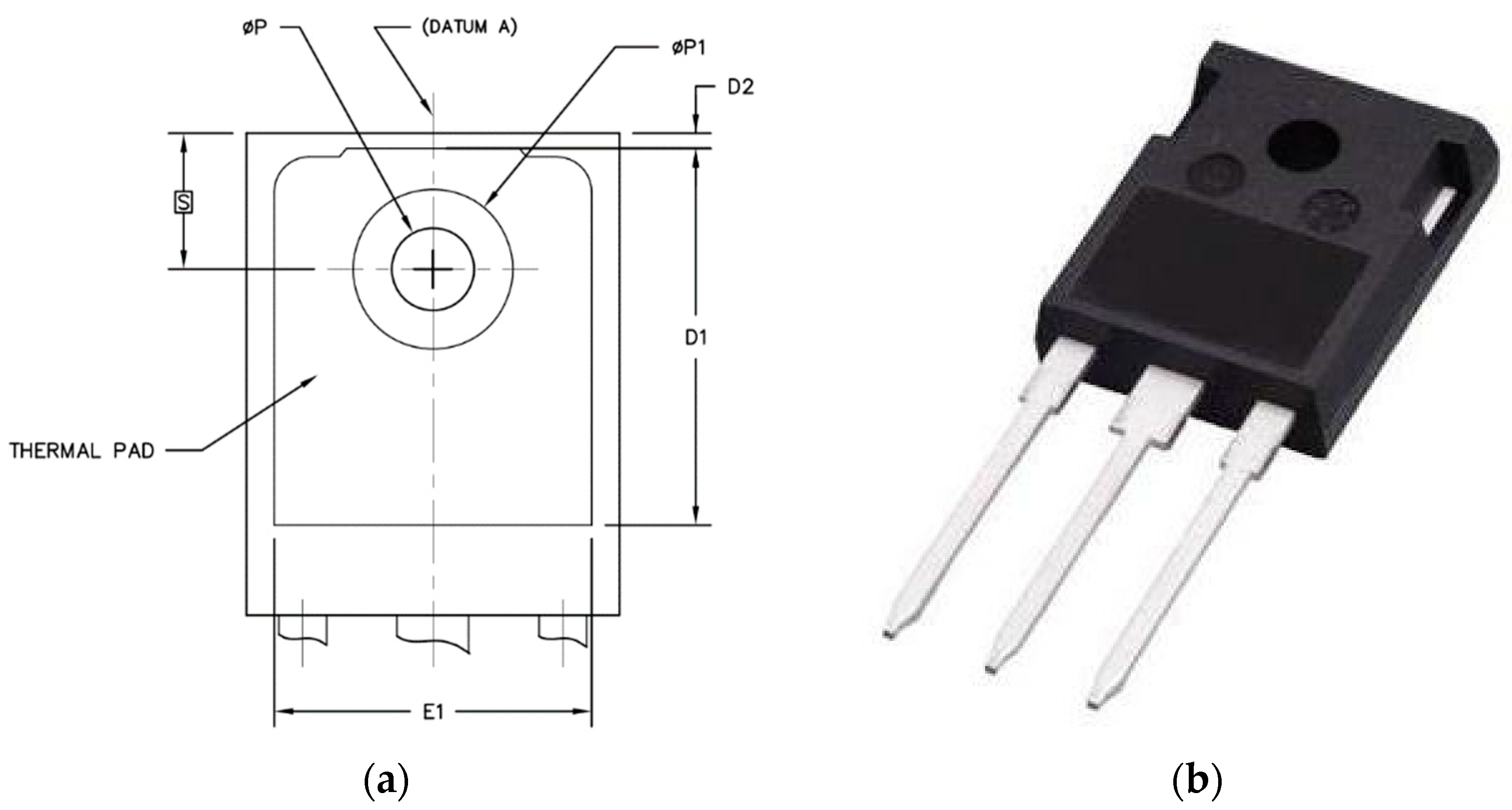
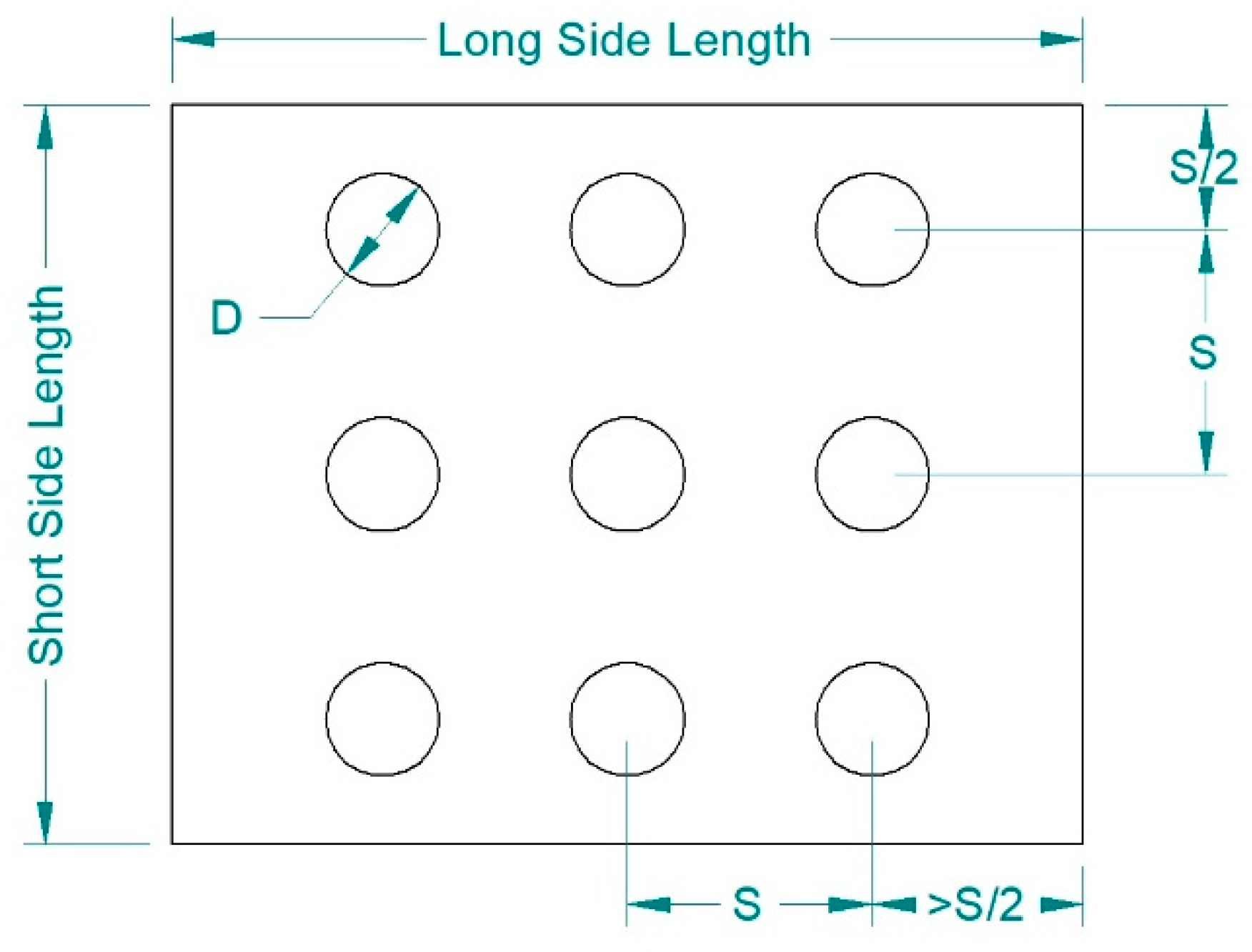
2.1. Air Jet Impingement Plate Design Procedure

An air jet impingement system is composed mainly of two elements, the target plate, which is usually part of the component from where the heat must be removed, and the impingement plate, which is a perforated plate from which, through its nozzles, the jets that impact with the component leave. The geometric configuration of the target plate must be modified to obtain the optimal solution based on certain criteria. In this case, the criteria are the temperature reached at the junction of the semiconductor to be cooled and the manufacturing time of the impingement plate itself through a machining process. The purpose of this geometry generation procedure is to find the field of feasible geometric configurations according to the geometrical constraints of the problem.

The first variable to be defined is the size of the impingement plate. This plate matches the measurements E1 and D1 of the TO-247 packaging specifications according to JEDEC, Figure 2a. In order to simplify the problem, it will be assumed that the hole designed to clip the component does not exist, eliminating the diameters øP and øP1. The addition of that geometric detail would imply that some jets do not take part in the heat exchange, complicating the thermal and flow calculation. The roundings of the upper corners are also eliminated, so that, by approaching the measurements to integer values, the area to be cooled has a width of 13 mm and a height of 16 mm. The impingement plate will therefore have this dimension. As the calculation method estimates the average Nusselt number, the more uniform the distribution of both heat and nozzles, the greater the precision of that method. Therefore, it has been decided to match the size of both plates.

Next, it is necessary to define two geometric parameters. The first is the diameter $D$ of the nozzles, both in range and in values. As machining is considered in the optimization, discrete values of diameter $D$ are used equal to the bits that are going to be used in the said operation. Eight drill bits have been chosen, whose values are 0.25, 0.30, 0.50, 0.63, 0.80, 1.00, 1.50, and 2.00 mm according to the Guhring company catalog [36]. The other geometric parameter that determines the generation of the geometry is the minimum spacing $S$ between nozzle centers. In order to secure the structural stiffness of the impingement plate, the minimum value is set in relation to the diameter to be $S/D\ge 2$. The maximum value of the distance between nozzles is set to be equal to the shortest side of the impingement plate in such a way that, with a single nozzle, the distance from the center of this to the edge of the plate is $S/2$. The same distance must also be respected in the case of more than one nozzle in the short side direction. It is therefore a vector of infinite values of S defined that will shape the real solutions for each diameter.

The first calculation step consists of determining the number of nozzles that can be placed for every combination of nozzle-to-nozzle spacing $S$ and diameter $D$, in the knowledge that this value must be integer so that it will be truncated to comply with the $S/D\ge 2$ criteria.

$$NozzleNumbe{r}_{shortside}=floor\left(\frac{shortsidelength}{S}\right)$$

(1)

However, with the resulting value of number of nozzles, the spacing S must change, so it will be:

$$S_{adjusted}=\frac{shortsidelength}{NozzleNumbe{r}_{shortside}}$$

(2)

The spacing will be the same in the long direction and in the short direction, therefore:

$$NozzleNumbe{r}_{longside}=floor\left(\frac{longsidelength}{S_{adjusted}}\right)$$

(3)

By using this arrangement, some space is wasted at the start and ending of the long direction. However, this improves the precision of the thermo-hydraulic calculation, as numerical correlations are usually made based on regular arrays. In Figure 3, an example configuration generated with this calculation method is shown.

The dimensionless distance between both plates, $Z/D$ is set as a fixed parameter of the value equal to three. This is because it is in the optimal heat transfer range for nozzle arrays for air jet impingement [37] and variations found in the range of $Z/D$ from $2\le Z/D\le 5$ have no special relevance [38].

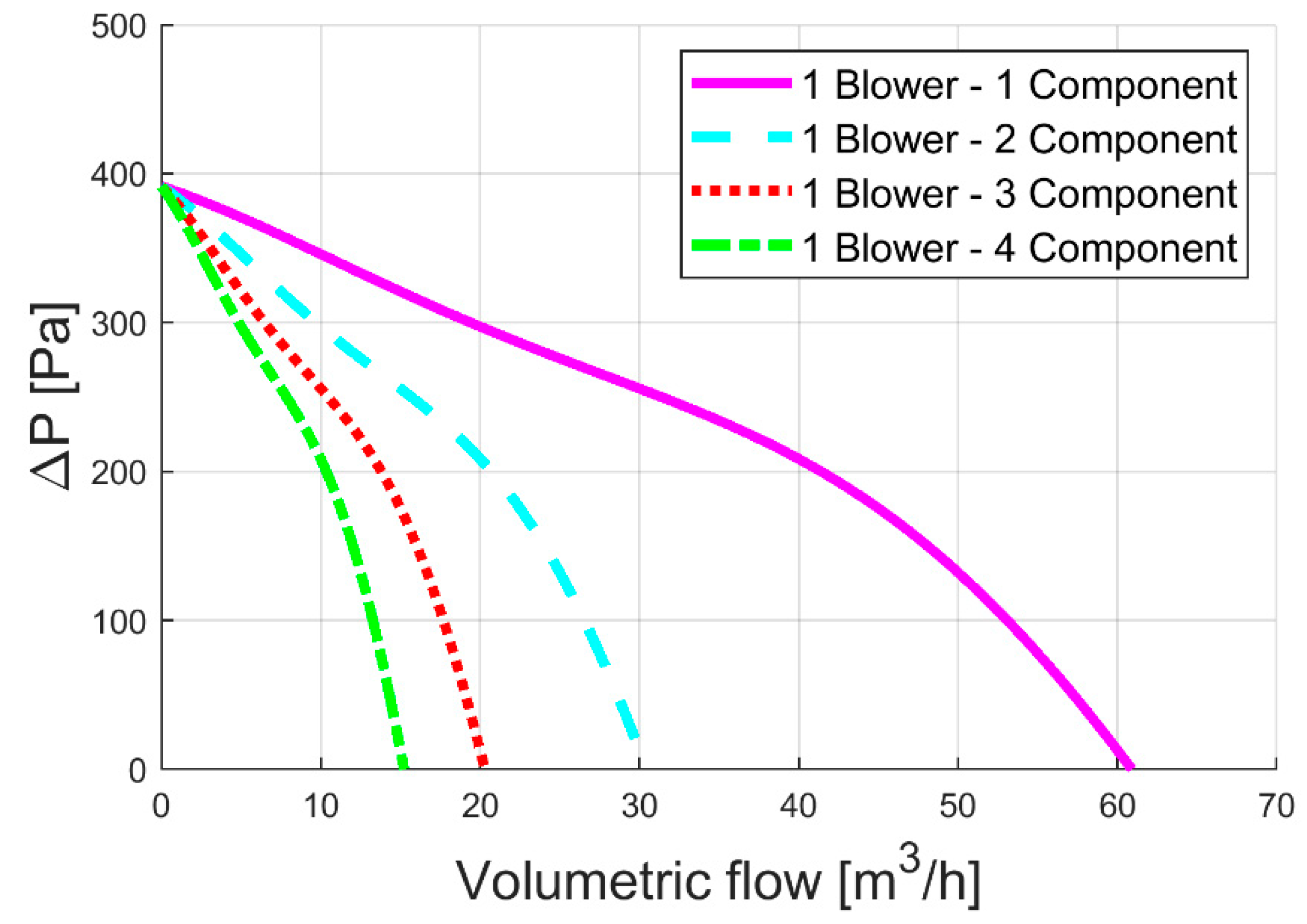
2.2. Thermo-Hydraulic Performance Calculation

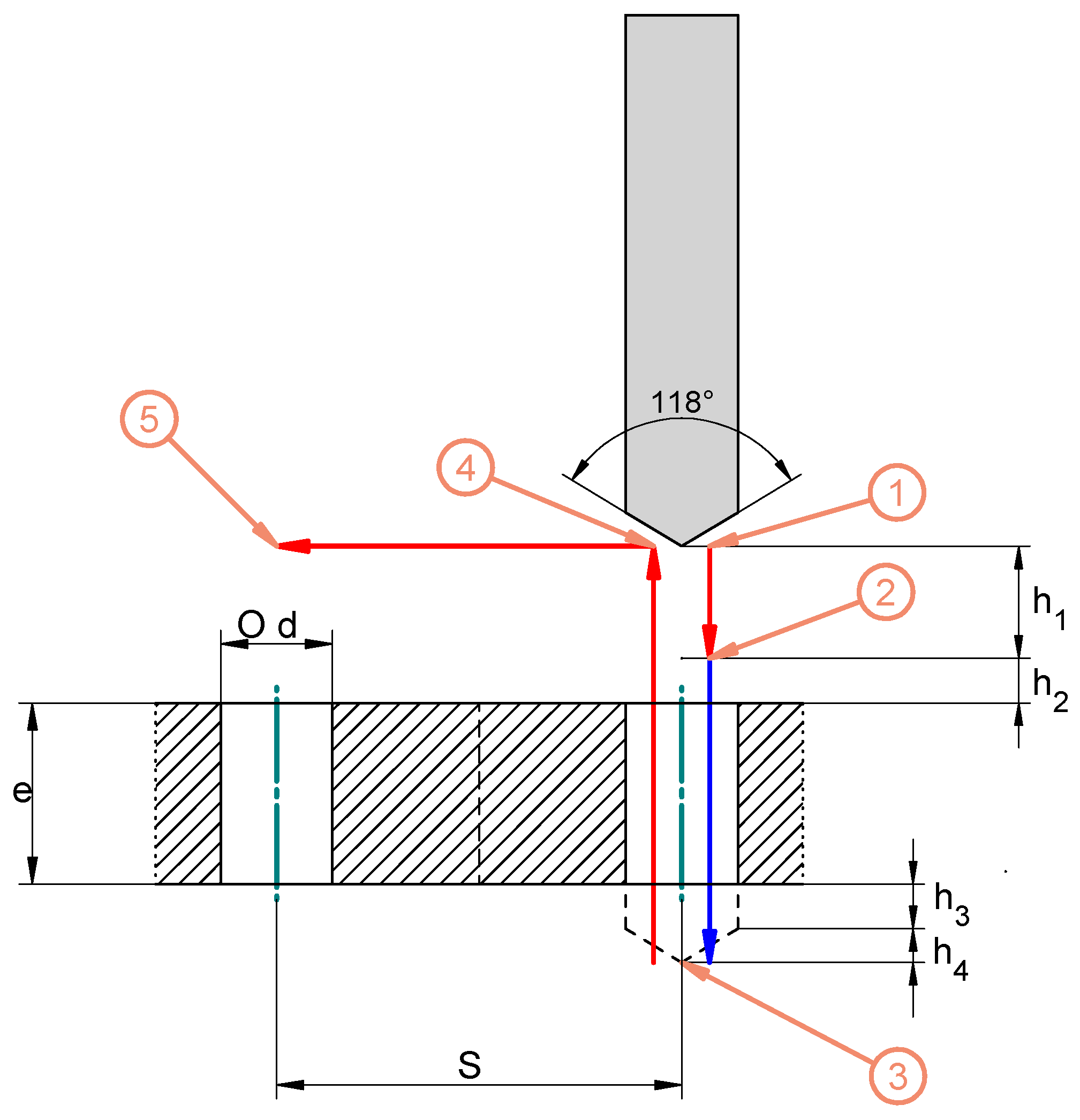
In order to evaluate the cooling capacity of the air jet impingement system, a calculation procedure has been employed to estimate the resulting flow for each impingement plate and the following cooling.

The first step is to evaluate the hydraulic operating point of the system. Every fan has a characteristic curve that relates the static pressure against the volumetric flow. Depending on the geometry of the impingement plate, the fan and the whole circuit will be operating in a point of that curve. The case study of this work consists of four discrete components, therefore the volumetric flow scale of the fan curve must be divided, and considering that all the impingement plates are identical, the dividing number must be equal to the number of components to be cooled. This step is sketched in Figure 4.

The static pressure drop that takes place in the impingement plates and has to be overcome by the fan is determined by Equation (4) proposed by Royne [39] to evaluate the pressure drop through the rectangular nozzle arrays in impingement plates.

$$\mathsf{\Delta }p=\rho Q^2\frac{8}{N^2{\pi }^2{C}_d^2{D}^4}$$

(4)

The pressure drop therefore depends on the density of the fluid $\rho$, the flow through the plate $Q$, the number of nozzles $N$, the discharge coefficient $C_d$ and the diameter of the nozzles $D$.

The discharge coefficient $C_d$ is a value that is known to vary with the Reynolds number and is the product of the contraction coefficient $C_c$ and the velocity coefficient $C_v$. These last two depend on the geometry of the nozzle and on the speed of the fluid passing through it. Due to the difficulty in determining these coefficients, Royne obtains experimentally the discharge coefficients $C_d$ for two nozzles of different plate thickness $e$ versus diameter ratio. In that case, the diameter of the holes was always 1.4 mm and the thickness of the plate was 1 and 2 mm. This discharge coefficient has theoretical limit values between 0.57 and 0.99. The first two values of

Table 1. Experimental values of discharge coefficient $C_d$. Data obtained from [39,40].

$\mathit{e}$	$\mathit{d}$	e/D	${\mathit{C}}_{\mathit{d}}$
2	1.4	1.43	0.613
1	1.4	0.71	0.582
0.021	1.4	0.015	0.57

show the diameter-thickness configurations of that study. The relationship of the $e/D$ and the $C_d$ is direct.

Given this observation, it can be thought that the minimum value of $C_d$, with a value of 0.57, would correspond to what is considered a sheet of fine thickness. According to Idelchik [40], for plates with uniformly distributed orifices, the ratio from which the fine sheet is considered is $e/D=0.015$. If this result is added to Table 1, a regression can be obtained that relates the ratio $e/D$ and the discharge coefficient, being able to calculate the $C_d$ through Equation (5). This expression can be used for the range of $e/D$ used in this study. Its values range from $e/D$ = 0.14 to $e/D$ = 1.14. In this way, estimated values can be obtained for all drill diameters selected in this case, where $e$ takes the value 1.75 mm.

$$C_d=1.8563·{10}^{-2}{\left(\frac{e}{D}\right)}^2+3.6299·{10}^{-3}\left(\frac{e}{D}\right)+5.6990·{10}^{-1}$$

(5)

Since the target and impingement plates are located far enough, $z/D=3$ and the distance between nozzle centers is $S/D>2$, it is assumed that the crossflow does not affect the individual discharge coefficient of each nozzle.

To determine the flow rate $Q$ provided by the fan, as it is implicit in the equation of the pressure drop calculation Equation (4), it has to be evaluated iteratively until convergence is reached both in $Q$ and $\mathsf{\Delta }p$. This flow rate divided between the number of nozzles $N$ of the impingement plate and given the cross-sectional area of the nozzle $A$, it is possible to estimate the air jet freestream velocity $U$ and the Reynolds number $Re$.

$$U=\frac{Q}{NA}$$

(6)

$$Re=\frac{\rho UD}{\mu }$$

(7)

To calculate the temperature of the electronic component due to the cooling caused by the impact of the jets, the correlation of Equation (8) developed by Meola [17] is used. In this equation, the average Nusselt number $N{u}_{avg}$ is related to various geometric factors of the plate, as well as the regime of the fluid passing through the nozzles. This dimensionless number relates the convective and conductive heat transfer.

$$N{u}_{avg}=0.3R{e}^{0.68}P{r}^{0.42}{\left(\frac{Z}{D}\right)}^{-0.3}{f}^{0.15}{C}_F^{0.56}$$

(8)

This expression has shown a good correlation with experiments contained in the following ranges of variables: $200<Re<$ 100,000, $1.6\le z/D\le 20$ and $0.0008\le f\le 0.2$.

The parameter $f$ is the ratio between the area with the air passage through nozzles and the area blocked by the plate and the $C_F$ is a coefficient of the friction that is the quotient of the discharge coefficient and the shape factor of the nozzle. Given the lack of knowledge of this last value, which indicates the efficiency of the nozzle, a value equal to the unity will be assumed, thus taking the $C_F$ the same value as the $C_d$. The temperature-dependent properties, $Pr$, density $\rho$ and viscosity $\mu$ needed to calculate $Re$, are taken at the temperature of the thin layer of fluid in contact with the surface, which is estimated to be the average of the temperature of the surface $T_{surf}$ of the component and the air impulsion temperature $T_{imp}$.

$$f=\frac{\pi D^2}{4S^2}$$

(9)

Once the Nusselt number has been determined, the average heat transfer coefficient of the surface to be cooled is

$$h_{avg}=\frac{N{u}_{avg}k}{D}$$

(10)

As the thermal power that the electronic components dissipate during its operation $P_{th}$ is known, the surface temperature can be calculated as:

$$T_s=T_i+\mathsf{\Delta }T$$

(11)

where the temperature increase $\mathsf{\Delta }T$ is determined by the dissipated power $P_{th}$, the average heat transfer coefficient $h_{avg}$ and the surface area to be cooled $A_{targetplate}$.

$$\mathsf{\Delta }T=\frac{P_{th}}{h_{avg}{A}_{targetplate}}$$

(12)

Finally, the component junction temperature, which is usually the limiting factor in the operation, can be estimated with the thermal resistance $R_{th}$ between the junction and the casing, whose value is usually provided by the manufacturer.

$$T_j=T_s+P_{th}{R}_{th}$$

(13)

In this temperature calculation procedure, the final solution is implicit, the reason why it will be necessary to be solved iteratively with an initial guess and making it converges.

2.3. Machining Time

For the case study, it is assumed that the manufacturing of the impingement plates will be made by the computer numerical control (CNC) machining, specifically by drilling operations on a metal plate. Depending on the nozzle size, the amount of them, and the separation between their centers, each impingement plate will have a different machining time. Since the dimensions of the impingement will be the same for all the configurations, the machining time is considered as the time used in the execution of the nozzles and the displacement between the adjacent nozzles.

The machining operations that are performed per hole are shown in Figure 5 and are described below.

The drill starts at position (1), where the machining cycle for a hole begins. Then, travels at the no-load feed speed $f_v$ a main safety distance $h_1$ until reaching position (2). This position is located at an initial safety distance $h_2$ with respect to the surface of the impingement plate. From there, the drill advances to position (3) at the cutting feed speed $f_z$, determined according to Equation (14), traveling a distance equal to the thickness of the plate $e$, the safety distance of output $h_3$ and the distance of the cone of the drill $h_3$, which assuming an angle of the drill of 118°, can be calculated by means of Equation (15).

$$f_z=\frac{f}{\frac{V_c}{0.5D}}$$

(14)

$$h_4=\frac{0.5D}{\tan \frac{118}{2}}$$

(15)

The feed speed per turn $f$ and the linear cutting speed $V_c$ are determined by the diameter and type of bit. Once the drilling has been carried out, the bit retracts vertically to position (4), coincident with position (1) at the no-load feed speed $f_v$. From there, it moves at the same speed, but in this case parallel to the plate until it is located above the location of the next nozzle (5), whose center is located at a distance $S$ from the center of the nozzle that has just been drilled.

The cycle time of each nozzle, whose movements have been described, must be multiplied by the number of nozzles to calculate the total machining time of the impingement plate.

2.4. PSO Algorithm Structure

As it is mentioned in the introduction, there are a lot of examples in the literature about how PSO algorithms are built [25,27,28].

In first place, the position $\overrightarrow{x}$ and velocity $\overrightarrow{v}$ of each particle are initialized, typically $\overrightarrow{x}$ is set to a random value and $\overrightarrow{v}$ is set to zero. In the beginning, the best position would be the actual one so the best position variable $\overrightarrow{p}$ is set equal to $\overrightarrow{x}$. Then $\overrightarrow{p}$ is evaluated by the fitness function and the result is stored as the best evaluation $p_{best}$ for each particle. Among all $p_{best}$, the best one is named the global best $g_{best}$ and the corresponding position is called $\overrightarrow{g}$.

Secondly, in the main loop, $\overrightarrow{x}$ and $\overrightarrow{v}$ are updated by the following equations:

$${\overrightarrow{v}}_{i+1}=w·v_i+c_1·r_1·\left(\overrightarrow{p}-\overrightarrow{x_i}\right)+c_2·r_2·\left(\overrightarrow{g}-\overrightarrow{x_i}\right)$$

(16)

$${\overrightarrow{x}}_{i+1}=\overrightarrow{x_i}+\overrightarrow{v_i}$$

(17)

where $c_1$ and $c_2$ are the acceleration coefficients, $w$ is the inertia weight and finally, $r_1$ and $r_2$ are random numbers between zero and one. The selection of a proper value for these coefficients would define the algorithm performance. These values can be static or can be modified following different criteria (random, time varying, adaptive) [28].

The new position is evaluated for all particles by the fitness function. If the new $\overrightarrow{x}$ has a better evaluation than $p_{best}$, $\overrightarrow{p}$ is updated and, if this evaluation is better than $g_{best}$, $\overrightarrow{g}$ is also updated.

Finally, it is necessary to determine the number of particles and the number of iterations of the PSO. The proper selection of these parameters would impact directly in the PSO performance. The bigger the number of iterations and particles, the more accurate, but at the expense of an increase of the computational cost.

3. Proposed Solution

3.1. PSO Cost Function

The solution that is proposed in this paper to the problem exposed in the previous section, consists of searching the best values for the nozzle’s diameter (D) and the nozzle to nozzle spacing and diameter ratio (S/D) by optimizing two different parameters relative to the design of the impingement plate: The target plate surface temperature and the build time. The inner temperature of the component to be cooled can be determined using the calculation procedure developed at Section 2.2 and the machining time by the method addressed in Section 2.3.

In this case, there are two functions that define the optimization process. These kinds of optimization problems are called “multi-objective optimizations”. In previous work, different approaches can be found on how to develop them: Marler et al. [41] made an overview of the different ways to handle these kinds of problems. In [42] Coello et al. the Pareto dominance is incorporated in the PSO. By contrast, Hu et al. use a dynamic neighborhood technique [43]. The other approach involves the use of a technique to scale the problem into a single objective optimization [44]. In this work the last approach is followed. Then, the cost function can be generalized as:

$$Cost={\displaystyle \sum }_{i=1}^k{w}_i·f_i\left(\overrightarrow{x}\right)$$

(18)

In this case there are two different functions, the electronic component internal temperature equation (f1) and impingement plate machining time model (f2), so rewriting (18) the cost function to solve the problem is defined:

$$Cost=w_T·Temperature+w_{Time}·Time$$

(19)

where $w_{Time}$ and $w_T$ are two coefficients whose value is defined by the designer of the cooling system depending on the approach followed, giving more importance to a low component temperature under any circumstances or to a low manufacturing cost. Usually these coefficients are defined such that:

$${\displaystyle \sum }{w}_i=1; w_i>0$$

(20)

3.2. PSO Parameters

The PSO algorithm proposed by this paper consists of a population of 50 particles, the maximum value of the range analyzed by Eberhart et al. [32] and a number of iterations of 100. Having determined these parameters, the next step is the determination of the inertia and acceleration coefficients.

Taking a look at the inertia coefficient, as it can be found in the literature, there are many ways to implement it, Nickabadi et al. [45] carried out an in-depth research about the different types of inertia weighting strategies and their performance.

Among all the adaptation mechanisms, an adaptive one has been chosen. As it can be seen in [45], “$w_{12}$” labeled inertia weight is defined by the global and the average local best fitness:

$$w=1.1-\frac{g_{best}}{{\overline{p}}_{best}}$$

(21)

On the other hand, also the acceleration coefficients $c_1$ and $c_2$ can be determined by the following different types of mechanisms, such as the linear time variation [46,47], non-linear time variation [48], or adaptive time [49,50].

One of the reasons for the use of non-constant values of $c_1$ and $c_2$ is the management of the cognitive and social effect of each particle. The cognitive component measures the impact of the best solution of the particle, while the social component deals with the best global solution. At the beginning of the PSO optimization, it is preferable to increase the impact of the cognitive components, while when reaching final values, the best strategy is to increase the social component.

In this work, the following linear time varying criteria is proposed:

$$c_1=\left(c_{1f}-c_{1i}\right)·\frac{Iter}{MaxIter}+c_{1i}$$

(22)

$$c_2=\left(c_{2f}-c_{2i}\right)·\frac{Iter}{MaxIter}+c_{2i}$$

(23)

where $c_{xi}$ is the initial value and $c_{xf}$ is the final value of each coefficient. This constant can take different values, in this case the same values as in [48], $c_{1i}$ = $c_{2f}$ = 2.5 and $c_{1f}$ = $c_{2i}$ = 0.5, are taken.

The final step is the definition of how to initialize the particles and the restriction conditions, since the input variables are D and S/D. On the one hand, as mentioned in Section 2.1, the diameter only can take eight different values, so in the beginning, this position takes one of these eight values randomly. During the optimization process, it jumps between diameter values until the end of the process. On the other hand, the S/D ratio minimum value has been fixed to two in the second section of this work. At the same time, the maximum value is defined by the plate dimensions. The short side of the plate would be the maximum distance (s) between centers (13 mm) therefore S/D takes a maximum value of 52.

4. Results and Discussion

4.1. Case Study Data

With the aim of testing the evaluation and optimization algorithm of an air jet impingement cooling system developed in this work, a solar inverter is proposed as a case study. This is a power electronics device that converts the direct current generated in the solar modules into the alternating current to be consumed or injected into the power grid. The inverters are formed by four insulated gate bipolar transistors (IGBTs), which constitute a full-bridge inverter topology.

The inefficiency of these devices is caused by the switching losses, and this energy has to be dissipated in the form of heat to preserve the integrity of the transistor and allow it to continue operating at the desired frequency and power rating. It is critical to choose the right components correctly for the upper and lower part of the bridge in order to waste the least possible energy. The better the choice, the less power will be dissipated.

A solar inverter of 1.5 kW of power with an alternating output of 230 V is taken as a reference for this calculation [51]. In a system of this type, the power dissipated by each transistor is about 7 W, and as a reference an IRG4PC40SPBF has been chosen, whose packaging is the TO-247AC shown in Figure 3 and has an internal junction-to-case resistance of 0.77 °C/W. This device has a maximum admissible joint temperature of 150 °C.

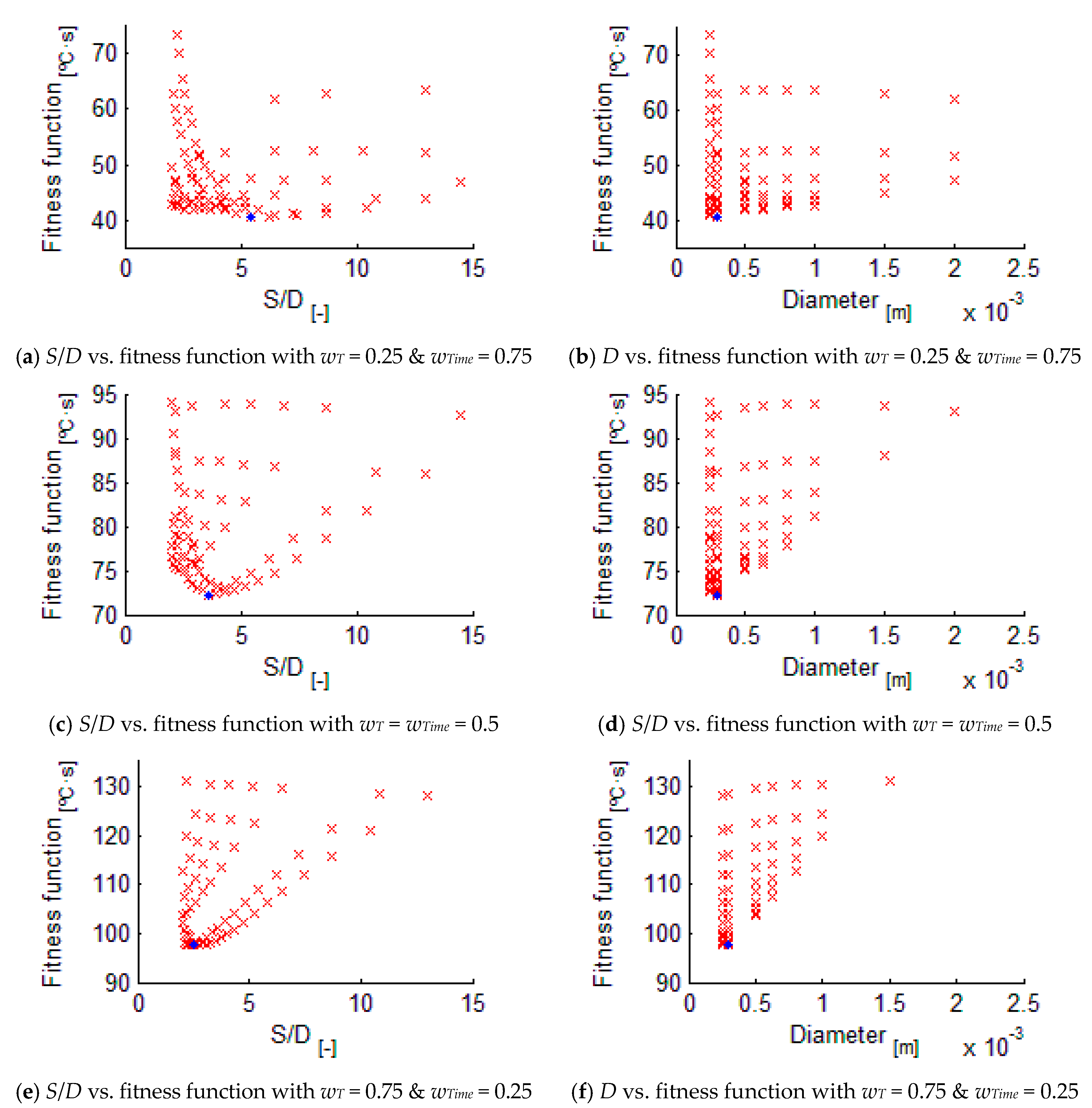
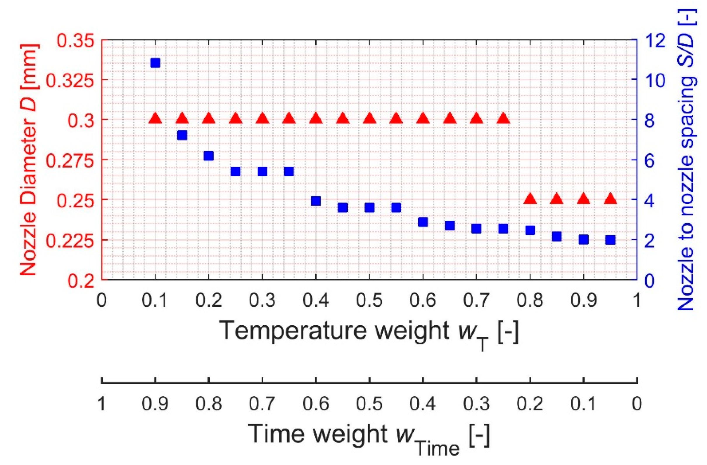
4.2. Computed Results

In order to evaluate the results that the optimization process delivers, various tests have been carried out varying the weights of the two variables that have to be optimized, both the temperature w_T and the machining time of the impingement plate w_Time.

Table 2. Solutions found by the particle swarm optimization (PSO) algorithm that satisfy the criterion specified in parameters.

Parameters	wT = 0.25 & wTime = 0.75	wT = 0.5 & wTime = 0.5	wT = 0.75 & wTime = 0.25
Diameter	0.3 mm	0.3 mm	0.3 mm
N° of Nozzles in short side	8	12	17
N° of Nozzles in long side	9	14	20
Total N° of Nozzles	72	168	340
Z	0.9 mm	0.9 mm	0.9 mm
Surface T°	137.52 °C	124.40 °C	114’95 °C
Junction T°	142.91 °C	129.79 °C	120.34 °C
Build Time	6.34 s	14.61 s	29.36 s
Nozzle center to nozzle center spacing	1.625 mm	1.083 mm	0.765 mm

shows the solutions that the geometry generation and optimization algorithm suggests.

From the left to the right of the table, the weight of the temperature of the component to be cooled increases, while the weight of the machining time decreases. As a result, variations in the proposed solutions can be observed.

The total number of nozzles is increased as the weight of the component temperature is increased. However, this increase in the number of nozzles is not coupled with a change in the diameter of these. The increase of the number of nozzles is therefore a consequence of a diminution in the separation between nozzle axes $S$, which in no case reaches the lower limit fixed in the restrictions of this case, with the ratio $S/D$ taking a minimum value of 2.55.

Regarding the distance between the impingement and the target plate, it remains constant as this parameter is directly related to the diameter of the nozzles and is adjusted to a $Z/D=3$ ratio.

Both the temperature of the semiconductor’s junction and the surface decrease as the greater number of nozzles allows more air to flow through them. For the three cases presented, the temperature reached inside the electronic component is within the acceptable range determined by the manufacturer in the steady state for the thermal loads considered. The difference in temperature between the extreme cases is slightly over 20 °C.

On the other hand, the machining time is directly influenced by the number of holes, keeping practically proportional to the number of these. The case in which the component temperature has prevailed has a manufacturing time of more than four times the case where only 25% of the weight has been assigned to that parameter. This machining time is a theoretical approach of a high-speed CNC machine without considering initial positioning or accelerations. The machining speed must be adjusted to each machine with its corresponding technical specifications and safety factors.

To observe the location of the optimal solution found by the algorithm, Figure 6 is displayed. In this figure, the three solutions exhibited in Table 2 are represented showing the fitness function, which is a combination of the variables to optimize, compared to the two independent variables, dimensionless spacing between nozzle centers $S/D$ and the diameter $D$ of these. Observing in the first place the plots of fitness function and dimensionless spacing between centers of nozzles, it can be seen how the solutions are grouped forming curves that are coincident with each discrete diameter of nozzle used in this calculation. As the weight of the temperature is increased in the target function, the value that minimizes the function, represented in blue, moves towards smaller $S/D$ values. In addition, the curvature of the solutions for each diameter is increased as this weight is increased.

Regarding the fitness function plots versus the diameter of the nozzle, it can be seen how when the weight of the machining time is greater, the solution with a lower value for each diameter is less dispersed than when this weight decreases. For the three cases, as seen in the table, the result has remained unchanged, with $D$ being in all cases of 0.3 mm.

By not observing the variation in the diameter chosen in the solutions, the number of combinations of weights of the temperature and the time of manufacture in the function of the cost to see a trend and evolution has been extended, as well as to check if the algorithm is able to choose other nozzle diameters. The results are collected in Figure 7.

In this plot it can be seen how the optimal solutions for the entire range of possible combinations of weights this problem can take, the diameter values are 0.3 mm and 0.25 mm, with the later corresponding to a temperature weight or equal than 80%. On the other hand, for the spacing between nozzle centers as the weight of the temperature increases, this spacing is reduced, but not continuously or linearly throughout the range studied.

From the analysis of these results, it seems that the choice of diameter is strongly conditioned by the flow and pressure supplied by the fan. This can also be reinforced by the fact that it is acting in a very small cooling area. A larger area can make the algorithm choose the geometries of larger nozzle diameters specially when weighting the manufacturing time.

5. Conclusions

This paper shows a procedure for calculating and optimizing an air jet impingement cooling system for power electronics components. This procedure is general for all types of electronic components with rectangular geometry and rectangular arrays of impingement nozzles of circular shape, with the minimum crossflow outlet scheme. The number of components to be cooled is adjustable, and a fan or blower with known characteristic curves must be employed.

A multi-objective PSO optimization algorithm has been developed, whose main characteristic is that, in the initialization, particles are randomly placed in a discrete field of solutions within which they will move until reaching the optimum value.

The result obtained by the PSO algorithm is in all cases the optimal, which has been compared to the calculation of all solutions individually. The amount of geometrically possible solutions is 92 for this case, which doesn’t require a lot of time to compute and evaluate all solutions. However, an increase in the dimensions of the plate, a greater number of available nozzle diameters and other variables that can be added to the problem formulation makes it advantageous to use an algorithm such as the one presented in this study, obtaining solutions in a faster way.

The weighting of the temperature and manufacturing time has been done in such a way that the factors that multiply these variables add unity. Any variation of this criterion could result in other optimal solutions, especially if the low manufacturing times are wanted, with larger nozzle diameters.

The developed algorithm for the generation and optimization of air jet impingement geometries is simple and can be easily integrated in the electronic components cooling systems design processes at the industrial level.

References

1. Lasance, C.J.M. The need for a change in thermal design philosophy. Electron. Cooling 1995, 1, 24–26. [Google Scholar]
2. Page, R.W.; Hnatczuk, W.; Kozierowski, J. Thermal Management for the 21st Century—Improved Thermal Control and Fuel Economy in an Army Medium Tactical Vehicle; SAE International: Warrendale, PA, USA, 2005. [Google Scholar]
3. Wang, Y.; Gao, Q.; Zhang, T.; Wang, G.; Jiang, Z.; Li, Y. Advances in Integrated Vehicle Thermal Management and Numerical Simulation. Energies 2017, 10, 1636. [Google Scholar] [CrossRef]
4. Chen, K.; Li, Z.; Chen, Y.; Long, S.; Hou, J.; Song, M.; Wang, S. Design of Parallel Air-Cooled Battery Thermal Management System through Numerical Study. Energies 2017, 10, 1677. [Google Scholar] [CrossRef]
5. The International Roadmap for Devices and Systems. 2017. Available online: https://irds.ieee.org/images/files/pdf/2017/2017IRDS_ES.pdf (accessed on 21 March 2019).
6. Ferranti, F.; Dhaene, T.; Russo, S.; Magnani, A.; de Magistris, M.; d’Alessandro, V.; Rinaldi, N. Parameterized thermal macromodeling for fast and effective design of electronic components and systems. In Proceedings of the 2014 IEEE 18th Workshop on Signal and Power Integrity (SPI), Ghent, Belgium, 11–14 May 2014; pp. 1–4. [Google Scholar]
7. Arik, M.; Bar-Cohen, A. Immersion cooling of high heat flux microelectronics with dielectric liquids. In Proceedings of the 4th International Symposium on Advanced Packaging Materials Processes, Properties and Interfaces (Cat. No.98EX153), Braselton, GA, USA, 18 March 1998; pp. 229–247. [Google Scholar]
8. Gould, K.; Cai, S.Q.; Neft, C.; Bhunia, A. Liquid Jet Impingement Cooling of a Silicon Carbide Power Conversion Module for Vehicle Applications. IEEE Trans. Power Electron. 2015, 30, 2975–2984. [Google Scholar] [CrossRef]
9. Smakulski, P.; Pietrowicz, S. A review of the capabilities of high heat flux removal by porous materials, microchannels and spray cooling techniques. Appl. Therm. Eng. 2016, 104, 636–646. [Google Scholar] [CrossRef]
10. Zebarjadi, M. Electronic cooling using thermoelectric devices. Appl. Phys. Lett. 2015, 106, 203506. [Google Scholar] [CrossRef]
11. Chen, X.; Ye, H.; Fan, X.; Ren, T.; Zhang, G. A review of small heat pipes for electronics. Appl. Therm. Eng. 2016, 96, 1–17. [Google Scholar] [CrossRef]
12. O’Donovan, T.S. Fluid Flow and Heat Transfer of an Impinging Air Jet. Ph.D. Thesis, University of Dublin, Dublin, Ireland, 2005. [Google Scholar]
13. Ebadian, M.A.; Lin, C.X. A Review of High-Heat-Flux Heat Removal Technologies. J. Heat Transf. 2011, 133, 110801. [Google Scholar] [CrossRef]
14. Gardon, R.; Cobonpue, J. Heat Transfer Between a Flat Plate and Jets of Air Impinging on It. In Proceedings of the International Developments in Heat Transfer, 1961–1962 Heat Transfer Conference, Boulder, CO, USA, 28 August–1 September 1961. [Google Scholar]
15. Martin, H. Heat and Mass Transfer between Impinging Gas Jets and Solid Surfaces. In Advances in Heat Transfer; Hartnett, J.P., Irvine, T.F., Eds.; Elsevier: Amsterdam, The Netherlands, 1977; Volume 13, pp. 1–60. [Google Scholar]
16. Obot, N.T.; Trabold, T.A. Impingement Heat Transfer Within Arrays of Circular Jets: Part 1—Effects of Minimum, Intermediate, and Complete Crossflow for Small and Large Spacings. J. Heat Transf. 1987, 109, 872–879. [Google Scholar] [CrossRef]
17. Meola, C. A New Correlation of Nusselt Number for Impinging Jets. Heat Transf. Eng. 2009, 30, 221–228. [Google Scholar] [CrossRef]
18. Rao, R.V.; Waghmare, G.G. Multi-objective design optimization of a plate-fin heat sink using a teaching-learning-based optimization algorithm. Appl. Therm. Eng. 2015, 76, 521–529. [Google Scholar] [CrossRef]
19. Rahimi-Gorji, M.; Pourmehran, O.; Hatami, M.; Ganji, D.D. Statistical optimization of microchannel heat sink (MCHS) geometry cooled by different nanofluids using RSM analysis. Eur. Phys. J. Plus 2015, 130. [Google Scholar] [CrossRef]
20. Zhao, J.; Huang, S.; Gong, L.; Huang, Z. Numerical study and optimizing on micro square pin-fin heat sink for electronic cooling. Appl. Therm. Eng. 2016, 93, 1347–1359. [Google Scholar] [CrossRef]
21. Kennedy, J.; Eberhart, R. Particle swarm optimization. In Proceedings of the IEEE International Conference on Neural Networks, Perth, Australia, 27 November–1 December 1995; Volume 1–6, pp. 1942–1948. [Google Scholar]
22. Heppner, F.; Grenander, U. A Stochastic Nonlinear Model for Coordinate Bird Flocks. Available online: https://www.researchgate.net/publication/216300775_A_Stochastic_Nonlinear_Model_for_Coordinate_Bird_Flocks (accessed on 21 March 2019).
23. Eberhart, R.; Kennedy, J. A new optimizer using particle swarm theory. In Proceedings of the MHS’95 Sixth International Symposium on Micro Machine and Human Science (Cat. No.95TH8079), Nagoya, Japan, 4–6 October 1995; pp. 39–43. [Google Scholar]
24. Kennedy, J.; Eberhart, R.C. A discrete binary version of the particle swarm algorithm. In Proceedings of the 1997 IEEE International Conference on Systems, Man, and Cybernetics. Computational Cybernetics and Simulation, Orlando, FL, USA, 12–15 October 1997; pp. 4104–4108. [Google Scholar]
25. Kennedy, J.; Spears, W.M. Matching algorithms to problems: An experimental test of the particle swarm and some genetic algorithms on the multimodal problem generator. In Proceedings of the 1998 IEEE International Conference on Evolutionary Computation Proceedings. IEEE World Congress on Computational Intelligence (Cat. No.98TH8360), Anchorage, AK, USA, 4–9 May 1998. [Google Scholar]
26. Kennedy, J. Probability and dynamics in the particle swarm. In Proceedings of the 2004 Congress on Evolutionary Computation (IEEE Cat. No.04TH8753), Portland, OR, USA, 19–23 June 2004. [Google Scholar]
27. Kennedy, J. Small worlds and mega-minds: Effects of neighborhood topology on particle swarm performance. In Proceedings of the Small Worlds and Mega-Minds: Effects of Neighborhood Topology on Particle Swarm Performance, Washington, DC, USA, 6–9 July 1999. [Google Scholar]
28. Fang, H.; Chen, L.; Shen, Z. Application of an improved PSO algorithm to optimal tuning of PID gains for water turbine governor. Energy Convers. Manag. 2011, 52, 1763–1770. [Google Scholar] [CrossRef]
29. Zulueta, E.; Kurt, E.; Uzun, Y.; Lopez-Guede, J.M. Power control optimization of a new contactless piezoelectric harvester. Int. J. Hydrogen Energy 2017, 42, 18134–18144. [Google Scholar] [CrossRef]
30. Hong, W.-C. Chaotic particle swarm optimization algorithm in a support vector regression electric load forecasting model. Energy Convers. Manag. 2009, 50, 105–117. [Google Scholar] [CrossRef]
31. Javaid, N.; Ullah, I.; Akbar, M.; Iqbal, Z.; Khan, F.A.; Alrajeh, N.; Alabed, M.S. An Intelligent Load Management System with Renewable Energy Integration for Smart Homes. IEEE Access 2017, 5, 13587–13600. [Google Scholar] [CrossRef]
32. Eberhart, R.C.; Shi, Y.H. Particle swarm optimization: Developments, applications and resources. In Proceedings of the 2001 Congress on Evolutionary Computation (IEEE Cat. No.01TH8546), Seoul, Korea, 27–30 May 2001. [Google Scholar]
33. Epitropakis, M.G.; Plagianakos, V.P.; Vrahatis, M.N. Evolving cognitive and social experience in Particle Swarm Optimization through Differential Evolution: A hybrid approach. Inf. Sci. 2012, 216, 50–92. [Google Scholar] [CrossRef]
34. Suresh, K.; Ghosh, S.; Kundu, D.; Sen, A.; Das, S.; Abraham, A. Inertia-Adaptive Particle Swarm Optimizer for Improved Global Search. In Proceedings of the 2008 Eighth International Conference on Intelligent Systems Design and Applications, Kaohsiung, Taiwan, 26–28 November 2008. [Google Scholar]
35. International Rectifier TO-247AC Package Outline Drawing. Available online: http://www.irf.com/package/outline/po_to247ac.pdf (accessed on 28 January 2019).
36. Guhring Guhroguía Brocas. Available online: https://www.guhring.es/Archivos/guias/84.pdf (accessed on 7 February 2019).
37. Xing, Y.; Spring, S.; Weigand, B. Experimental and Numerical Investigation of Heat Transfer Characteristics of Inline and Staggered Arrays of Impinging Jets. J. Heat Transf. 2010, 132, 092201. [Google Scholar] [CrossRef]
38. Atalla, M.A.M. Experimental Investigation of Heat Transfer Characteristics from Arrays of Free Impinging Circular Jets and Hole Channels. Ph.D. Thesis, Otto-von-Guericke-Universität, Magdeburg, Germany, 2005. [Google Scholar]
39. Royne, A.; Dey, C.J. Effect of nozzle geometry on pressure drop and heat transfer in submerged jet arrays. Int. J. Heat Mass Transf. 2006, 49, 800–804. [Google Scholar] [CrossRef]
40. Idelchik, I.E. Handbook of Hydraulic Resistance; Hemisphere Publishing Corp.: Washington, DC, USA, 1986; p. 662. [Google Scholar]
41. Marler, R.T.; Arora, J.S. Survey of multi-objective optimization methods for engineering. Struct. Multidisc. Optim. 2004, 26, 369–395. [Google Scholar] [CrossRef]
42. Coello, C.A.C.; Pulido, G.T.; Lechuga, M.S. Handling multiple objectives with particle swarm optimization. IEEE Trans. Evol. Comput. 2004, 8, 256–279. [Google Scholar] [CrossRef]
43. Multiobjective Optimization Using Dynamic Neighborhood Particle Swarm Optimization–IEEE Conference Publication. Available online: https://ieeexplore.ieee.org/abstract/document/1004494 (accessed on 1 March 2019).
44. Marler, R.T.; Arora, J.S. The weighted sum method for multi-objective optimization: New insights. Struct. Multidisc. Optim. 2010, 41, 853–862. [Google Scholar] [CrossRef]
45. Nickabadi, A.; Ebadzadeh, M.M.; Safabakhsh, R. A novel particle swarm optimization algorithm with adaptive inertia weight. Appl. Soft. Comput. 2011, 11, 3658–3670. [Google Scholar] [CrossRef]
46. Arumugam, M.S.; Chandramohan, A.; Rao, M.V.C. Competitive approaches to PSO algorithms via new acceleration co-efficient variant with mutation operators. In Proceedings of the Sixth International Conference on Computational Intelligence and Multimedia Applications (ICCIMA’05), Las Vegas, NV, USA, 16–18 August 2005. [Google Scholar]
47. Ratnaweera, A.; Halgamuge, S.K.; Watson, H.C. Self-organizing hierarchical particle swarm optimizer with time-varying acceleration coefficients. IEEE Trans. Evol. Comput. 2004, 8, 240–255. [Google Scholar] [CrossRef]
48. Ghasemi, M.; Aghaei, J.; Hadipour, M. New self-organising hierarchical PSO with jumping time-varying acceleration coefficients. Electron. Lett. 2017, 53, 1360–1361. [Google Scholar] [CrossRef]
49. Suganthan, P.N. Particle swarm optimiser with neighbourhood operator. In Proceedings of the 1999 Congress on Evolutionary Computation-CEC99 (Cat. No. 99TH8406), Washington, DC, USA, 6–9 July 1999. [Google Scholar]
50. Yamaguchi, T.; Yasuda, K. Adaptive particle swarm optimization—Self-coordinating mechanism with updating information. In Proceedings of the 2006 IEEE International Conference on Systems, Man and Cybernetics, Taipei, Taiwan, 8–11 October 2006. [Google Scholar]
51. Chou, W. Choose Your IGBTs Correctly for Solar Inverter Applications. Available online: https://www.infineon.com/dgdl/524pet0808.pdf?fileId=5546d462533600a4015356926b322b5f (accessed on 21 March 2019).
Figure 1. (a) Side view of a single air jet flow scheme, regions and fluid behavior adapted from [12]; (b) top view scheme showing the difference between the three kinds of crossflows. The arrows show the spent flow direction.
Energies 12 01627 g001
Figure 2. (a) Technical drawing of TO-247AC package according to JEDEC. Obtained from [35]; (b) perspective picture of the package.
Energies 12 01627 g002
Figure 3. Example of the geometry generated by the described algorithm, with three nozzles in the short direction, three nozzles in the long direction, same spacing between nozzles in both directions and minimum separation between the center of any nozzle and the edge of impingement plate of S / 2 .
Energies 12 01627 g003
Figure 4. Original blower (ebm-papst RL65-21/12H) flow versus static pressure curve (-) and the corresponding curves for systems with two (- -), three (· ·) and four (-·-) components to be cooled by the blower.
Energies 12 01627 g004
Figure 5. Diagram of the machining process of the nozzles by drilling and the distances and measurements involved in the calculation of the manufacturing time. The trajectories in red are at the rapid speed f v and in blue at the cutting speed f z .
Energies 12 01627 g005
Figure 6. Spatial representation of the fitness function with respect to the independent variables S / D and D .
Energies 12 01627 g006
Figure 7. Results of the solution, nozzle diameter D and dimensionless spacing between nozzle centers S / D for the variation of the weight of the temperature in the cost function.
Energies 12 01627 g007