Abstract
The powertrain efficiency deeply affects the performance of off-road vehicles like wheel loaders in terms of fuel economy, load capability, smooth control, etc. The hydrostatic transmission (HST) systems have been widely adopted in off-road vehicles for providing large power density and continuous variable control, yet using relatively low efficiency hydraulic components. This paper presents a hydrostatic-mechanical power split transmission (PST) solution for a 10-ton wheel loader for improving the fuel economy of a wheel loader. A directly-engine-coupled HST solution for the same wheel loader is also presented for comparison. This work introduced a sizing approach for both PST and HST, which helps to make proper selections of key powertrain components. Furthermore, this work also presented a multi-domain modeling approach for the powertrain of a wheel loader, that integrates the modeling of internal combustion (IC) engine, hydraulic systems, mechanical transmission, vehicle(wheel) dynamics, and relevant control systems. In this modeling, an engine torque evaluation method with a throttle position control system was developed to describe the engine dynamics; a method to express the hydraulic loss of the axial piston hydraulic pump/motor was developed for modeling the hydraulic transmission; and a vehicle velocity control system was developed based on altering the displacement of a hydraulic unit. Two powertrain models were developed, respectively, for the PST and HST systems of a wheel loader using MATLAB/Simulink. The simulation on a predefined wheel loader drive cycle was conducted on both powertrain models to evaluate and compare the performance of wheel loader using different systems, including vehicle velocity, hydraulic displacement control, hydraulic torque, powertrain efficiency, and engine power consumption. The simulation results indicate that the vehicle velocity controller developed functions well for both the PST and HST systems; a wheel loader using the proposed PST solution can overall save about 8% energy consumption compared using an HST solution in one drive cycle. The sizing method and simulation models developed in this work should facilitate the development of the powertrains for wheel loaders and other wheeled heavy vehicles.
1. Introduction
The energy consumptions of off-road vehicles such as wheel loaders mainly depend on the energy efficiency of their transmission systems, which usually adopts continuous variable transmission (CVT) to improve the comfort. Current technologies allow following CVT solutions: hydrodynamic transmission (torque converter), hydrostatic transmission (HST) (hydraulic pump/motor), mechanical transmission, and electric transmission. The hydrodynamic and hydrostatic solutions have been commonly used in off-road vehicle applications when comprehensively considering efficiency, power density, speed range, cost, etc. However, the efficiency of an HST is still relatively low due to the repeated energy conversion, and the hydrodynamic transmission usually can only achieve high efficiency at high speed scenarios [1,2]. It has been realized that a satisfying efficiency performance cannot be achieved by a pure CVT. Therefore, researchers have proposed a novel type of transmission, usually named as power split transmission [3,4]. In a power split transmission (PST), the transmitted power is shared by two different transmission paths: a mechanical path with normally high efficiency, and a hydrostatic or hydrodynamic path for CVT. The power from the two paths will be combined through a planetary gear set. This PST has been expected to become a more efficient CVT compared to a directly coupled CVT. Blake et al. studied different power–split architecture: input coupled, output coupled, and complex solutions, which show advantage in heavy vehicle applications [5]. Specifically for the wheel loader application, Nilsson et al. presented a multi-mode hydrostatic-mechanical power split transmission, which achieved at least 15% better fuel saving potential than the present torque converter solution [6]. Liu et al. replaced the existing torque converter with a hydrodynamic-mechanical PST for a wheel loader, which shows 3.38% fuel saving rate [7].
In order to evaluate the performance of newly proposed powertrain architecture, researchers also developed various modeling methods particularly for the hydraulic system and internal combustion (IC) engine. For analyzing the efficiency of HST for off-road vehicles, Comellas et al. applied constant parameters to linear and quadratic coefficients, respectively, for the hydraulic flow and pressure loss [2]; Schulte developed hydraulic pump/motor flow expression as a function of input current to the control servo-valve and introduced a pressure dependent coefficient to evaluate flow leakage [8]. When studying the fuel consumption of urban buses using PSTs, Macro and Rossetti modeled the behavior of the hydraulic units by applying to an ideal unit two loss coefficients: friction coefficient for pressure loss and orifice coefficient for flow leakage, which were expressed in polynomial functions of unit speed, load pressure and displacement position [9]. For engine modeling, apart from developing an engine efficiency map from experimental testing [7,9,10], Nillson et al. expressed engine torque as a function of engine speed and fuel injection using quadratic efficiency model when predicting the fuel potential of power split CVT for a wheel loader [6]. As for the system modeling tool, Kim et al. created subsystem models for all function components of a hydrostatic powertrain and integrated them as a whole system model using MATLAB/Simulink, which was experimentally validated when analyzing the energy flow of a wheel loader [10]. Besides, commercial software Amesim with embedded time-dependent analytical equations for a hydraulic, pneumatic, thermal, electric, or mechanical system has also been frequently adopted to investigate powertrains as multi-domain systems [9,11].
There is more literature on investigating the efficiency and control strategy of heavy vehicles’ powertrains by means of simulations [12,13]. However, these works above rarely reveal the design procedure of the transmission system, particularly when it involves hydraulic components. Cundiff introduced a sizing process for a hydrostatic powertrain of a harvester focusing on the sizing of hydraulic units, in which the gear ratios of mechanical transmission were pre-selected based on some off-the-shelf products [14]. Although such an approach may facilitate the sizing process, a sizing method that combines hydraulic units and mechanical components should be able to recommend more accurate and flexible options.
The purpose of this work was to design and analyze a hydrostatic-mechanical PST for a wheel loader given a set of design specifications and assumptions. One contribution of this work is to present a fundamental design procedure which included sizing and selections of key hydraulic and mechanical components. For comparison, this work also presented a design solution to a directly-engine-coupled HST for the same wheel loader. Section 3 will detail the sizing procedure of the key components of the HST and PST. Another contribution of this work is to introduce a multi-domain modeling approach to describe the powertrain system of a wheel loader which integrates combustion engine system, hydraulic system, wheel dynamics, and mechanical transmission, wheel dynamics, and control systems. Section 4 will detail the modeling development, which includes the mathematical modeling for general physics and unique modeling techniques comparing to other state-of-the-art modeling methods. Based on the proposed modeling approach, this work developed two powertrain models, respectively, for designed PST and HST systems, and simulations were conducted to predict and compare their performances under specified operation conditions in Section 5.
2. Powertrain Schematic
Figure 1 shows basic schematics of HST and PST powertrains for a wheel loader. In this project, an output coupled PST operation mode was adopted for wheel loader PST design. An HST starts out with the combustion engine (CE), which first serially coupled with a hydraulic system and then a mechanical transmission set in sequence. The hydraulic system includes two variable displacement pump/motors: one as pump Unit 1 to directly transmit the engine power through the hydraulic lines and another as motor Unit 2 to transmit hydraulic power to following mechanical gear sets. The mechanical transmission includes a two-stage gearbox allow the gear ratio to shift between two levels (iI and iII) for different load situations and an axle gear set with fixed ratio iaxle to adapt required wheel loader speed. In a PST powertrain, the engine power was firstly transmitted to a planetary gear set through the input shaft. The planetary gear set allows the input shaft drive the carrier C and divide the input power into two parts: one ring gear R to Unit 1 transmits the power through the hydraulic path by a gear set with ratio i1; another from sun gear S to two-stage gearbox through the mechanical path. In order to combine the split power, the Unit 2 was connected the sun gear shaft by the gear set with ratio i2. In this work, the hydraulic transmission of PST shared the same circuit (component size may be different) with the one of HST, as shown in Figure 2. Moreover, the PST and HST powertrain adopted the same gear ratio settings for both two-stage gearbox and axle gear set.
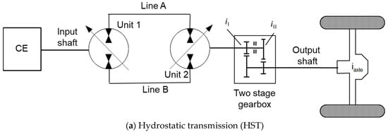
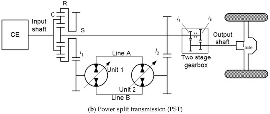
Figure 1.
Schematics of the proposed wheel loader powertrains.
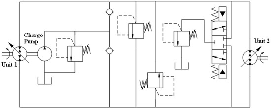
Figure 2.
Hydraulic circuit of the wheel loader powertrain.
3. Powertrain Sizing
3.1. Maximum Load Requirements
Table 1 lists the all design specifications and assumptions for wheel loader powertrain design.

Table 1.
Wheel loader design specifications and assumptions [14].
The powertrain for a wheel loader (as shown in Figure 3) should be able to handle the maximum applied wheel torque. The following three possible scenarios during the wheel loader operation were investigated here to find the maximum torque applied to the wheels:
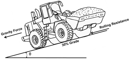
Figure 3.
Wheel loader with payload on a 30% slope.
- Driving on flat asphalt road accelerating to maximum speed;
- Driving on flat ground of soil with maximum pulling effort;
- Driving on a maximum climbing slope of soil road.
The load torque applied to the wheel loader TW can be calculated based on following equations:
Here, R represents the rolling resistance along the travel path, which can be asphalt road or soil ground. The vehicle acceleration aveh is assumed to be constant for its calculation in this sizing study. The three scenarios are subjected to corresponding operation conditions shown in Table 2, which also shows the resulting wheel torque values, which are, respectively, represented by MI, MII, MIII. It can be found that the maximum applied wheel load occurs in scenario III, which is 30,446 Nm.
Table 2.
Possible operation scenarios with maximum wheel load.
3.2. HST Sizing
The design of the HST drivetrain involves with the sizing and selection of hydraulic Unit 1 and Unit 2’s displacement (Vi1 and Vi2) and gear ratio for the two-stage gearbox. In order to facilitate gear ratio sizing, the gearbox ratio ig and the axle ratio iaxle can be combined into one ratio:
3.2.1. Unit 2 and Gearbox Sizing
The speed norm and the torque norm will be combined to size Unit 2 and gearbox.
(1) Speed Norm
In the norm of speed requirements, the maximum low speed gear ratio ilow should be able to handle the vehicle’s shifting speed vshift and the maximum high-speed gear ratio ihigh should help to reach a wheel load speed vmax. Moreover, the speed norm also requires Unit 2 run at its maximum operating speed. The gear ratios should be subject to following equation:
(2) Torque Norm
The torque transmitted to wheel from Unit 2 can be calculated using Equation (4):
In the norm of torque requirements, the minimum low speed gear ratio ilow should help to provide a wheel torque of 30,446 Nm, and the minimum high-speed gear ratio ihigh should help to provide a wheel torque of 4732 Nm, according to Table 3.
Table 3.
HST Unit 2 selection lookup table [15].
Based on above sizing equations, Unit 2 selection lookup table can be developed. This work selected Danfoss Series 90 variable displacement pump/motors for Units 1 and 2. The ones with 75 cc and 100 cc displacement meet design requirements (min. ilow < max. ilow; min. ihigh< max. ihigh). To avoid extra costs and power wasting, the 75 cc machine is selected as HST Unit 2. Accordingly, the low speed gear ratio ilow could be set as 85 the high-speed gear ratio ihigh could be set as 17. Since the axle gear ratio is specified as 4.25, the low speed gear ratio iI and high speed 2 gear ratio iII of two-stage gearbox is, respectively, set as 20 and 4.
3.2.2. Unit 1 Sizing
The sizing of HST Unit 1 displacement V1 should be able to handle all 90 kW from engine and V1 should be at least:
(1) Speed Norm
Therefore, a 75 cc Danfoss Series 90 variable displacement pump should be sufficient [16]. The information of key components of wheel loader HST is included in Table 4.
Table 4.
Major components of wheel loader HST.
3.3. PST Sizing
3.3.1. Planetary Gearing Sizing
In this work, the PST powertrain used the same gear ratios for two-stage gearbox. The design of the PST drivetrain involves with the sizing and selection of hydraulic Unit 1 and Unit 2’s displacement (Vi1 and Vi2), the gear ratio io for the planetary gear set and gear ratios of two power-split gear sets (i1 and i2). A planetary gear ratio is subjected to following equation:
The vehicle speed at full mechanical point (ns = 0) helps to determine the planetary gear ratio, and it can be calculated using Equation (7):
3.3.2. Unit 2 and Power Split Gear 2 Sizing
The sizing of Unit 2 displacement V2 and gear ratio i2 sizing for PST was subjected to following sizing norms:
- (1)
- Speed Norm:
- (2)
- Torque Norm:
Then based on above sizing equations, a Unit 2 selection lookup table was built up in Table 5. Note that the sizing of PST still selected the Danfoss Series 90 variable displacement machines for both Units 1 and 2.
Table 5.
PST Unit 2 selection lookup table [15].
It can be found that only the ones with 75.0 cc and 100.0 cc maximum displacement meet design requirements (i2min < i2max). To avoid extra costs and power wasting, the 75 cc Danfoss Series 90 machine is selected as PST Unit 2. Accordingly, this work selects 1 for the gear ratio i2 (0.93 < i2 < 1.08).
3.3.3. Unit 1 and Power Split Gear 1 Sizing
The sizing of Unit 1 displacement V1 and gear ratio i1 sizing for PST was subjected to following sizing norms:
- (1)
- Speed Norm:
- (2)
- Torque Norm:
Then based on above sizing equations, the PST Unit 1 displacement V1 and gear ratio i1 can be selected using Table 6.
Table 6.
PST Unit 1 selection lookup table [16].
It was found available displacement machine all satisfies design requirements (min. i1< max. i1) and the 42 cc variable displacement machine was selected. Accordingly, the gear ratio i1 was set as 1.4 (1.2 < i2 < 1.74). Therefore, information of major components of wheel loader PST is included in Table 7.
Table 7.
Major components of wheel loader HST.
4. Modeling Development
The HST and PST powertrains proposed in Section 3 belong to multi-domain systems that include combustion engine, hydraulic system, mechanical transmission, vehicle dynamics, and control system. An effective powertrain model should describe the physics of each domain and integrate them together as a whole.
4.1. Engine Model
The engine shaft dynamics is subjected to following equation:
where JE is the engine rotor’s moment inertia; TE, TL, and Tf, respectively, represents torque from combustion, engine load torque, and friction torque.
The engine torque against different operation conditions can be acquired using an engine map [10]. This work developed a curve of engine torque TE_100% at full throttle against different engine speed based on the experimental data provided by Purdue University [17], as shown in Figure 4.
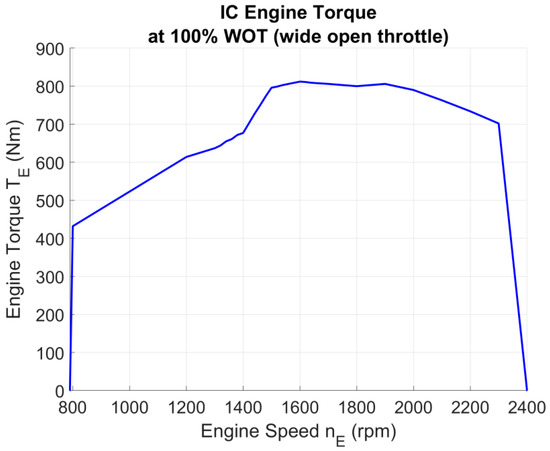
Figure 4.
Internal combustion (IC) engine torque curve at 100% wide open throttle.
This modeling assumes the engine torque at certain speed linearly changes with throttle position βE (%), so the engine torque TE can be evaluated using following equation:
The throttle position is typically modeled as preset condition of engine model [10]. This work created a proportional–integral–derivative (PID) controller to maintain the engine running at a target speed and the throttle position was modeled as the direct output of this engine speed controller, as shown in Figure 5. Note that a first order transfer function with time constant tE was utilized to describe the dynamic response of throttle position control.
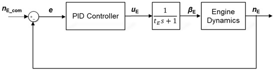
Figure 5.
Engine Speed Controller.
As for the engine friction torque, this model assumes the Tf is linearly dependent on engine speed with a linear coefficient kf, which can be expressed in Equation (14):
4.2. Hydraulic System Model
The hydraulic system shown in Figure 2 can be described by following equations.
Hydraulic Unit 1 and Unit 2 dynamics:
where J1 and J2 represent the moment inertia of Unit 1 and Unit 2; T1 and T2 represent the torque transmitted to Unit 1 directly from engine and output torque from Unit 2; the swash plate angle position(displacement percent) β1 and β2 of Unit 1 and Unit 2 both range from −100% to 100% (positive value means the unit runs as pump, otherwise as motor) and they will be controlled by feeding back value of vehicle velocity to keep the wheel loader running at commanded velocity; pA and pB represents pressure of line A and Line B, which can be determined by following equations.
Hydraulic transmission line pressure buildup equations:
where K is the bulk modulus of hydraulic fluid; VA and VB represent the fluid volume stored in hydraulic line A and B; Qr and Qc represents flow through the relief valve and check valve, which can be calculated using the following equations.
(3) High pressure relief valve and low pressure check valve’s characteristics [13]:
where Kr and Kc represent the flow coefficient of relief valves and check valves; pr and pc are threshold pressure settings of relief valves and check valves and are, respectively, set as 400 bar and 20 bar in this work.
The key inputs to above hydraulic system modeling are the torque loss (Ts1 and Ts2) and flow loss (Qs1 and Qs2) of Unit 1 and Unit 2. Some study may use a constant value [9] or a pressure-dependent function [10] to describe the torque and volumetric efficiency. Instead of using one constant for efficiencies in sizing of Section 3, this modeling developed expressions (as expressed in Equation (19)) for torque loss and flow loss at certain combination of pump/motor speed, differential pressure, and swash plate angle position by implementing fifth-order polynomial interpolations of the testing data of an axial piston machine [17].
4.3. Mechanical Transmission Model
The torque and speed transmitted through mechanical gearings are subjected to following equations.
- (1)
- For HST:
- (2)
- For PST:
Here, TW and TL represent the torque applied to the wheels and the load torque to the engine shaft.
4.4. Vehicle Dynamics and Control
The vehicle dynamics is subject to following equations:
The calculated vehicle velocity vveh will be feedback to a brake controller to keep the vehicle running at commanded velocity vcom by adjusting the displacement (β1 and β2 of either hydraulic unit, as shown in Figure 6. A sequential state flow algorithm with a selection parameter Sβ ensures that Units 1 and 2 will not control the velocity simultaneously. Note that the first order transfer functions with time constant t1 and t2 were utilized to describe the dynamic response of swash plate angle control.
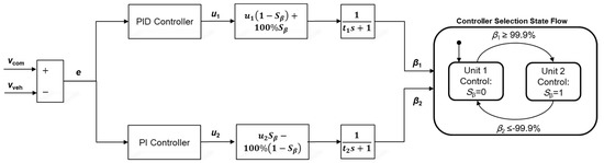
Figure 6.
Wheel loader velocity controller.
5. Simulation Analysis
In this study, the powertrain models were developed based on a MATLAB/Simulink programming environment. This allows developers to create subsystem models for the powertrains’ functional parts and then link them together as a model for the whole powertrain systems. The Simulink models for HST and PST powertrains were developed as shown in Figure 7. The HST and PST models share the same subsystems for modeling combustion engine, vehicle dynamics, and two-stage gearbox. The hydraulic modules in HST and PST adopt the same architecture and only use different parameter setting for Unit 1. The modules of planetary gearbox and power split gearing sets have been specifically created for the PST powertrain model. The HST and PST powertrain models will run at the same operating conditions, including vehicle velocity profiles, gear selection profiles, slope grade, cargo mass, rolling resistance, and pulling effort, as shown in Figure 8 and Figure 9.
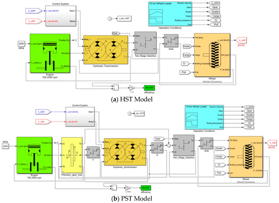
Figure 7.
MATLAB/Simulink models of wheel loader powertrains.
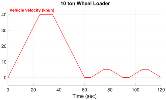
Figure 8.
Commanded wheel loader motion profile.
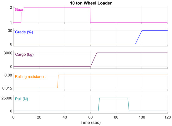
Figure 9.
Wheel loader operation condition profiles of the predefined drive cycle.
In this study, the wheel loader was commanded to follow a predefined 2 min drive cycle. The defined drive cycle includes two phases. The commanded drive cycle starts from phase I: driving without payload. Initially, a velocity command is given to the hydrostatic units, which then bring the vehicle up to 40 km/h in 25 s. Note that the two-stage gearbox will shift from level I to level II when the vehicle reaches the shifting velocity 10 km/h. The wheel loader will keep traveling on the asphalt road at 40 km/h for about 10 s, and then the wheel loader is controlled to slow down to standstill in 25 s when it enters the soil ground field.
After 5 s standstill preparation for cargo loading: Shifting two-stage gearbox to level I, the drive cycle enters into phase II: driving with payload. The wheel loader is firstly commanded to bring the vehicle up to 5 km/h in 10 s with specified maximum 25 kN pulling effort and keep driving at 5 km/h for 10 s; then it will slow down to standstill. Then the wheel loader gradually starts to climbs up on a 30% slope and unloads the 25 kN pulling effort. Lastly, the vehicle is commanded to drive on the 30% slope at 5 km/h and then slow down to standstill at 120 s to finish this drive cycle.
In this study, this simulation will analyze the following variables to evaluate and compare the performance of the wheel loader powertrains:
- Vehicle Velocity
- Hydraulic Units’ Displacement Position
- Hydraulic Torque
- Engine Power and Powertrain Efficiency
5.1. Vehicle Velocity
As shown in Figure 10, the designed HST and PST powertrains enables the wheel loader meet the speed and acceleration requirements. The wheel loader reached maximum 40 km/h in 25 s in Phase I; it also successfully worked with 25 kN pulling effort at 5 km/h and climbed up onto a 30% slope with 5 km/h in Phase II. Moreover, the designed controller successfully makes the wheel loader travels closely following the commanded velocity profile. The simulation values from the PST model seem less close to targeting velocity compared with that from the HST model.
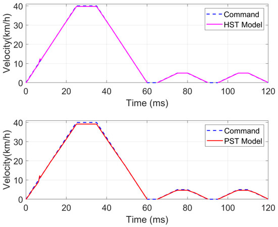
Figure 10.
Commanded vehicle speed versus actual vehicle speed.
5.2. Hydraulic Units’ Displacement Position
As shown in Figure 11, this study defines the displacement percent as positive (+) while the hydraulic unit runs as a pump and negative (—) while one runs as a motor. In a PST model, Unit 1 starts at zero displacement and ramps up as a pump to full displacement. Meanwhile, Unit 2 starts as a motor with full displacement and then de-strokes as the vehicle running faster. Once the vehicle velocity passes the switching speed of 10 km/h, the two-stage gearbox is commanded to switch to the high-speed gear ratio. This is where Unit 2 runs back to −100% displacement and Unit 1 begins to de-stroke to a point where the vehicle speed matches the commanded speed. After 35 s, the vehicle starts to slow down, Unit 2 runs from −16% displacement to −100% displacement, where Unit 1 starts to de-stroke until it reaches zero displacement and the vehicle stops. In Phase II, Unit 1 pumps to full displacement again; meanwhile, Unit 2, running as a motor, de-strokes to about −66%, until the vehicle reaches the maximum velocity 5 km/h. Then, during wheel loader climbing up 30% slope, Unit 1’s pumping displacement keeps increasing as far as the engine operates without stalling. In order to maintain 5 km/h velocity, Unit 1 operates at full displacement while Unit 2’s displacement only needs to operate at −67% of full displacement.
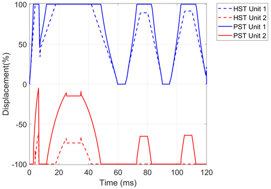
Figure 11.
The controlled displacement profiles of Units 1 and 2.
In the HST model, Unit 2’s displacement is much larger than that in the PST model at steady driving, and it de-strokes later than that in PST model. Particularly in Phase II, Unit 2 only needs to operate around 67% of full displacement in the PST model, while it kept operating at full displacement in the HST model. In a PST powertrain, the planetary gearing allows the engine power being partially transmitted to the hydraulic system, so Unit 2 can operate at a relatively smaller percent of motoring displacement.
5.3. Hydraulic Torque
Figure 12 shows the hydraulic torque output from Unit 2 throughout the drive cycle. Unlike staying constant in the HST model, the hydraulic torque in the PST model keeps changing with the vehicle speed during the acceleration or deceleration period. It can be also found that the hydraulic torque in the PST model is generally smaller than that in the HST model. Again, this is because there is some torque being transmitted through the planetary gearing in a PST powertrain, while the hydraulic system in an HST powertrain has to deal with all torque applied to the wheels.
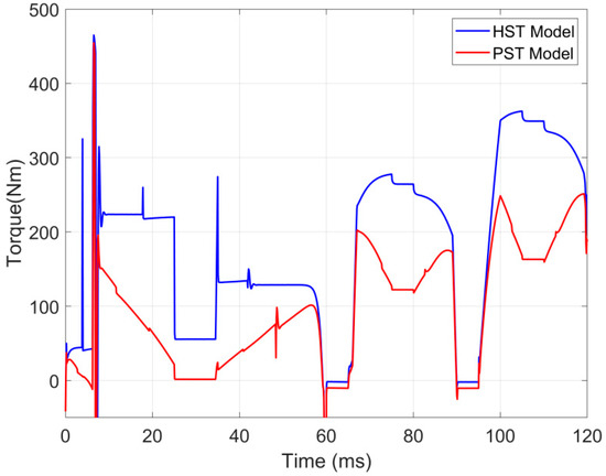
Figure 12.
Hydraulic torque of Unit 2.
5.4. Engine Power and Powertrain Efficiency
The effective power from fuel combustion of engine PE are plotted out in Figure 13. The modeled engine successfully provided the powertrain with maximum rated 90 kW, and the engine power in the PST model is generally less than that in the HST model.
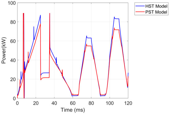
Figure 13.
Effective power from engine fuel combustion.
The efficiency of entire powertrain can be calculated using Equation (25):
Figure 14 shows the simulated efficiency results of the HST and PST powertrain. It shows that the peak efficiency value of the PST when driving at maximum speed on asphalt road and driving on 30% slope are both close to 84%. When the wheel loader decelerates on the asphalt road in Phase I, the simulated powertrain efficiency values are beyond 100%. This is because rolling resistance force in this phase is able to slow down the wheel loader at the commanded deceleration rate.
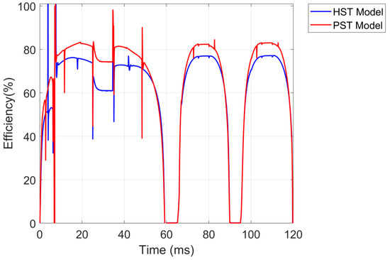
Figure 14.
Powertrain Efficiency.
Moreover, it is clear that the efficiency achieved using the PST is generally higher than using an HST, particularly when the wheel loader operates at a steady motion status. For example, when the wheel loader is driving at 5 km/h on flat soil ground, the peak efficiency of the PST powertrain is 83.5%, which is higher than the 77.7% of the HST by 7.5%.
In addition to transient efficiency plots, average powertrain efficiency for entire drive cycle was also investigated in this study, based on Equation (26):
By integrating simulated power values over time, the energy consumption through the powertrain can be obtained as shown in Table 8. It can be found that the average efficiency of the PST is 76.6%, higher than the 70.9% of the HST by about 8%.
Table 8.
Energy analysis of entire drive cycle.
6. Conclusions
The directly-coupled HST and the output-coupled PST were both properly sized and modeled. The simulations show that the design solutions meet the given design requirements. The comparison of simulation results between the PST model and HST model shows that the torque or power provided by PST hydraulic system is less than by HST hydraulic system, and the efficiency of the PST is generally higher than that of the HST. The overall efficiency of designed PST and HST powertrains are, respectively, around 84% and 78%. Moreover, the proposed PST saves around 8% on energy from engine fuel combustion, compared to the HST system.
This study aimed to help create a fundamental sizing procedure and modeling tool in designing efficient powertrains for a wheel loader. The model developed in this project can be an effective tool to investigate the powertrain system of more other wheeled heavy vehicles that involve a multi domain system of IC engine, hydraulic system, mechanical transmission, vehicle dynamics, control system, etc. Moreover, this project can also serve as the groundwork for future investigation of a more sophisticated hydraulic hybrid system of the wheel loader, which includes accumulators to harvest the energy and high-speed valves to control the displacement of axial piston pump/motors.
Author Contributions
S.X. contributed the major part of this work: literature review, the development of sizing and modeling, simulation analysis and manuscript drafting. G.W. provided some advices on the system architecture and modeling, and also checks the theoretical derivation and figures. J.L.J. provided the research sources from Purdue University and gives an overview of the manuscript.
Funding
This research and APC were both funded by Start-up Research Funds for the Introduced Talent of China Agricultural University No:1071-31051015.
Conflicts of Interest
The authors declare no conflict of interest.
Nomenclature
| aveh | Acceleration value of vehicle (wheel loader) | m/s2 |
| ECE | Energy from engine fuel combustion of entire drive cycle | kJ |
| ECW | Energy applied to wheel driving of entire drive cycle | kJ |
| iaxle | Axle gear ratio | -- |
| io | Planetary gear ratio | -- |
| ig | Gear ratio of two stage gearbox | -- |
| iI | Level I gear ratio of two stage gearbox | -- |
| iII | Level II gear ratio of two stage gearbox | -- |
| i1 | Gear ratio between ring gear and Unit 1 | -- |
| i2 | Gear ratio between Unit 2 and sun gear | -- |
| JE | Engine moment of inertia | kg∙m2 |
| J1 | Unit 1 moment of inertia | kg∙m2 |
| J2 | Unit 2 moment of inertia | kg∙m2 |
| Kc | Flow coefficient of check valve | -- |
| Kr | Flow coefficient of relief valve | -- |
| mcargo | Cargo or payload mass | kg |
| mtotal | Total mass of vehicle and payload | kg |
| mveh | Vehicle (wheel loader) mass | kg |
| TE | Engine fuel combustion torque | N∙m |
| Tf | Engine friction torque | N∙m |
| TL | Load torque applied to engine shaft | N∙m |
| TR | Torque transmitted to ring gear | N∙m |
| TS | Torque transmitted to sun gear | N∙m |
| Ts | Torque loss of a hydraulic pump/motor | N∙m |
| Ts1 | Torque loss of Unit 1 | N∙m |
| Ts2 | Torque loss of Unit 2 | N∙m |
| TW | Torque applied to the wheels | N∙m |
| T1 | Torque applied to drive Unit 1 shaft | N∙m |
| T2 | Hydraulic torque applied to Unit 2 shaft | N∙m |
| nC | Carrier speed | rpm |
| nE | Engine speed | rpm |
| nEmax | Maximum engine speed | rpm |
| nR | Ring gear speed | rpm |
| nS | Sun gear speed | rpm |
| nW | Wheel rotation speed | rpm |
| n1 | Unit 1 speed | rpm |
| n1max | Maximum Unit 1 speed | rpm |
| n2 | Unit 2 speed | rpm |
| n2max | Maximum Unit 2 speed | rpm |
| PE | Power from fuel combustion of engine | kW |
| PW | Power transmitted to wheels | kW |
| pA | Pressure in line A | bar |
| pB | Pressure in line B | bar |
| pc | Pressure setting of low pressure check valve | bar |
| pr | Pressure setting of high pressure relief valve | bar |
| ∆p | Differential pressure between line A and line B | bar |
| Qc | Flow through low pressure check valve | m3/s |
| Qr | Flow through high pressure relief valve | m3/s |
| Qs1 | Unit 1 flow loss | m3/s |
| Qs2 | Unit 2 flow loss | m3/s |
| R | Rolling resistance coefficient of field | -- |
| r | Dynamic roll radius | m |
| V1 | Unit 1 displacement | cc |
| V2 | Unit 2 displacement | cc |
| β1 | Unit 1 swash plate angle position | % |
| β2 | Unit 2 swash plate angle position | % |
| βE | Engine throttle position | % |
| ηave | Average transmission efficiency | % |
| η | Efficiency of a powertrain | % |
| ωE | Engine shaft radian speed | rad/s |
| ωW | Wheel rotation radian speed | rad/s |
| ω1 | Unit 1 shaft radian speed | rad/s |
| ω2 | Unit 2 shaft radian speed | rad/s |
References
- Macor, A.; Rossetti, A. Optimization of Hydro-mechanical Power Split Transmissions. Mech. Mach. Theory 2011, 46, 1901–1919. [Google Scholar] [CrossRef]
- Comellas, M.; Pijuan, J.; Potau, X.; Nogués, M.; Roca, J. Efficiency Sensitivity Analysis of a Hydrostatic Transmission For an off-road Multiple Axle Vehicle. Int. J. Automot. Technol. 2013, 14, 151–161. [Google Scholar] [CrossRef]
- Jarchow, F. Leistungsverzweigte Getriebe (Power split transmissions). Vdi-Z 1964, 106, 196–205. [Google Scholar]
- Kress, J.H. Hydrostatic Power Splitting Transmissions for Wheeled Vehicles—Classification and Theory of Operation; SAE Paper 680549; Society of Automotive Engineers: Warrendale, PA, USA, 1968. [Google Scholar]
- Blake, C.; Ivantysynova, M.; Williams, K. Comparison of operational characteristics in power split continuously variable transmissions. In Proceedings of the SAE 2006 Commercial Vehicle Engineering Congress & Exhibition, Rosemont/Chicago, IL, USA, 31 October–2 November 2006. [Google Scholar]
- Nillson, T.; Fröberg, A.; Åslund, J. Fuel potential and prediction sensitivity of a power-split CVT in a wheel loader. In Proceedings of the The International Federation of Automatic Control Rueil-Malmaison, Rueil-Malmaison, France, 23–25 October 2012. [Google Scholar]
- Liu, X.; Sun, D.; Qin, D.; Liu, J. Achievement of Fuel Savings in Wheel Loader by Applying Hydrodynamic Mechanical Power Split Transmissions. Energies 2017, 10, 1267. [Google Scholar] [CrossRef]
- Schulte, H. Control-oriented Modeling of Hydrostatic Transmissions Considering Leakage Losses. IFAC Proc. Vol. 2007, 40, 103–108. [Google Scholar] [CrossRef]
- Macor, A.; Rossetti, A. Fuel consumption reduction in urban buses by using power split transmissions. Energy Convers. Manag. 2013, 71, 159–171. [Google Scholar] [CrossRef]
- Kim, H.; Oh, K.; Ko, K.; Kim, P.; Yi, K. Modeling, validation and energy flow analysis of a wheel loader. J. Mech. Sci. Technol. 2016, 30, 603–610. [Google Scholar] [CrossRef]
- Zhang, H.; Liu, F.; Zhu, S.; Xiao, M.; Wang, G.; Wang, G.; Zhang, W. The optimization design of a new type of hydraulic power-split continuously variable transmission for high-power tractor. J. Nanjing Agric. Univ. 2016, 39, 156–165. [Google Scholar]
- Park, Y.; Kim, S.; Kim, J. Analysis and verification of power transmission characteristics of the hydromechanical transmission for agricultural tractors. J. Mech. Sci. Technol. 2016, 30, 5063–5072. [Google Scholar] [CrossRef]
- Do, H.T.; Ahn, K.K. An Investigation of Energy Saving by a Pressure Coupling Hydrostatic Transmission. In Proceedings of the 12th International Conference on Control, Automation and Systems, Jeju Island, Korea, 17–21 October 2012. [Google Scholar]
- Cundiff, J.S. Fluid Power Circuits and Controls: Fundamentals & Applications; CRC Press: Boca Raton, FL, USA, 2002. [Google Scholar]
- Danfoss Power Solutions. Series 90 Axial Piston Motors Technical Information Manual. Available online: http://59.80.44.98/files.danfoss.com/documents/520l0604.pdf (accessed on 16 March 2019).
- Danfoss Power Solutions. Series 90 Axial Piston Pumps Technical Information Manual. Available online: http://120.52.51.19/files.danfoss.com/documents/520l0603.pdf (accessed on 16 March 2019).
- Sprengel, M. Transmission Driving Cycle Simulation Testing and Modeling; Presentation Slides; Purdue University, MAHA Fluid Power Research Center: Lafayette, Indiana, March 2012. [Google Scholar]
© 2019 by the authors. Licensee MDPI, Basel, Switzerland. This article is an open access article distributed under the terms and conditions of the Creative Commons Attribution (CC BY) license (http://creativecommons.org/licenses/by/4.0/).