Automatic and Visual Processing Method of Non-Contact Monitoring for Circular Stormwater Sewage Tunnels Based on LiDAR Data

Abstract

The application of Light Detection And Ranging (LiDAR) technology has become increasingly extensive in tunnel structure monitoring. The proposed processing method aims to carry out non-contact monitoring for circular stormwater sewage tunnels and provides an efficient workflow. This allows the automatic processing of raw point data and the acquisition of visualization results to analyze the health state of a tunnel within a short period of time. The proposed processing method employs a series of algorithms to extract the point cloud of a single tunnel segment without obvious noise by main three steps: axis acquisition, segment extraction, and denoising. The tunnel axis is extracted by fitting boundaries of the tunnel point cloud projection in the plane. With the guidance of the axis, the entire preprocessed tunnel point cloud is segmented by equal division to get a section of the tunnel point cloud which corresponds to a single tunnel segment. Then, the noise in every single point cloud segment is removed by clustering the algorithm twice, based on the distance and intensity. Finally, clean point clouds of tunnel segments are processed by an effective deformation extraction processor to determine the ovality and to get a three-dimensional visual deformation nephogram. The proposed method can significantly improve the efficiency of LiDAR data processing and extend the application of LiDAR technology in circular stormwater sewage tunnel monitoring.

1. Introduction

Full automatic deformation monitoring technology based on Light Detection And Ranging (LiDAR) technology can monitor structures in a non-contact way and is expected to be one of the most important directions in the field of SHM (structure health monitoring) in the future [1,2,3]. LiDAR techniques can measure several million points in a short time with high accuracy, and they have been used by many researchers to generate three-dimensional models in the real estate industry for visualization, to build renovation projects for surveying, and to monitor tunnel structure health [4,5,6,7].

Tunnel monitoring based on LiDAR technology has developed rapidly, but insufficient attention has been paid to practical engineering applications, and automation in the point cloud processing stage has apparently been ignored. Structure health monitoring of stormwater sewage tunnels is vital to ensure the normal operation of the whole city, but there are few data processing methods designed specifically for circular stormwater sewage tunnel data. On the other hand, the monitoring time of stormwater sewage tunnels is rather limited as a result of the huge impact of outages on civil life. Therefore, an efficient LiDAR data automatic processing method especially designed for circular stormwater sewage tunnels is crucial to its healthy operation.

Many scholars are committed to research LiDAR data processing technology. First of all, high quality point cloud data is a prerequisite for accurate results. The quality of the point clouds depends on the instrument mechanisms, atmospheric conditions, object surface properties, and scan geometry [8]. Javier Roca-Pardinas et al. [9] proposed that the main factors affecting the accuracy of point clouds are the distances to the objects and especially, the distances to the angles of incidence. Pejić [10] proposed that the incidence angles should not exceed ${78}^{\circ }$ theoretically to prevent a sharp rise in measurement error. As to feature identification, Jenny Guo et al. [11] proposed a approach for reconstructing road surface features based on LiDAR technology. Cabo et al. [12] proposed an algorithm to detect planar or quasi-planar surfaces from point clouds by using line clouds. In addition, the mobile laser scanner arose in the 2000s and made a significant contribution and inspiration to the feature identification field [13,14]. The intensity of LiDAR data contains extra information and can expand the applied range. Kashani et al. [15,16] proposed a cluster-based method based on LiDAR intensity to automatically detect wind-induced roof covering damage. In the field of tunnel monitoring, Timothy Nuttens et al. [17] observed the differences between average radius values during the first three months after construction of a circular tunnel structure. However, the authors manually processed the data; it was not automatic. Jen-Yu Han et al. [18] generated tunnel profiles at multiple epochs and proposed the minimum-distance projection (MDP) algorithm to establish point correspondences, after which deformation signals can be identified. However, the authors still extracted the centerline of the tunnel manually. Before long, Han and his colleagues [19] improved the approach to be a real 3D approach and estimated the MDP algorithm by directly using the 3D dispersed point clouds, whereas the method is rarely put into use due to the huge computational costs it involves.

The automation of these LiDAR processing technology has also been a research focus, which contributes to the application. Janowski [20] used $M_{split\left(q\right)}$ to automatically filtrate and aggregate the locations and dimensions of point clouds with elliptical shapes. In the same year, Janowski et al. [21] extended the already extensive range of algorithms for automatic or semiautomatic modeling of cylindrical objects. These two studies are significant as they made it possible to extend the application of the proposed processing method to irregular section tunnels. Arastounia [22] proposed the use of fully-automated methods for the as-built model generation of subway tunnels employing LiDAR data without the structural deformation analysis. Puente et al. [23] developed an approach to semi-automatically retrieve the tunnel vertical clearance based on LiDAR data. Ge et al. [24] proposed an approach to automatically measure the discontinuity of geometric properties from LiDAR data. Chen [25] presented a semi-automatic laser scanning method for non-contact discontinuity identification and rock mass characterization. Sanchez et al. [26] showed that laser scanning can be used as a leading technology to automate the inspection of railway infrastructure. From data processing to result visualization, the techniques described in the above research automate some or all of the processes. More importantly, they are not especially designed for circular stormwater sewage tunnels.

Non-contact monitoring based on LiDAR is suitable for stormwater sewage tunnels. It provides full coverage to prevent the omissions which exist in traditional monitoring technology. Our aim is to achieve full-automation and visualization in LiDAR data processing to significantly improve the efficiency compared to the conventional manual method and to extend the application of LiDAR technology to circular stormwater sewage tunnels during construction and operation.

2. Automatic Data Processing

The proposed automatic processing method is significantly different from the conventional manual method as it is automatic and employs a series of algorithms that are efficient and stable enough to complete the work. Figure 1 illustrates the flow chart of the proposed automatic data processing method.

2.1. Registration of Point Clouds

In general, a single scan station can only cover a finite range and cannot be used for an entire structure like a tunnel. Thus, the entire tunnel point cloud is usually registered by different point clouds from multiple scan stations [27]. The proposed processing method chooses the methodology based on targets, and the registration is completed by the commercial software Cyclone which corresponds to the Leica Geosystem.

2.2. Acquisition of the Circular Tunnel Axis

The proposed processing method employs an algorithm based on Random Sample Consensus (RANSAC) to acquire the tunnel axis, which can improve the accuracy by dealing with the distraction of errors and noise [28]. All the coordinates that form all the point clouds are transformed to a local coordinate system of one scan position, usually defaulting to the first station. The origin of the coordinate system is positioned on the scanner center; the x-axis and y-axis are perpendicular to each other in the horizontal plane and the z-axis points upwards. The flowchart of axis acquisition is illustrated in Figure 2 and the intuitive figure is illustrated in Figure 3.

The procedure of axis acquisition is as follows:

• Compress point data automatically to reduce the amount of computation required. Take all of the z coordinates of the point clouds as zero to obtain the projection of the tunnel point clouds in the $XOY$ plane;
• Extract the maximum x coordinate value as $x_{max}$ and the minimum x coordinate value as $x_{min}$ among all the point coordinates;
• In order to acquire boundary points using computer programs, the projection of tunnel point cloud has to be divided into pieces due to the discreteness of the point clouds and the tunnel contour is fitted by these boundary points. The interval $\mathsf{\Delta }$t is the width of one piece and determined by humans according to the accuracy of the contour line and the available time assigned to data post-processing. In the proposed algorithm, the value of $\mathsf{\Delta }$t is 10 mm. In every interval from $x_{min}$ to $x_{max}$, extract two points with the maximum and minimum y values as the upper and lower boundaries points, respectively;
• Considering that the length of city tunnel is usually shorter than 1000 m with little curvature, the proposed algorithm employs a quadratic curve to fit the upper and lower boundaries of the tunnel point clouds:

  $$\left\{\begin{array}{c}{Y}_{ub}=a_{ub}{x}^2+b_{ub}x+c_{ub},\hfill \\ Y_{lb}=a_{lb}{x}^2+b_{lb}x+c_{lb},\hfill \end{array}\right.$$

  (1)

  where x and Y are the x and y coordinates of the boundary quadratic curves; a, b and c are the parameters of the quadratic polynomials. The corner marks “$ub$” and “$lb$” represent the upper and lower boundaries, respectively. The parameter estimation of the fitting function employs the widely used robust RANSAC algorithm.
• The upper and lower boundaries and the tunnel axis are supposed to be the same shape, and the function graphs of the upper and lower boundaries in the $XOY$ plane can be transformed by the tunnel axis graph along the two vectors which are of the same size but in opposite directions. Assume that the function of the axis in the $XOY$ plane is

  $$Y_{ax}=a_{ax}{x}^2+b_{ax}x+c_{ax},$$

  (2)

  where x and $Y_{ax}$ are the x and y coordinates of the axis quadratic curve; $a_{ax}$, $b_{ax}$ and $c_{ax}$ are the parameters of the quadratic polynomial.
  Transform the axis to get upper and lower boundaries, and the translation vectors are $(p,q)$ and $(-p,-q),$ respectively:

  $$\left\{\begin{array}{c}{Y}_{ub}-q=a_{ax}{\left(x-p\right)}^2+b_{ax}\left(x-p\right)+c_{ax},\hfill \\ Y_{lb}+q=a_{ax}{\left(x+p\right)}^2+b_{ax}\left(x+p\right)+c_{ax}.\hfill \end{array}\right.$$

  (3)
  Simplify Formula (4) and contrast the coefficients:

  $$\left\{\begin{array}{c}{a}_{ax}=a_{ub}=a_{lb},\hfill \\ b_{ax}=\frac{b_{ub}+b_{lb}}{2},\hfill \\ c_{ax}=\frac{c_{ub}+c_{lb}}{2}-\frac{{\left(b_{ub}-b_{lb}\right)}^2}{16a_{ax}}.\hfill \end{array}\right.$$

  (4)
  The parameters of the tunnel axis projection function in the $XOY$ plane can be calculated by Formula (4).

The function of the tunnel axis in the $YOZ$ plane can be calculated by a similar way. In some cases, the bottom of the tunnel can not be scanned as it is covered by the road inside the tunnel. Instead of fitting two boundaries, the algorithm used in the $YOZ$ plane can only extract and fit the upper boundary of the projection and obtain the axis by translating the upper boundary distance r along the z-axis negative direction.

The proposed method employs the RANSAC algorithm to estimate the parameters for the fitting function. In contrast, the classic parameter estimation algorithm least-squares method is based on the smoothness assumption and cannot detect and eliminate the abnormal data. However, the smoothness assumption is not available in most cases, including 3D point cloud data with noise that cannot be compensated. Thus, the RANSAC algorithm is a key component in the process of axis acquisition.

2.3. Tunnel Point Cloud Segment Extraction

The circular stormwater sewage tunnels mainly comprise concrete tunnel tubes. Thus, monitoring based on LiDAR detection of radial deformation should mainly focus on the tunnel segments [29].

The width of tunnel linings is usually the same, so the segment extraction module applies the method that divides the tunnel point clouds into small parts equally to extract point cloud segments in order to simply the process and improve the efficiency. The flowchart of the tunnel point cloud segment extraction is illustrated in Figure 4.

The procedures of tunnel point cloud segment extraction are as follows:

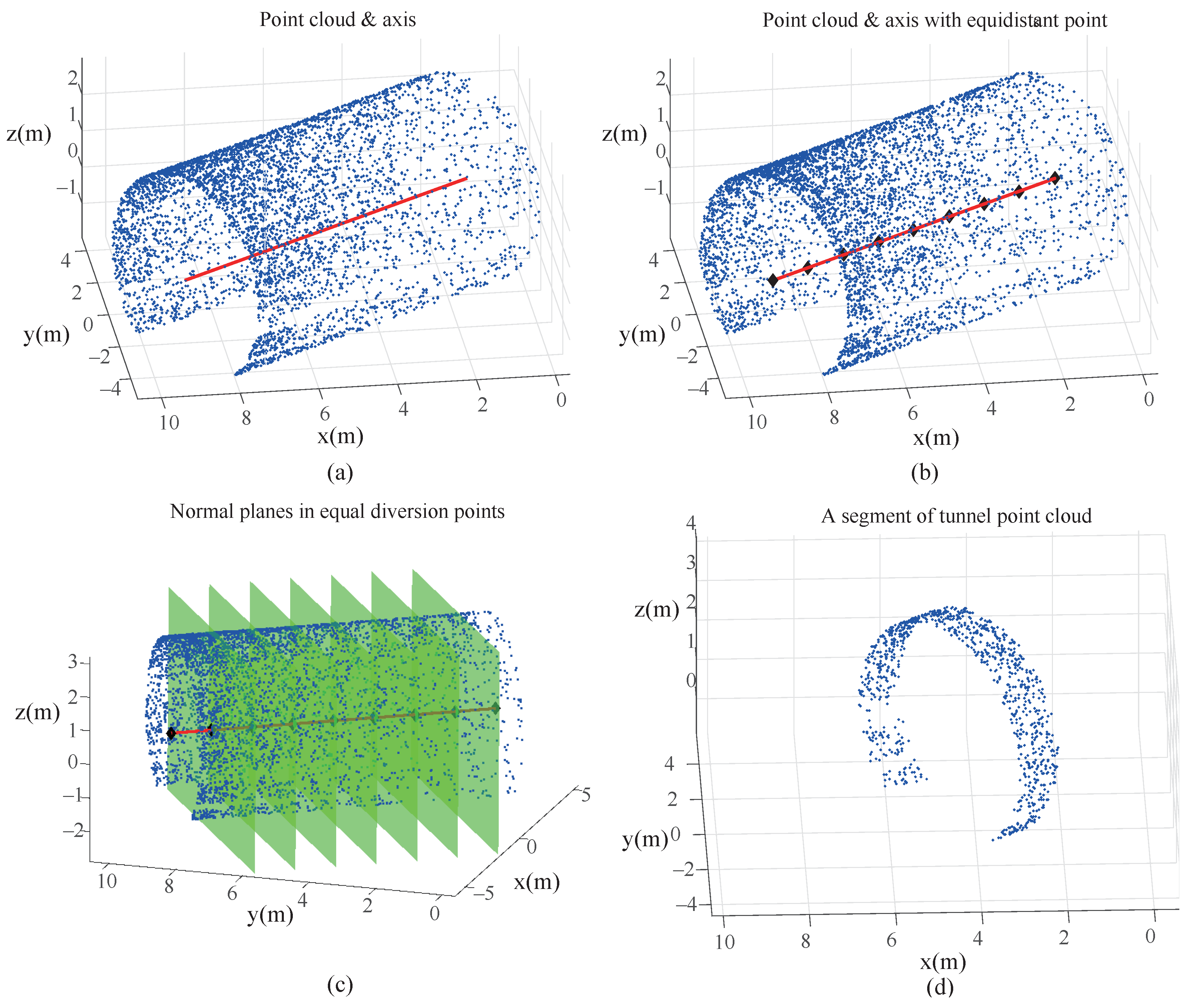
• Cut out a section of the tunnel point clouds with n linings and the axis acquired in Section 2.2;
• Divide the axis into n segments equally and get $n-1$ equal division points in the axis;
• Divide the selected tunnel point clouds by the normal planes of the axis with equal division points into n segments;
• Extract the tunnel point cloud segments between the two adjacent normal planes.

2.4. Point Cloud Data Denoising

Various errors and noise exist in the acquired data, and denoising is thus very essential. The raw tunnel point clouds contain two main kinds of noise: the first kind of noise is generated as a result of facilities and equipment in the tunnel; the second kind of noise is generated due to unusual reflectivity of the scanned surface, which generally occurs with light-reflecting and light-absorption surfaces. The first kind of noise is obvious and easy to locate. The second kind of noise has a negative effect on the result accuracy and is difficult to locate and distinguish because it is randomly distributed in point clouds. The second kind of noise can be eliminated in the processors based on the RANSAC algorithm. The denoising module based on clustering is mainly focused on the first kind of noise.

The proposed denoising algorithm employs the K-means algorithm to perform a cluster analysis based on the distance and intensity. Firstly, the structure point clouds are clustered based on the difference between the distances between the tunnel axis and the facilities in the tunnel and the distances between the tunnel axis and the surfaces of tunnel linings. However, some facilities are very close to the tunnel surface, and the connecting pieces are in direct contact with the tunnel lining so the difference in distance is too small to cluster. In conclusion, it is hard to eliminate the point clouds generated by the facilities efficiently and accurately. On the other hand, the LiDAR intensity is based on the optical strength which is highly dependent on the reflectance properties of the scanned materials [30]. Thus, different materials may reflect laser beams with different intensity strengths even when they have equal distances and incidence angles. The facilities and equipment in the tunnel are generally made of metal and rubber, or the surface is covered with paint, which is totally different from concrete tunnel lining surfaces with respect to the reflectance properties. The proposed algorithm employs the second clustering method based on the intensity of the outcome of clustering based on distance to assist the analysis and improve the accuracy. The flowchart of the proposed algorithm is illustrated in Figure 5.

The first clustering method is based on distance, and the following are the steps of the first clustering method:

• Implement the clustering analysis in every segment extracted, as described in Section 2.3, to reduce the complexity of the algorithm and improve the stability while assuring accuracy;
• Normalize the coordinates of the axis and tunnel point cloud segment. Transfer the tunnel point cloud segment using the coordinate transformation matrix to the point where the tunnel axis is coincident with the designed coordinate axis;
• Cluster the tunnel point clouds based on distance. Label points of classes as follows: $str$ stands for point clouds rejected by the structure and $equ$ represents point clouds from facilities and equipment once point clouds have been clustered. Calculate the distances between every single point in the point clouds and the tunnel axis and then set threshold values ($R+$$\mathsf{\Delta }$r and $R-$$\mathsf{\Delta }$r) corresponding to the $str$ and $equ$ classes, respectively, where R is the radius of the tunnel, and $\mathsf{\Delta }$r is the distance threshold.

Tunnel point clouds contain massive amounts of data and result in huge time consumption. $\omega$ is set as the dilution factor for uniform sampling of the data to reduce the computational time:

$$N_A=\omega ·N_i,$$

(5)

where $N_i$ is the number of points in segment i, and $\omega$ is the dilution factor defined by the amount of data and the algorithm efficiency requirement; $N_A$ is the actual number of points in the calculation.

The second clustering analysis is based on intensity and is implemented on the result of the first clustering analysis. Akca suggested that intensity values can supply decent additional information for identification [31].

The second clustering method uses the labeled points as training samples to set up pattern statistics. The following are the steps of the second clustering method:

• Obtain the original clustering center of the two classes $str$ and $equ$ from the result of the first clustering analysis:

  $$C_0\left[C\right]=\frac{{\displaystyle \sum _{j\in C}}{I}_j}{N_C},$$

  (6)

  where $C_0$ is the initial clustering center, $I_J$ is the intensity value, C represents class $str$ or class $equ$, and $N_c$ is the total number of class $str$ or $equ$ points;
• Calculate the distance between every residual point and the two initial clustering centers and cluster the points to the nearest class. Then, recalculate the clustering centers of the two classes:

  $$C_k\left[C\right]=\frac{{\displaystyle \sum _{j\in C}}{I}_j}{N_C},$$

  (7)

  where k is the number of iterations.
• The iterative calculation ends when the difference between a new clustering center and last clustering center is equal to or less than the threshold.

Through verification by experiments, the proposed denoising algorithm can remove the point clouds reflected by facilities and equipment efficiently and accurately.

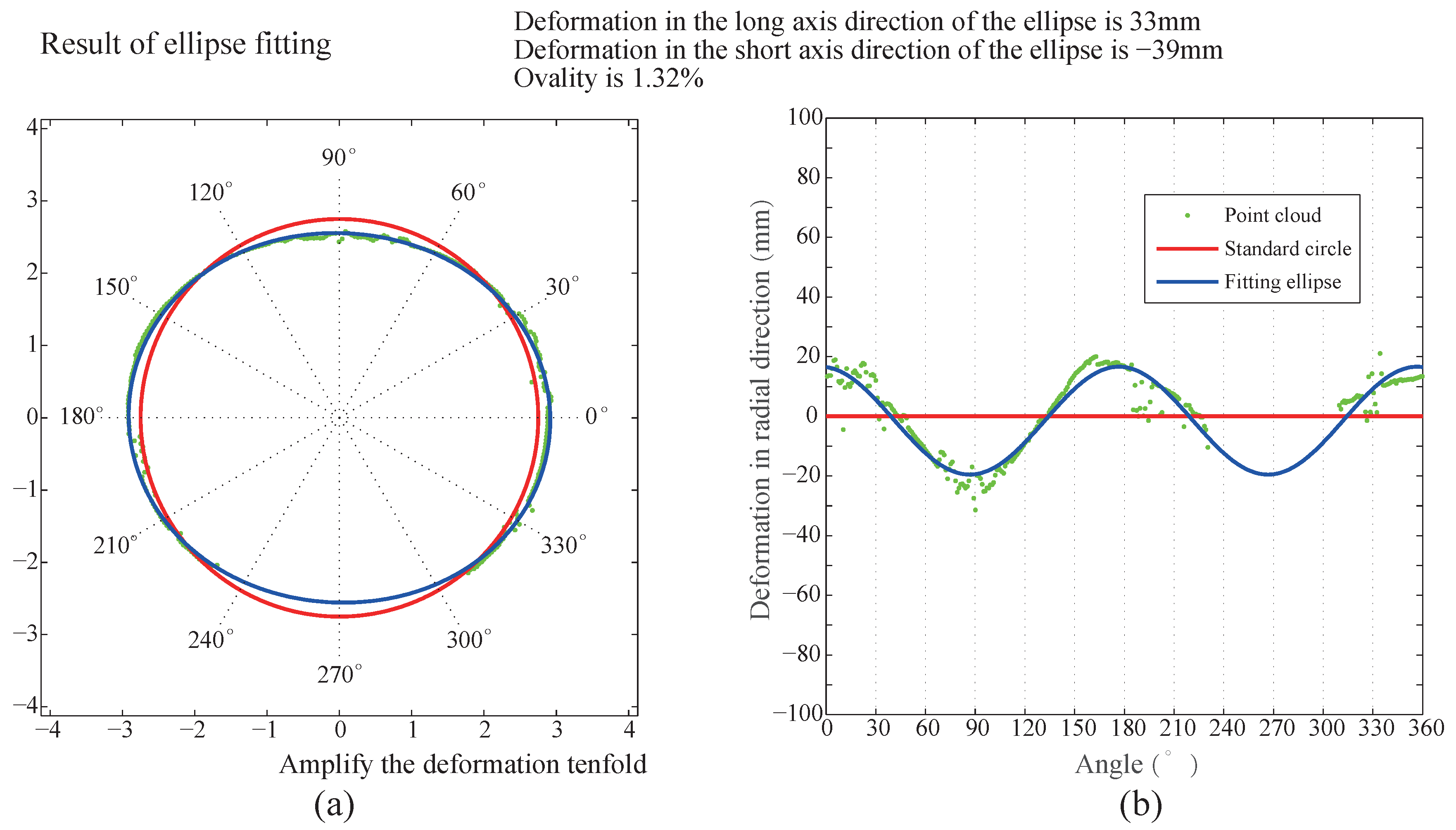
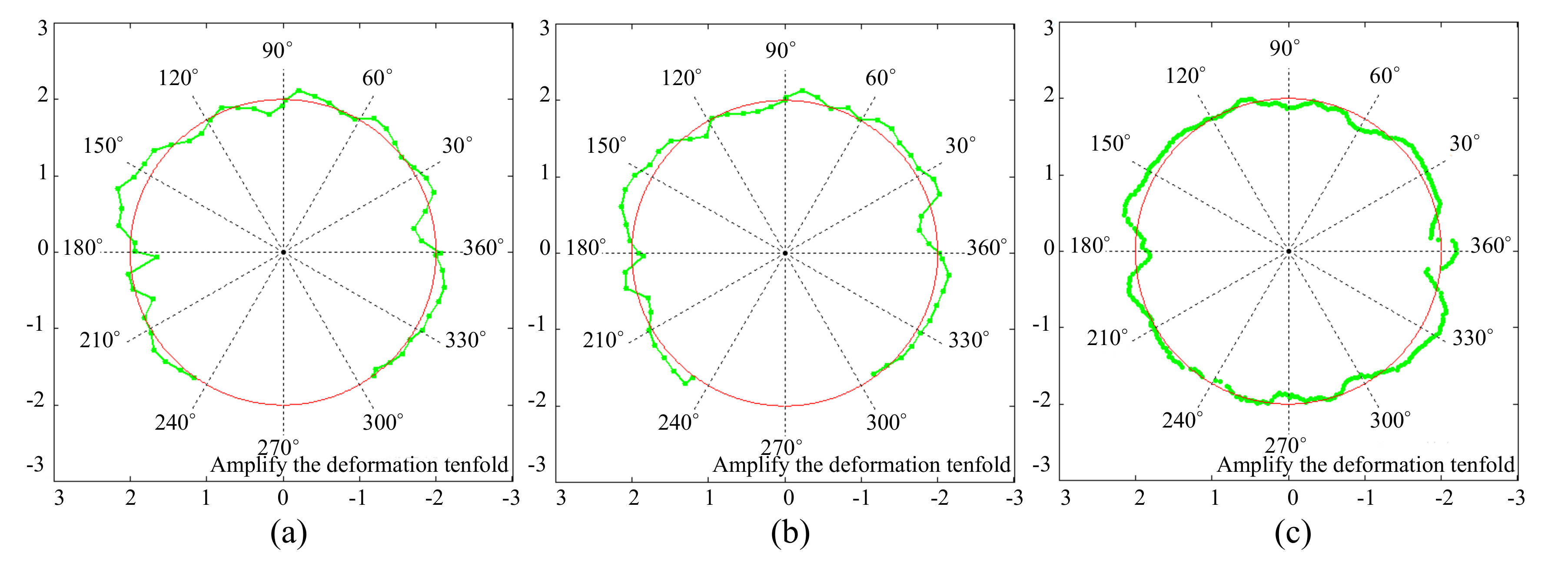
2.5. Extraction of Circular Tunnel Deformation

The proposed monitoring system can make full use of massive amounts of spatial data and deepen our cognition of the structure state greatly. This chapter digs deeper into the tunnel point cloud segments to obtain more comprehensive and visual information about the tunnel’s structural health.

According to the existing research and engineering experiences, tunnel deformation is one of the most direct indicators of a tunnel’s condition [32]. Thus, the proposed processing method uses radial deformation as the indicator to reflect the safety conditions of the tunnel structure.

In general, during operation, circular stormwater sewage tunnel structures become deformed before failure due to the nonuniform stress difference between surrounding strata and the inner water pressure. This stress distribution can be approximately treated as an ellipse with tiny differences between the long axis and the minor axis. Hereby, determination of the ovality and formation of the three-dimensional visualization deformation nephogram are employed to indicate the radial deformation of the tunnel structure [33].

The processor employs the RANSAC algorithm for curve-fitting to acquire the ellipse of the tunnel cross-section formed by scanned points. The ovality is illustrated by the following formula where T represents the tunnel ovality:

$$T=\frac{F-f}{D},$$

(8)

where F and f are the length of the major axis and the minor axis of the fitted ellipse, respectively; R is the design radial of the tunnel.

The three-dimensional visualization deformation nephogram based on regular point cloud gridding makes full use of the massive number of points collected by TLS and illustrates the deformation of a tunnel segment in a more detailed way.

The ovality and three-dimensional deformation nephogram can make full use of the massive amount of information contained in point clouds collected by TLS and demonstrate the deformation of almost every point in a tunnel, thereby reflecting its health condition.

3. Application

The proposed monitoring system aims to achieve automation and highly efficient LiDAR data processing for circular stormwater sewage tunnel structure health monitoring. This section describes the application of the proposed processing method and compares the efficiency of the automatic point cloud processing method with the conventional manual method.

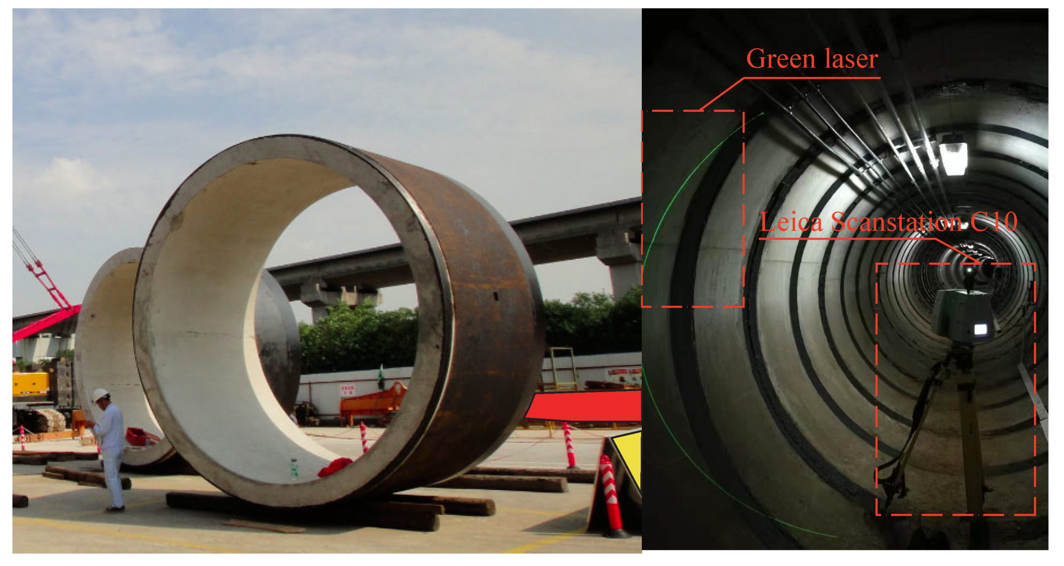
3.1. Practical Monitoring Project

To ensure the safe operation of Shanghai’s urban infrastructure, the circular sewage tunnel improvement project of the southern line of the Bailonggang area was initiated on 22 June 2010 with a total length of about 35 km and a designed sewage transportation capacity of about 2.2 million tons per day. The project services an area about 1255 square km and a population of about 7.12 million people.

LiDAR technology was applied to monitor the structure state of the circular sewage tunnel of the project during construction. The LiDAR data was scanned by Leica Scanstation C10 with medium resolution inside the tunnel along the axis, and the photograph of the tunnel lining and the device are shown in Figure 6.

The geometric arrangement of scan stations is indicated by Figure 7. $\mathsf{\Delta }$H (m) is defined as the vertical distance from the scan station to the center of the tunnel, and $\mathsf{\Delta }$T (m) is the horizontal distance.

In this application, the distance between two adjacent stations was chosen to be 12 m, and this included six tunnel lining segments, which were easy to locate, and a maximum incidence angle of ${62}^{\circ }$, which is less than the incidence angel limit of ${65}^{\circ }$. The whole monitoring zone was 150 m long and contained 75 tunnel lining segments. In total, there were 12 terrestrial laser scanning (TLS) scan stations and each two adjacent point clouds were assembled by three high definition surveying (HDS) targets between them.

In order to make the methodology clear, a sample of tunnel point clouds was extracted to demonstrate the whole process. Firstly, the steps of axis acquisition are denoted in Figure 8. Based on the projection of the compressed tunnel point cloud in the XOY plane, the upper and lower boundary points are extracted from every point cloud interval from $xmin$ to $xmax$. Then, the upper and lower boundaries are fitted through the boundary points by RANSAC and finally tunnel axis is extracted according to these two boundaries.

Based on the axis acquired in Figure 7, the tunnel point cloud was divided equally to extract point cloud segments, which was illustrated in Figure 8. Then, the tunnel axis and tunnel point cloud segments were processed and then applied to the denoising module.

The denoising module works with the results obtained from Figure 9, and the processes of the cluster analysis are shown in Figure 10 and Figure 11. In the first cluster, the distances of every single point in the raw point clouds and the probability distribution of the distances were illustrated in Figure 10a,b, respectively. It is obvious that most of the points are concentrated in the area around the distance of 2.75 m. The value of $\mathsf{\Delta }$r is taken to be greater than zero to ensure class $equ$ contains the points reflected by facilities and equipment only. However, class $str$ may also contain part of the equipment point clouds and is implemented twice in the clustering analysis based on intensity.

In the second cluster, the intensity distribution of retained point clouds after the first cluster and the probability distribution of the intensity were shown in Figure 11a,b, respectively. It is obvious that most of the points are concentrated in the area around $-1500$ to $-1000$.

Combining the results of two cluster analysis, Figure 12 illustrates the two-dimensional probability distribution of distance and intensity of the proposed algorithm.

After the tunnel point cloud data processing, the deformation of the circular stormwater sewage tunnel will be extracted from the clean point cloud segments without noise. Figure 13 denotes the ovality result of a tunnel point cloud segment produced by the proposed processing method, which provides quantificationally information of the tunnel deformation. Figure 14 denotes the three-dimensional deformation nephogram of a single tunnel point cloud segment, which provides visualization results of the tunnel deformation.

Combining the three-dimensional nephogram of every segment, the overall deformation nephogram of the tunnel is illustrated in Figure 15, which provides the visualization result of the entire tunnel.

3.2. Analysis of the Project Efficiency

The proposed method processes massive amounts of data in a fully automatic way, significantly improving the efficiency of point cloud processing and allowing the engineers to do other more meaningful work.

The steps of manual point cloud processing are as follows: first, label the tunnel linings in a fixed direction to increase the convenience of subsequent processing. Then, segment the tunnel point clouds and remove the obvious noise, namely, the points reflected by the facilities and equipment inside the tunnel. Next, implement ellipse-fitting for tunnel segment point clouds through business software to extract the axis. Finally, export the processed information. As for the stormwater sewage tunnel, based on past experience, the time consumed in processing a single tunnel lining point cloud segment is about six minutes.

The monitored zone contains 75 tunnel lining segments and the point cloud data scanned in the zone were processed by the conventional method and the proposed method separately, by the same computer.

Table 1. Comparison of post-processing time between the two methods.

The Proposed Monitoring System		Conventional Manual Way
Steps	Times/s	Steps	Times/s
Axis acquisition	30	Label linings	5000
Segment extraction	2.5	Segment extraction	6500
Denoising	17.5	Denoising	8000
		Axis extraction	10,000
		Error correction	5000

denotes the differences between the results of the two methods.

According to the comparison in the above table, the largest components of computational time consumed in the conventional method are manual noise removal, lining segment division, and tunnel axis extraction. These manual operations are not only time-consuming, but they also adversely affect the accuracy.

The conventional point cloud processing method mainly depends on manual operations and business software; it is a time-consuming and labor intensive process with low accuracy. The business software is designed for all customers from various industries, so most of the functions are universal and not specifically designed for circular tunnel point cloud processing. The manual extraction of tunnel lining segments cannot provide precise measurements due to the manual partitioning of tunnel point clouds which totally depends on determining the differences in joint intensity with the naked eye. The manual removal of obvious noise reflected by facilities inside the tunnel is very cursory because the selection tool in Cyclone is fixed, and it does not suit the geometry of tunnel point clouds. On the other hand, defects in the manual removal of noise also result in over-denoising or inadequate denoising.

According to the analysis above, the proposed monitoring system was successfully applied in practical engineering and completed the monitoring task automatically and efficiently.

4. Error Analysis

Errors of the proposed processing method mainly consist of single point location errors, measuring errors, and algorithm errors. Single point location errors are determined by the accuracy of the scanner hardware. The TLS point cloud data were acquired from the Leica Scanstation C10 and measurements taken with this type of laser scanner resulted in a range precision of 4 mm and a range distance of 134 m at a reflectivity of 90%. The measuring error can be efficiently restricted within the permissible range by adjusting the distance between two adjacent stations and the incidence angle. The algorithm error occurs as a result of some unavoidable limitations of the algorithm. It will transmit and amplify the deviation, and it is difficult to evaluate [34].

An operation was simulated to analyze the error produced in the proposed monitoring system. A conventional monitoring system based on the station as a whole was applied for comparison, and the surveying results were compared to quantify the error and obtain the realistic accuracy of the proposed processing method. The experiment was conducted in a pipe-jacking circular sewage tunnel lining with a 4 m diameter. Measurements of 55 points in the same cross-sectional area of the tunnel lining were made by the conventional monitoring system based on the station as a whole twice, and then the tunnel lining was scanned by TLS. The instrument parameters applied at the two monitoring systems are shown in

Table 2. The instrument parameters of the laser scanner and the station as a whole used in the two monitoring systems.

	Total Station	Laser Scanner
Name	Leica TS30	Leica C10
Angle accuracy	0.5${}^{″}$	12${}^{″}$
Range accuracy	2 mm + 2 ppm	4 mm (50 m)

. Figure 15 illustrates the tunnel lining profiles fitted by two sets of data collected by the station as a whole and by the point clouds scanned by TLS, respectively.

The measurement results from the station as a whole are treated as the reference due to their high precision in analyzing the accuracy of the proposed monitoring system. The differences between the distances of points with the same central angle measured by the station as a whole were calculated, and the TLS values of different measurements were used as the measurement error of the proposed monitoring system. The histograms were obtained (Figure 16).

The measurements illustrated in Figure 16 were input for statistical analysis with the Jarque–Bera test. The measurement error shown in the left of Figure 17 follows a normal distribution with a mean value of 0.1 mm and a standard deviation of 1.2 mm, and the measurement error shown on the right also follows a normal distribution with a mean value of $-0.1$ mm and a standard deviation of 1.2 mm.

5. Conclusions

This article proposed an automatic circular stormwater sewage tunnel point cloud processing method based on LiDAR data that measures the tunnel deformation by its ovality and a three-dimensional visualization nephogram.

The proposed processing method puts forward a series of efficient and robust algorithms to automatically process point clouds of the circular stormwater sewage tunnel. Firstly, it extracts the tunnel axis using algorithms based on RANSAC. Then, it extracts tunnel segments from the entire tunnel point clouds precisely by equally dividing the axis; next, it removes the obvious noise by two clustering methods. Finally, it obtains the ovality and tunnel deformation visualization nephogram to evaluate the circular stormwater sewage tunnel radial deformation. The indicators employed in the result analysis, especially the visualization nephogram, obtain more abundant reference information and can take full advantage of the massive amount of information from LiDAR data. However, the entire processing method is designed based on circular tunnels and can not be applied to irregular tunnels. Future research needs to focus on extending the applicable tunnel types of the method.

The proposed monitoring system mainly focuses on the automation of LiDAR data processing and the visualization of deformation. The aim is to apply LiDAR technology to circular stormwater sewage tunnel monitoring. The analysis of the field contrast test and the practical application in the Bailonggang sewage tunnel improvement project during construction suggested that the proposed processing method significantly improves the efficiency of point cloud processing with sufficient precision. Thus, LiDAR technology can be successfully applied to circular stormwater sewage tunnel monitoring.

References

1. Riveiro, B.; DeJong, M.J.; Conde, B. Automated processing of large point clouds for structural health monitoring of masonry arch bridges. Autom. Constr. 2016, 72, 258–268. [Google Scholar] [CrossRef]
2. Díaz-Vilariño, L.; González-Jorge, H.; Bueno, M. Automatic classification of urban pavements using mobile LiDAR data and roughness descriptors. Constr. Build. Mater. 2016, 102, 208–215. [Google Scholar] [CrossRef]
3. Vazaios, I.; Vlachopoulos, N.; Diederichs, M.S. Integration of Lidar-based structural input and discrete fracture network generation for underground applications. Geotech. Geol. Eng. 2017, 35, 2227–2251. [Google Scholar] [CrossRef]
4. Palmer, D.; Koumpli, E.; Cole, I. A GIS-Based Method for Identification of Wide Area Rooftop Suitability for Minimum Size PV Systems Using LiDAR Data and Photogrammetry. Energies 2018, 12, 3506. [Google Scholar] [CrossRef]
5. Le Clainche, S.; Lorente, L.; Vega, J.; Vega Jose, M. Wind Predictions Upstream Wind Turbines from a LiDAR Database. Energies 2018, 3, 543. [Google Scholar] [CrossRef]
6. Yan, Y.; Tan, Z.; Su, N. Building Extraction Based on an Optimized Stacked Sparse Autoencoder of Structure and Training Samples Using LIDAR DSM and Optical Images. Sensors 2017, 17, 1957. [Google Scholar] [CrossRef] [PubMed]
7. Bosché, F.; Ahmed, M.; Turkan, Y. The value of integrating Scan-to-BIM and Scan-vs-BIM techniques for construction monitoring using laser scanning and BIM: The case of cylindrical MEP components. Autom. Constr. 2015, 49, 201–213. [Google Scholar] [CrossRef]
8. Argüelles-Fraga, R.; Ordóñez, C.; García-Cortés, S. Measurement planning for circular cross-section tunnels using terrestrial laser scanning. Autom. Constr. 2013, 31, 1–9. [Google Scholar] [CrossRef]
9. Roca-Pardiñas, J.; Argüelles-Fraga, R.; de Asís López, F. Analysis of the influence of range and angle of incidence of terrestrial laser scanning measurements on tunnel inspection. Tunn. Undergr. Space Technol. 2014, 43, 133–139. [Google Scholar] [CrossRef]
10. Pejić, M. Design and optimisation of laser scanning for tunnels geometry inspection. Tunn. Undergr. Space Technol. 2013, 37, 199–206. [Google Scholar] [CrossRef]
11. Guo, J.; Tsai, M.J.; Han, J.Y. Automatic reconstruction of road surface features by using terrestrial mobile lidar. Autom. Constr. 2015, 58, 165–175. [Google Scholar] [CrossRef]
12. Cabo, C.; Cortés, S.G.; Ordoñez, C. Mobile Laser Scanner data for automatic surface detection based on line arrangement. Autom. Constr. 2015, 58, 28–37. [Google Scholar] [CrossRef]
13. Kim, J.U.; Kang, H.B. A new 3D object pose detection method using LIDAR shape set. Sensors 2018, 18, 882. [Google Scholar] [CrossRef] [PubMed]
14. Puente, I.; González-Jorge, H.; Martínez-Sánchez, J. Automatic detection of road tunnel luminaires using a mobile LiDAR system. Measurement 2014, 47, 569–575. [Google Scholar] [CrossRef]
15. Kashani, A.G.; Graettinger, A.J. Cluster-Based Roof Covering Damage Detection in Ground-Based Lidar Data. Autom. Constr. 2015, 58, 19–27. [Google Scholar] [CrossRef]
16. Kashani, A.G.; Olsen, M.J.; Graettinger, A.J. Laser Scanning Intensity Analysis for Automated Building Wind Damage Detection. Cong. Comput. Civ. Eng. Proc. 2015, 199–205. [Google Scholar] [CrossRef]
17. Nuttens, T.; Stal, C.; De Backer, H. Methodology for the ovalization monitoring of newly built circular train tunnels based on laser scanning: Liefkenshoek Rail Link (Belgium). Autom. Constr. 2014, 43, 1–9. [Google Scholar] [CrossRef]
18. Han, J.Y.; Guo, J.; Jiang, Y.S. Monitoring tunnel profile by means of multi-epoch dispersed 3-D LiDAR point clouds. Tunn. Undergr. Space Technol. 2013, 33, 186–192. [Google Scholar] [CrossRef]
19. Han, J.Y.; Guo, J.; Jiang, Y.S. Monitoring tunnel deformations by means of multi-epoch dispersed 3D LiDAR point clouds: An improved approach. Tunn. Undergr. Space Technol. 2013, 38, 385–389. [Google Scholar] [CrossRef]
20. Janowski, A. The circle object detection with the use of Msplit estimation. EDP Sci. 2018, 26, 00014. [Google Scholar] [CrossRef] [Green Version]
21. Janowski, A.; Bobkowska, K.; Szulwic, J. 3D modelling of cylindrical-shaped objects from lidar data-an assessment based on theoretical modelling and experimental data. Metrol. Meas. Syst. 2018, 25, 47–56. [Google Scholar] [CrossRef]
22. Arastounia, M. Automated as-built model generation of subway tunnels from mobile LiDAR data. Sensors 2016, 16, 1486. [Google Scholar] [CrossRef] [PubMed]
23. Puente, I.; Akinci, B.; González-Jorge, H. A semi-automated method for extracting vertical clearance and cross sections in tunnels using mobile LiDAR data. Tunn. Undergr. Space Technol. 2016, 59, 48–54. [Google Scholar] [CrossRef]
24. Ge, Y.; Tang, H.; Xia, D. Automated measurements of discontinuity geometric properties from a 3D-point cloud based on a modified region growing algorithm. Eng. Geol. 2018, 242, 44–54. [Google Scholar] [CrossRef]
25. Chen, S.; Walske, M.L.; Davies, I.J. Rapid mapping and analysing rock mass discontinuities with 3D terrestrial laser scanning in the underground excavation. Int. J. Rock Mech. Min. Sci. 2018, 110, 28–35. [Google Scholar] [CrossRef]
26. Sánchez-Rodríguez, A.; Riveiro, B.; Soilán, M. Automated detection and decomposition of railway tunnels from Mobile Laser Scanning Datasets. Autom. Constr. 2018, 96, 171–179. [Google Scholar] [CrossRef]
27. Fumarola, M.; Poelman, R. Generating virtual environments of real world facilities: Discussing four different approaches. Autom. Constr. 2011, 20, 263–269. [Google Scholar] [CrossRef]
28. Fischler, M.A.; Bolles, R.C. Random sample consensus: A paradigm for model fitting with applications to image analysis and automated cartography. Commun. ACM 1981, 24, 381–395. [Google Scholar] [CrossRef]
29. Maalek, R.; Lichti, D.; Ruwanpura, J. Robust Segmentation of Planar and Linear Features of Terrestrial Laser Scanner Point Clouds Acquired from Construction Sites. Sensors 2018, 18, 819. [Google Scholar] [CrossRef]
30. Pfeifer, N.; Dorninger, P.; Haring, A. Investigating terrestrial laser scanning intensity data: Quality and functional relations. In Proceedings of the 8th Conference on Optical 3-D Measurement Techniques, Zurich, Switzerland, 9–12 July 2007; pp. 328–337. [Google Scholar]
31. Akca, D. Matching of 3D surfaces and their intensities. ISPRS J. Photogramm. Remote Sens. 2007, 62, 112–121. [Google Scholar] [CrossRef] [Green Version]
32. Qingwu, H.; Wanling, Y. Tempo-space Deformation Detection of Subway Tunnel based on Sequence Temporal 3D Point Cloud. Disaster Adv. 2012, 5, 1326–1330. [Google Scholar]
33. Li, X.; Yang, B.; Xie, X. Influence of Waveform Characteristics on LiDAR Ranging Accuracy and Precision. Sensors 2018, 18, 1156. [Google Scholar] [CrossRef]
34. Gao, Z.; Lao, M.; Sang, Y. Fast Sparse Coding for Range Data Denoising with Sparse Ridges Constraint. Sensors 2018, 18, 1449. [Google Scholar] [CrossRef] [PubMed]
Figure 1. Flow chart of the proposed monitoring system.
Energies 12 01599 g001
Figure 2. Flow chart of the acquisition of the circular tunnel axis.
Energies 12 01599 g002
Figure 3. The intuitive figure of the acquisition of the circular tunnel axis.
Energies 12 01599 g003
Figure 4. Flow chart of the tunnel point cloud segment extraction.
Energies 12 01599 g004
Figure 5. Flow chart of the proposed denoising algorithm using double clustering based on the distance and intensity.
Energies 12 01599 g005
Figure 6. The pipe-jacking circular sewage tunnel lining and Leica Scanstation C10 in the tunnel.
Energies 12 01599 g006
Figure 7. The geometric arrangement of the scan station of terrestrial laser scanning (TLS) in circular tunnels: the left picture illustrates the cross section which contains points A and B in the right picture; the right picture is the longitudinal section of tunnel and contains points A and B in the left picture.
Energies 12 01599 g007
Figure 8. The sketch of every single step in tunnel axis acquisition: (a) is the projection of the compressed tunnel point cloud in the XOY plane; (b) illustrates the upper points extracted from every point cloud interval from x m i n to x m a x ; (c) illustrates the lower boundary points extracted from every point cloud interval from x m i n to x m a x ; (d) illustrates the point cloud projection and all boundaries including inline and outline upper boundaries and inline and outline lower boundaries fitted through the points extracted in (b,c) by Random Sample Consensus (RANSAC); (e) illustrates all boundaries fitted through the boundary points by RANSAC; (f) extract the inline upper and lower boundaries and the axis extracted from the inline boundaries.
Energies 12 01599 g008
Figure 9. The procedure of tunnel point cloud segment extraction: (a) illustrates the tunnel point clouds with the axis; (b) illustrates the equal division in the axis of a section of a tunnel point cloud; (c) illustrates that the normal planes with equal division points divide the tunnel point clouds into lining segments; (d) illustrates the tunnel point cloud segment used for subsequent data processing.
Energies 12 01599 g009
Figure 10. Distance distribution of raw point clouds in experiments: (a) illustrates the three-dimensional spatial distribution of the tunnel point cloud about distance; (b) illustrates the quantity distribution of the tunnel point cloud about distance.
Energies 12 01599 g010
Figure 11. Intensity distribution of the raw point clouds in the experiments: (a) illustrates the three-dimensional spatial distribution of the tunnel point cloud about intensity; (b) illustrates the quantity distribution of the tunnel point cloud about intensity.
Energies 12 01599 g011
Figure 12. Two-dimensional probability distribution of distances and intensities.
Energies 12 01599 g012
Figure 13. The ovality of a tunnel point cloud segment produced by the proposed monitoring system: (a) is the comparison between the ellipse fitted by the point cloud and the standard circle which represents the designed schema; (b) is the unfolding drawing of (a) and illustrates a more intuitive comparison of the deformation from different central angles.
Energies 12 01599 g013
Figure 14. The three-dimensional deformation nephogram of a single tunnel point cloud segment. The different values of deformation are expressed by different colors.
Energies 12 01599 g014
Figure 15. The overall deformation nephogram of Shanghai metro line 7.
Energies 12 01599 g015
Figure 16. The profiles fitted by the data acquired in the experiments: (a) denotes the profile fitted by the first set of data collected by the station as a whole; (b) denotes the profile fitted by the second set of data collected by the station as a whole; (c) illustrates the profile fitted by the point cloud scanned by the TLS.
Energies 12 01599 g016
Figure 17. Histograms of differences between measurements by TLS and two measurements of the station as a whole: (a) denotes the quantitative distribution of the measurement error of the proposed monitoring system, which uses the first set of data from the station as the reference; (b) denotes the quantitative distribution of the measurement error of the proposed monitoring system, which uses the second set of data from the station as the reference.
Energies 12 01599 g017