Article

Cost-Benefit Analysis of Hybrid Photovoltaic/Thermal Collectors in a Nearly Zero-Energy Building
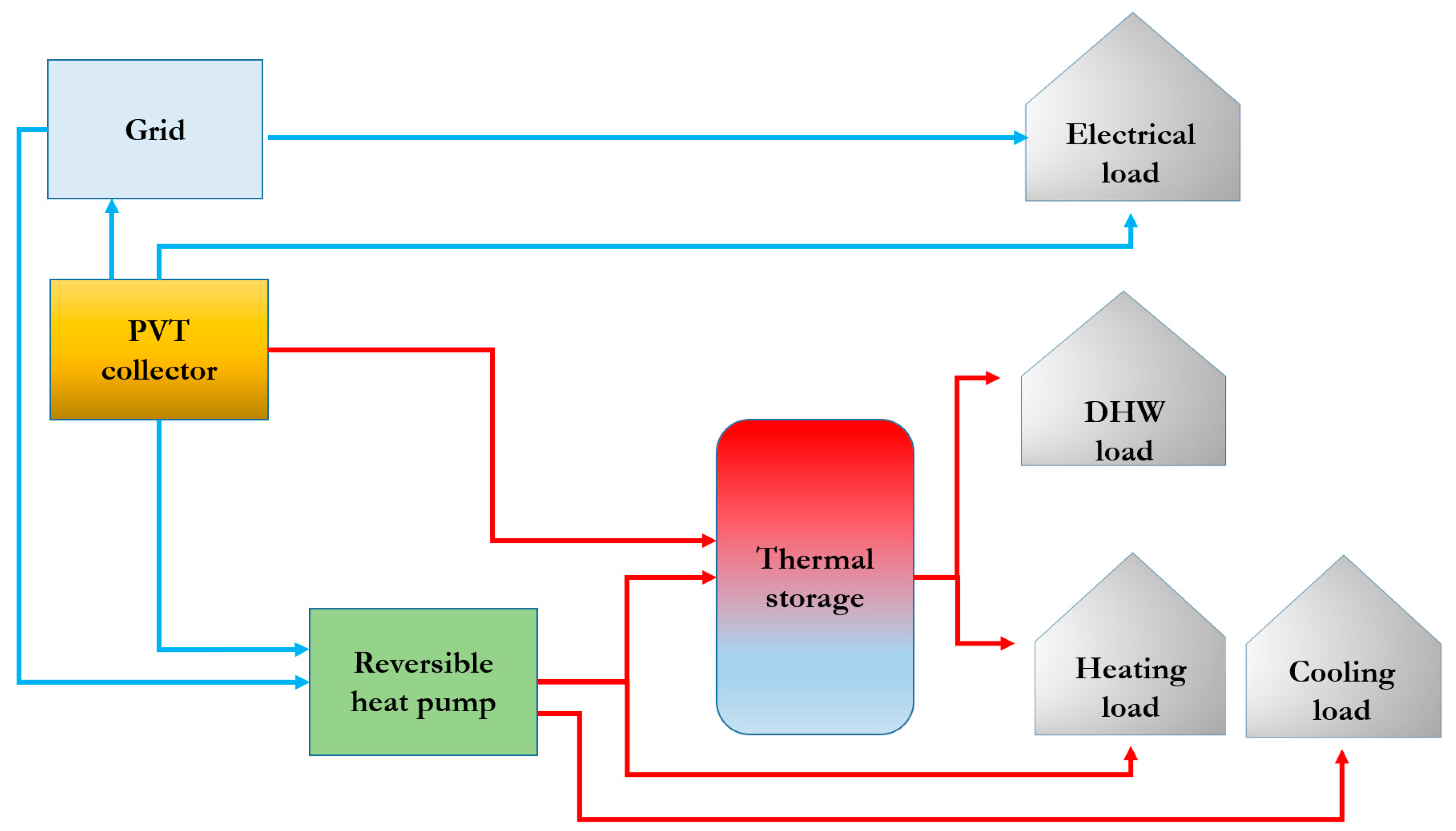
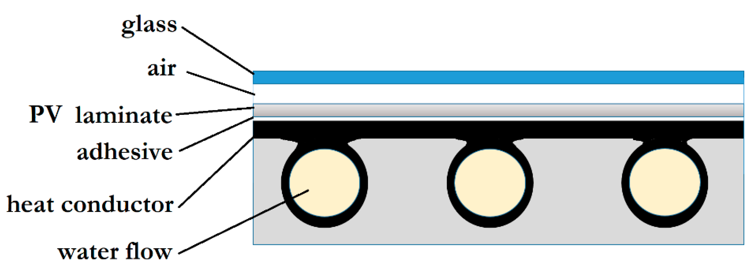
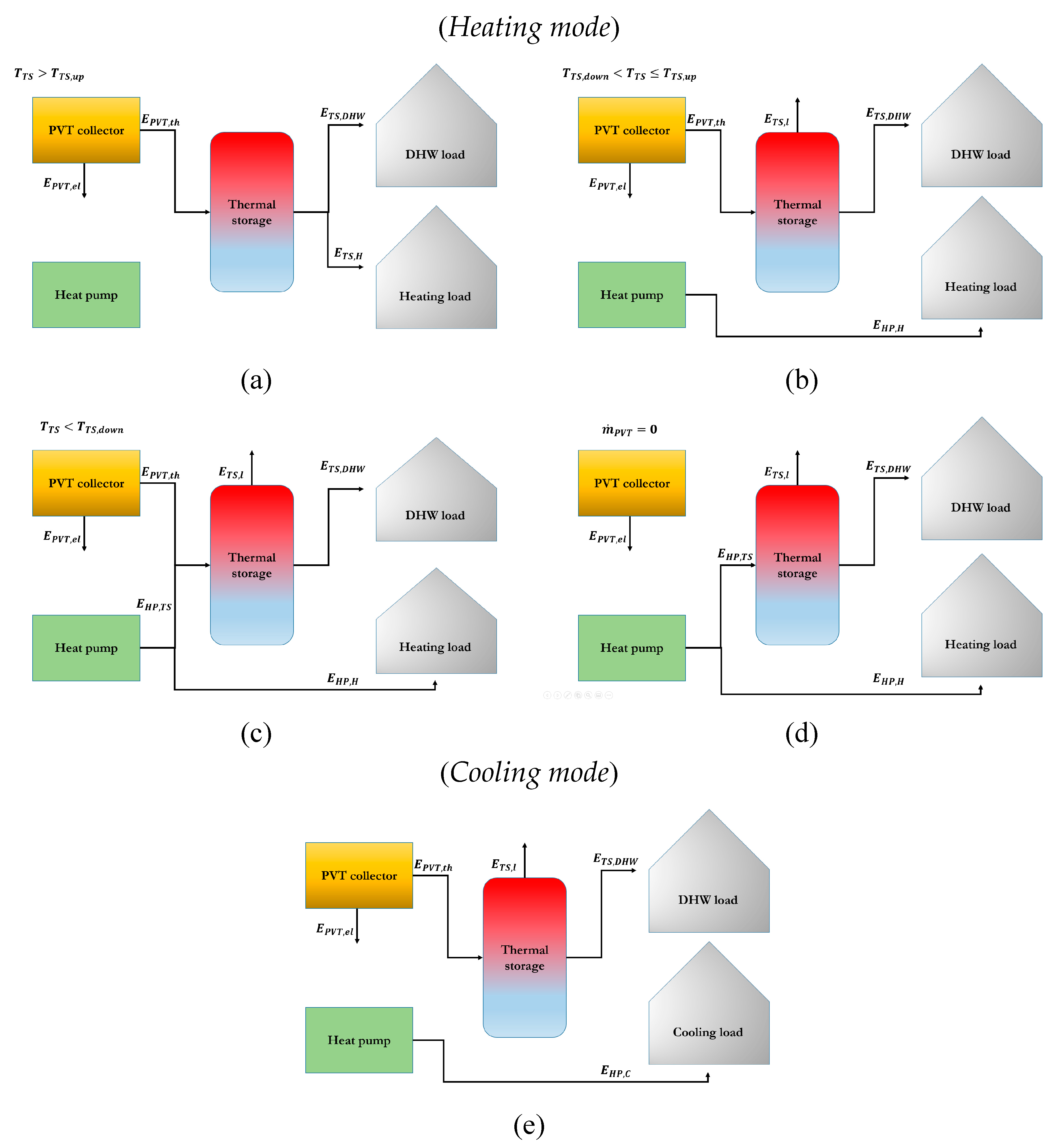
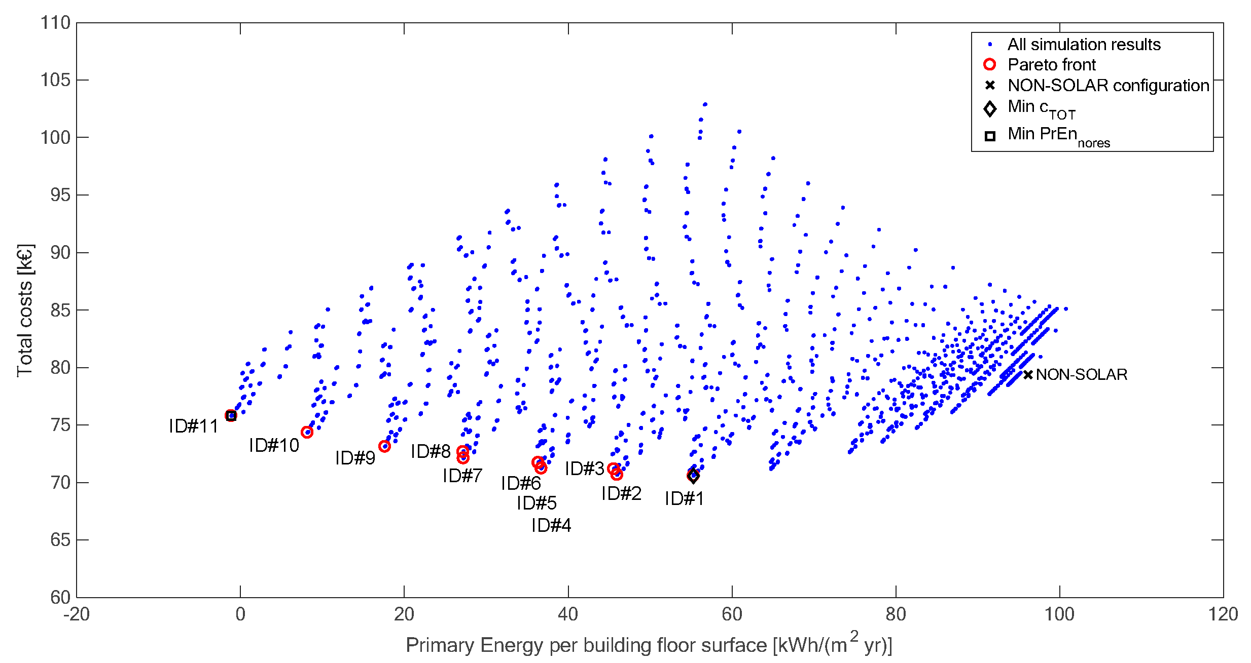
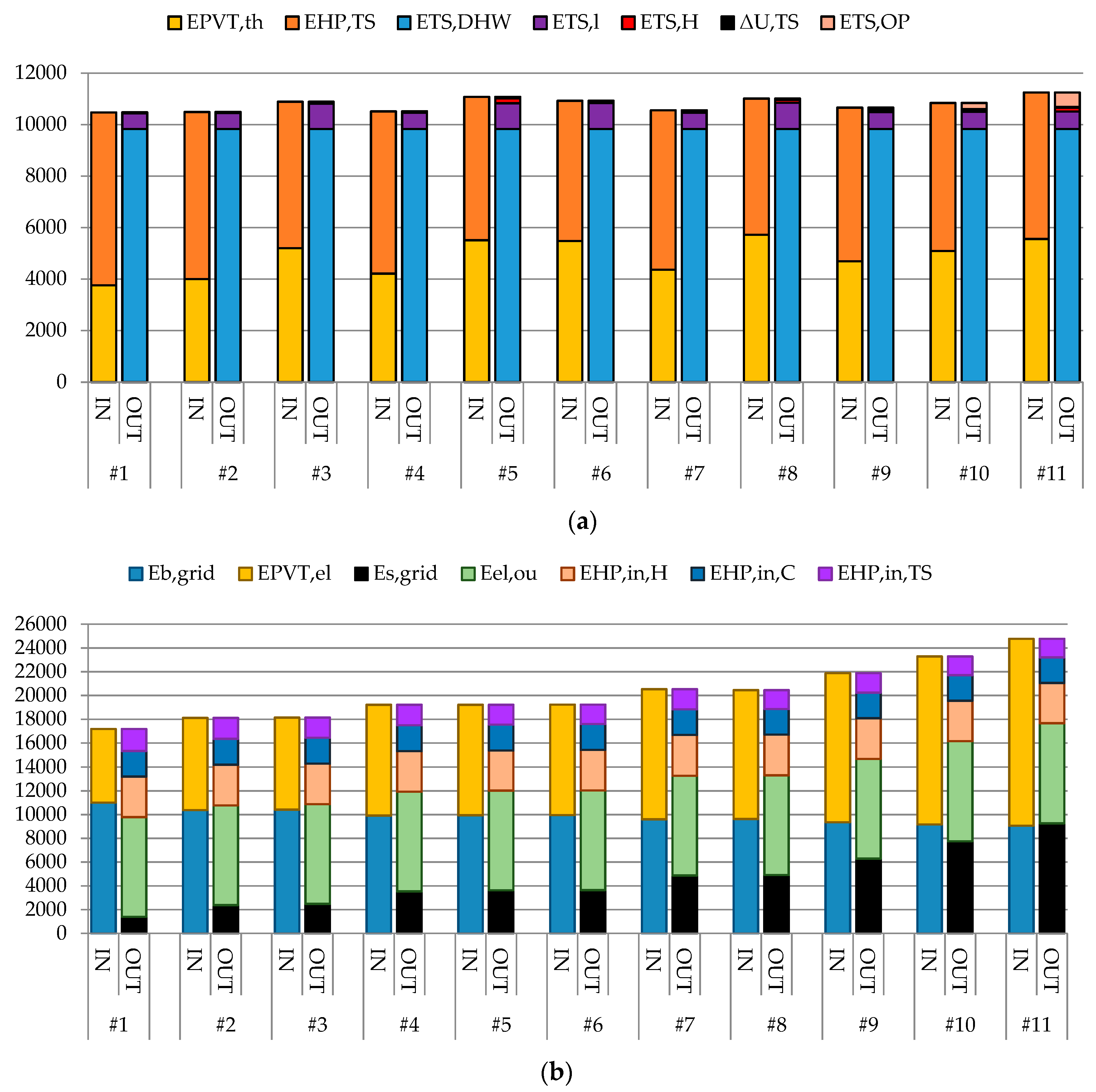
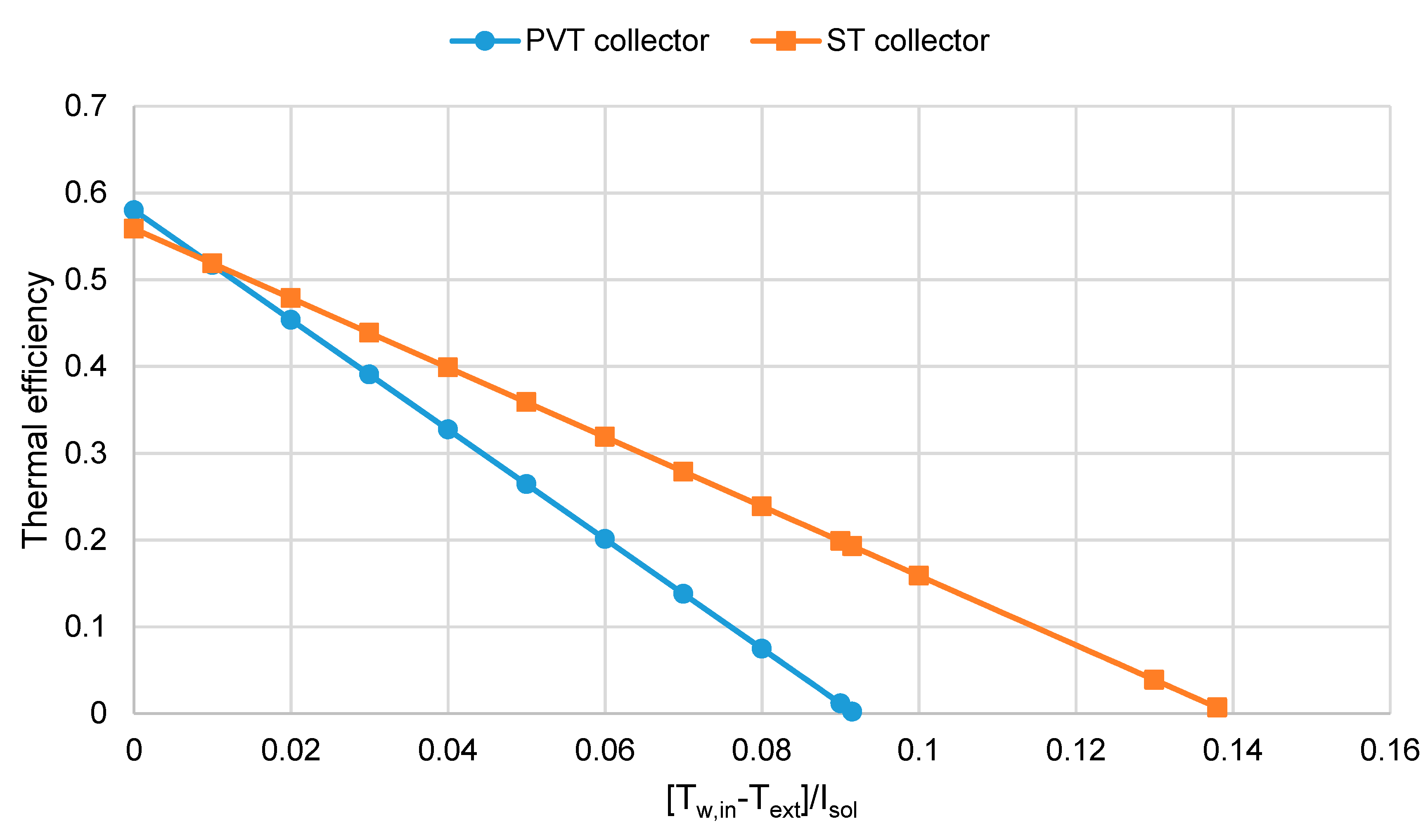
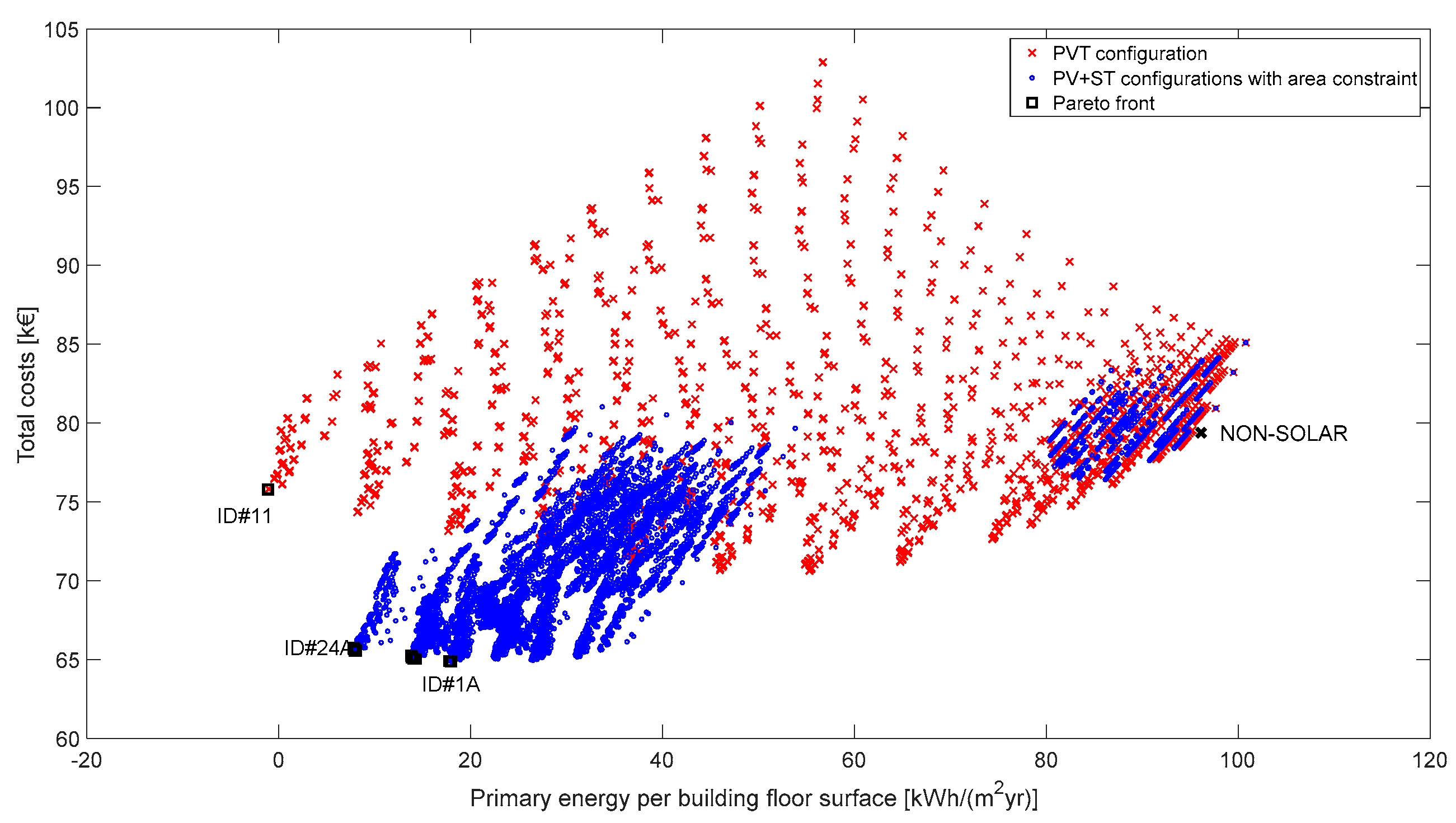
Building Energy Technique and Technology Research Group (BETTER), Department of Energy, Systems, Territory and Construction Engineering (DESTEC), University of Pisa, Largo Lucio Lazzarino, 56122 Pisa, Italy
*
Author to whom correspondence should be addressed.
Energies 2019, 12(8), 1582; https://doi.org/10.3390/en12081582
Submission received: 22 March 2019 / Revised: 19 April 2019 / Accepted: 21 April 2019 / Published: 25 April 2019

Abstract

:
This paper analyzes the use of hybrid photovoltaic/thermal (PVT) collectors in nearly zero-energy buildings (NZEBs). We present a design methodology based on the dynamic simulation of the whole energy system, which includes the building energy demand, a reversible heat pump as generator, the thermal storage, the power exchange with the grid, and both thermal and electrical energy production by solar collectors. An exhaustive search of the best equipment sizing and design is performed to minimize both the total costs and the non-renewable primary energy consumption over the system lifetime. The results show that photovoltaic/thermal technology reduces the non-renewable primary energy consumption below the nearly zero-energy threshold value, assumed as 15 kWh/(m2·yr), also reducing the total costs with respect to a non-solar solution (up to 8%). As expected, several possible optimal designs exist, with an opposite trend between energy savings and total costs. In all these optimal configurations, we figure out that photovoltaic/thermal technology favors the production of electrical energy with respect to the thermal one, which mainly occurs during the summer to meet the domestic hot water requirements and lower the temperature of the collectors. Finally, we show that, for a given solar area, photovoltaic/thermal technology leads to a higher reduction of the non-renewable primary energy and to a higher production of solar thermal energy with respect to a traditional separate production employing photovoltaic (PV) modules and solar thermal (ST) collectors.

1. Introduction

In the last decades, new solutions are studied to reduce energy requirements in the building sector, even with the aim to reach the nearly zero-energy level. In particular, the generation system including renewable energy sources, such as solar thermal panels and photovoltaic modules, are often analyzed [1,2,3,4,5]. The point of strength of these systems, in fact, is the possibility of being coupled with thermal storages, low-temperature terminal units, and heat pumps, to address the energy requirements of the building in an efficient way. However, it is necessary to seek the optimal sizing and control strategy of the solar technologies to maximize the energy savings. Several studies have been published on this topic [6,7,8], finding that the possible savings depend on the characteristics of the buildings, the profiles of energy requirements, and the characteristics of the overall system [9].
Among the classical solutions using separate modules, more attention is now given to hybrid photovoltaic/thermal collectors, also named PVT collectors. These collectors are a promising technology, combining in a single component both photovoltaic modules and solar collectors. Their main advantages are the reliability, the low maintenance, and the clean technology [10]; however, as they are still an emerging technology, their application in practical cases needs further study [11]. The PVT collector can be classified depending on the coolant fluid used, which is usually air or water. Several configurations are presented in literature, depending on the position of the absorber and the photovoltaic layer (see [10,11] for a complete analysis of the various possible configurations). Innovative designs are also present in literature: for example, in [12], the authors test a new PVT collector where water is directly in contact with the photovoltaic (PV) panel, without serpentines, showing good performances, even if the thermal efficiency is found to be strongly dependent on the flow rate. In [13], the authors propose instead a PVT collector where the water flows over the PV layer: the water flow absorbs infrared radiation, without modifying the visible spectrum, which instead is responsible for a good PV efficiency. Experimental results of this collector show that this PVT panel performs better than traditional ones in the case of large values of solar irradiance, due to the reduction of losses. In the last years, scientific literature reports several case studies of application of PVT collectors in building applications. For example, in [14], the authors study the feasibility of a system including a PVT collector, a thermal wheel, and an air-handling unit, finding that this solution allows a good energetic performance and a reduction of the energy requirements for the exhaust air heat recovery. In [15], the authors present the case study of a PVT collector connected to a thermal storage. The aim of the study is the identification of the optimal control of the water flow rate to maintain a high electrical efficiency and, at the same time, meet the domestic hot water (DHW) energy demand of the building. Two profiles of optimal control are found, one for winter and one for summer, which lead to significant energy and economic savings with respect to the suboptimal solution. In [16], the authors compare several solutions using water heat pumps as main generators, and photovoltaic modules, flat plane collectors or PVT collectors as renewable energy sources that provide useful energy for the generator and for the building requirements. Results show that the use of PVT collectors is associated with the lowest electrical energy requirements from the grid, also in different scenarios of electricity prices.
The use of PVT collectors in nearly zero-energy buildings (NZEBs) is not widespread in literature, since the analysis is often focused only on the solar collector and its energy conversion efficiency. However, this topic is important, considering the current targets in reducing the building energy requirements, especially for new and renovated ones. In this paper, the application of PVT collectors in NZEBs is investigated through a cost-benefit analysis of a case study constituted by a farm hostel served by a reversible heat pump, PVT collectors, and a thermal storage, for the heating, cooling, domestic hot water, and electrical energy services. We verify the achievement of the NZEB target assumed as a building with net primary energy consumption lower than 15 kWh/(m2·yr) [17].
The optimal design and control will be found through an exhaustive-enumeration multi-objective optimization in a dynamic simulation of the overall system, using as optimization variables the number, the azimuth, and the slope of PVT collectors, together with the volume and the control temperature of the thermal storage. The objective functions are the non-renewable primary energy and the total costs (sum of installation costs and operational costs), both evaluated at the end of the system lifetime. A set of possible design alternatives on the Pareto frontier is provided to the decision makers. Furthermore, the optimal solutions will be compared with the results of a similar optimization in a case study where the PVT collectors are substituted by traditional photovoltaic (PV) modules and solar thermal (ST) collectors. In this way, possible advantages and disadvantages of the PVT collectors can be highlighted with respect to traditional solutions.
Section 2 presents the description and modeling of the case study, including the heat pump, thermal storage, PVT collectors, and the control system. Section 3 presents the optimization problem and the analysis of the results. Section 4 presents the description of the case study with the PV and ST collectors separately and the results of the comparison of the optimization problem referred to the PVT case and the PV/ST case, from an energetic and economic point of view. Section 5 illustrates the conclusions and future works.

2. Description and Modeling of the Case Study

The chosen case study is a farm hostel in Enna, Italy. The town has a favorable solar irradiance, which is expected to result in a significant energy contribution from solar generators (PV, ST, and PVT). Besides, the energy system includes an electrically driven air-to-water heat pump, a thermal storage, with the possibility of exchanging power with the electrical grid (see Figure 1). Both buildings and heating, ventilation, and air-conditioning (HVAC) equipment performances are simulated over a standard year of operation through established dynamic models and an hourly time step.
The Italian Thermotechnical Committee (CTI) provides the hourly values of the typical meteorological year (TMY), in terms of temperature, relative humidity, global solar irradiance on the horizontal plane, and wind speed [18]. Monthly averaged climate data are reported in Table 1.

2.1. Energy Requirements of the Building

The hourly energy demands of the building are related to the heating and cooling service, domestic hot water (DHW) production, and electrical energy for lighting and other uses. The heating and cooling loads are evaluated as a function of the envelope characteristics (e.g., geometry, materials thermo-physical properties), external climate and internal set point. The main characteristics of the building envelope are reported in Appendix A.
The hourly heating and cooling loads of the building have been evaluated through the methodology reported in [19], using the following equations:
E t h , H = P H ( 1 T e x t ¯ T d e s , H T o f f , H T d e s , H ) η H ( E e l , o u )
E t h , C = P C ( 1 T e x t * ¯ T d e s , C * T o f f , C T d e s , C * ) + η C ( E e l , o u )
T e x t ¯ ( t ) = 1 ϕ ¯ i = 0 ϕ ¯ T e x t ( t ϕ ¯ + i )
ϕ ¯ = i ( U A ) i ϕ i [ i ( U A ) i + H v e ]
T e x t * ( t ) = T e x t ( t ) + α S h e I s o l ( t )
where E t h , H and E t h , C are the hourly heating and cooling loads, respectively; P H and P C are the heating and cooling peak loads; T d e s , H is the design external temperature (−3 °C) for heating; T d e s , C * is the design sol-air external temperature (47 °C) for cooling. T e x t * is the sol-air temperature, used in summer to take into account the effects of solar irradiation together with the external temperature: the sol-air temperature is evaluated as in Equation (1e), in accordance with [20]. T o f f , H and T o f f , C are the external and sol-air temperatures at which thermal losses and gains balance, nullifying heating and cooling demands, respectively. T e x t ¯ is an effective external temperature based on the effective time shift of the building, ϕ ¯ , evaluated through Equation (1d) [21]. The gains due to the electrical residential equipment, E e l , o u , are considered as an additional cooling load or reduction of heating requirement, using the heat gain utilization factors, η C and η H , evaluated as in EN 52016 [22]. The adopted building model represents a good trade-off between simplified models (e.g., the energy signature method [23]) and dynamic models (e.g., TRNSYS). The former ones do not require a detailed knowledge of the building, simply employing a correlation between the external temperature and energy requirements, but results can be inaccurate; the latter ones, instead, need a significant number of inputs to provide accurate results. Moreover, they are often time-consuming, being less suitable for simulations and optimization of many interconnected components.
For the present case study, peak loads are equal to 15 kW for both heating and cooling. A typical users’ profile has been chosen, with peaks in weekends and summer [24]. This profile influences the internal loads and the energy requirements for DHW and electrical energy. The corresponding energy demand for DHW is evaluated through the following equation:
E t h , D H W = ρ W c W V D H W ( T D H W T a q u )
where T D H W is equal to 40 °C and T a q u is equal to 16 °C. Hourly schedules of electrical energy have been also evaluated, using typical demands and profiles of hostels with rooms (where typical household appliances are used, such as personal computers, TVs, chargers) and kitchens (where fridges and induction cooking are used). More details about the building and profiles can be found in [25] and in Appendix A.

2.2. Modeling of the System

The analyzed HVAC system consists of a reversible heat pump, a thermal storage, and PVT collectors. The thermal storage is the main thermal node of the system, as it provides energy to DHW and the heating loads and is heated by the PVT collectors and by the heat pump when the solar contribution is not enough to maintain the required temperature. The latter generator also meets the cooling demand and directly heats the building, according to the control strategy discussed in detail in Section 2.2.4. As for the electrical load, the grid delivers or receives the power surplus or deficit between the PVT production and electricity demand (heat pump included). Figure 1 represents a scheme of the overall system.

2.2.1. Modeling of the Heat Pump

The heat pump is a reversible air-to-water electrically driven one, with inverter: thus, the actual thermal output can be provided by the heat pump without a significant penalization of the coefficient of performance (COP). For the evaluation of the heat pump performance, the second-law efficiency method is used, as suggested by several technical standards [26]. The methodology is based on the following equations:
C O P = η H I I C O P i d = η H I I T R F T R F T e x t
E E R = η C I I E E R i d = η C I I T R F T e x t T R F
where η H I I and η C I I represent the second-law efficiencies of the heat pump in the heating and cooling mode, respectively: According to the manufacturers’ data, these values can be considered as constant at different temperatures and equal to 0.35 and 0.25 for heating and cooling modes, respectively. T R F represents the mean temperature of the radiant floor, which is used for both heating and cooling the building. The radiant floor is modeled through a simplified resistance model that takes into account the characteristics of the terminal unit and the water and surface temperatures. The floor temperature is evaluated to verify possible condensation during the cooling period: In this case, an additional electrical demand related to the use of a dehumidifier is considered to maintain the proper relative humidity inside the building. The water temperature T R F is used for the evaluation of the COP and energy efficiency ratio (EER) of the heat pump in both heating and cooling modes. For external temperatures below 2 °C, an electrical resistance (with efficiency equal to one) is supposed to be turned on to meet the heating requirements for 30 min. More details about the heat pump and radiant floor models are discussed in [25]. When the heat pump is used to heat up the thermal storage, T R F is replaced by T T S , evaluated as in Equation (4a).

2.2.2. Modeling of the Thermal Storage

A simplified 0-dimensional thermal storage model is considered for this analysis, reading:
V T S ρ W c W ( T T S ( t + 1 ) T T S ( t ) ) = E P V T , t h + E H P , T S ( E T S , H + E T S , D H W ) E T S , l
E T S , l = S T S λ T S s T S ( T T S T e x t , T S )
In Equation (4a), V T S is the volume of the thermal storage, E T S , H and E T S , D H W are the thermal energy used for heating and for DHW loads, respectively; E T S , l are the losses of the thermal storage, evaluated through Equation (4b), depending on the insulating characteristics and the thermal storage location temperature ( T e x t , T S ). In this work, we assume T e x t , T S as the annual mean outdoor temperature. More details about the thermal storage characteristics are reported in Appendix A.

2.2.3. Modeling of the PVT Collectors

PVT collectors concurrently provide electrical and thermal energy, as they consist of a photovoltaic layer placed upon a thermal collector (see Figure 2). The temperature of the collector, T P V T , influences both the photovoltaic and thermal performances. In the modeling, we have neglected any thermal capacity (quasi-steady state approach) and we have considered a unique mean temperature for the whole collector, including photovoltaic cells and thermal coil. This lumped approach is allowed by the limited temperature increase of the fluid across the collector [27,28] and by the negligible thermal resistance between the PV cells and the coil. The energy equation reads:
I s o l , P V T S P V T = E P V T , t h + E P V T , e l + E P V T , l
where:
E P V T , t h = ϵ P V T m ˙ W , P V T c W ( T P V T T w , i n ) ( T P V T T w , i n )
E P V T , t h = η P V T , t h S P V T I s o l , P V T
η P V T , t h = η 0 α 1 ( T P V T T e x t ) I s o l , P V T α 2 ( T P V T T e x t ) 2 I s o l , P V T
E P V T , e l = η e l , P V T S P V T I s o l , P V T
η P V T , e l = η i n v ( η e l , P V T , r e f [ 1 β T , P V T ( T P V T T r e f , P V T ) ] )
T w , o u t = T w , i n + ϵ P V T ( T P V T T w , i n )
The global solar irradiance on the PVT collector I s o l , P V T is a function of the slope ( β P V T ) and azimuth ( γ P V T ) of the PVT collector. The collector temperature, T P V T , is evaluated through Equations (5b) and (5c), assuming T w , i n = T T S . The thermal efficiency, η t h , P V T , depends on the coefficients η 0 , α 1 , and α 2 , given by the manufacturer according to the technical standard EN ISO 9806:2017 [29] (replacing EN 12975:2006). The heat transfer effectiveness of the thermal coil ϵ P V T is assumed equal to 0.8 and solar collectors are assumed in parallel.
The water flows across the collector only if the following conditions occur: (i) Presence of solar irradiance ( I s o l > 0 ); (ii) temperature of the collector lower than the maximum allowed value ( T P V T < T P V T M A X ); (iii) temperature of the collector higher than inlet water temperature ( T P V T > T w , i n ). T w , i n is assumed equal to the temperature of the water within the thermal storage, T T S . The third condition ensures the heating of the water flow, otherwise the solar collector would act as a dissipator.
If the water flow rate in the PVT collector is nil, the device acts as a standard PV unit and only electrical energy is generated by the module. In this case, we use the following equation to evaluate the photovoltaic cell temperature [30]:
T P V T = T e x t + ( 219 + 832 K t ) N O C T P V T 20 800
where K t is the hourly clearness index [31], evaluated using the data in [18]. Thus, one can evaluate the photovoltaic efficiency and the produced electrical energy using Equations (5e) and (5f).

2.2.4. Control Strategy

The control strategy of the overall system depends on two threshold values: T T S , u p , the temperature above which the heating and DHW loads are completely addressed by the thermal storage (Figure 3a), and T T S , d o w n , the temperature below which the heat pump provides thermal energy to reheat the thermal storage to a given set point T T S , s e t (Figure 3c). For thermal storage temperatures between T T S , d o w n , and T T S , u p , the thermal storage addresses the DHW load, whereas the heat pump addresses the heating load (Figure 3b). If one of the conditions discussed in Section 2.2.2 occur, the water flow rate from the PVT collector is nil and both the heating and DHW loads must be addressed by the heat pump (Figure 3d). In summer, the PVT collectors provide thermal energy for the DHW load, reheating the thermal storage, whereas the heat pump, in chiller mode, addresses the cooling load of the building (Figure 3e).

3. Multi-objective Optimization Problem for the PVT System

3.1. Formulation of the Multi-Objective Optimization Problem

A simple multi-objective optimization problem can be formulated, for the minimization of the global cost of the system and the non-renewable primary energy necessary to meet the building energy demand. Table 2 reports the thermal and electrical demand of the building, which are the same in all the simulation.
The following two objective functions are chosen:
C T O T = c ˜ P V T n P V T + c ˜ T S V T S + C ˜ H P + ( c ˜ e l , b E e l , g r i d , b c ˜ e l , s E e l , g r i d , s ) τ l i f e
P r E n n o r e s = f p , e l , n o r e s S B ( E e l , g r i d , b E e l , g r i d , s )
C T O T represents the total costs at the end of lifetime ( τ l i f e is equal to 20 years), considering the number of installed PVT collectors, the volume of the thermal storage, the size of the heat pump, and the price of the purchased/sold electrical energy from the grid. P r E n n o r e s represents the annual non-renewable primary energy per building floor surface, S B , using the conversion factor from electrical energy to non-renewable primary energy equal to 2.3, as proposed by EN ISO 52000:2017 [32]. The unitary costs of the various used technologies are reported in Appendix A.
An exhaustive-enumeration technique has been employed to obtain a Pareto frontier between C T O T and P r E n n o r e s . The considered optimization variables and related range of values are:
n P V T = { 0 ; 1 ; 2 : 2 : 8 ; 10 : 5 : 50 } V T S = { 0.5 : 0.5 : 3 }   [ m 3 ] T T S , u p = { 50 : 5 : 70 }   [ ° C ] γ P V T = { 90 ,   90 }   [ deg ] β P V T = { 10 : 10 : 90 }   [ deg ]
Regarding the γ P V T values, we have considered the Eastern and Western sides of the roof, for a maximum available surface of 79   m 2 . The latter value also corresponds to the upper bound of the n P V T set (i.e., 50 × 1.58   m 2 ). We do not vary γ P V T and β P V T when n P V T = 0 . Globally, we have 5060 configurations to be tested.

3.2. Results of the Multi-Objective Optimization Problem for the PVT Collectors

The results of the optimization procedure show that there are 11 solutions on the Pareto frontier, which optimize the objective functions C T O T and P r E n n o r e s . Figure 4 shows the results of the simulations, highlighting the Pareto frontier (red markers) with respect to the suboptimal solutions (blue markers). A reference simulation without PVT collectors is also highlighted (black “x” marker, named non-solar configuration). Figure 4 also shows the solution with the lowest total costs (black rhomboidal marker ID#1) and the one with the lowest non-renewable primary energy requirements (black square marker, ID#11). With respect to the non-solar solution, Figure 4 also shows that all the solutions on the Pareto frontier have lower total costs. The most economical solution (i.e., ID#1) allows a reduction of 12.5% of total costs with respect to the non-solar configuration. Furthermore, thanks to the PVT technology, nearly zero-energy building (i.e., ID#10) and even zero-energy building (i.e., ID#11) are practically achievable (respectively, 8% and 6% of cost savings).
To compare the eleven solutions on the Pareto frontier, we introduce the following economic and energetic performance indexes with reference to the non-solar configuration, namely:
  • Cost of saved energy (CoSE): Ratio between the installation costs and lifecycle saved energy with respect to the non-solar configuration;
  • Fraction of energy savings (FES): Percentage increase of energy savings with respect to the non-solar configuration;
  • Primary energy ratio (PER): Ratio between the useful energy and the net non-renewable primary energy input;
  • Profitability Index (PI): Ratio between the difference of total costs between the chosen configuration and the non-solar configuration and installation costs for the specific configuration.
The values of the optimization variables and of the energetic and economic indicators of the 11 Pareto points are reported in Table 3.
Table 3 shows that, among the 11 solutions, there is a monotonic relation between C T O T and P I , with the highest profitability index reached for the most economical solution, with 20 PVT panels. This is also related to the smooth profile of total cost as a function of n P V T . However, the energy indexes, P r E n n o r e s and C o S E , show an opposite trend, encouraging the use of several PVT panels. A unique indication does not exist for both relative and absolute performance indexes, but the choice on the final sizing depends on the investors’ financial availability and desired energy targets.
Figure 5 shows the TS thermal energy balance and the electrical balance for the eleven configurations on the Pareto frontier. The solar collectors contribute about 40–50% of the DHW energy demand, almost independently from the PVT number. TS is almost not used for heating purposes. With respect to the electrical balance, the increase of PVT collectors causes the reduction of the energy bought from the grid, up to the balance between bought and sold energy.
In the Appendix A, Table A4 reports the detailed values of the thermal and electrical balance terms for the 11 configurations.
We analyze here the non-solar configuration and the solution with the lowest total costs and the one with the lowest non-renewable primary energy requirements (ID#1 and ID#11 in Table 3), comparing the electrical energy required for the DHW service. See Table 4: The results show that the electrical energy needed by the heat pump for the DHW service decreases together with the COP. In fact, during summer, the PVT collectors are the main generator, whereas the heat pump is used in winter, with low external temperatures and then low C O P H P , T S . Nonetheless, the overall performance coefficient of the system, S y s _ C O P D H W , increases, as the energy is provided by the solar collectors.
For the ID#1 and ID#11 solutions, we report in Table 5 the monthly values of the following terms of the thermal and electrical balance:
  • For the thermal balance of the thermal storage:
    Thermal production from the PVT collectors, E P V T , t h
    Hours of thermal energy production, h P V T , t h
    Equivalent hours of thermal energy production, h P V T , e q , t h , where the number of hours of thermal energy production is divided by the nominal thermal capacity of the PVT collector and the number of PVT collectors
    Thermal efficiency, η P V T , t h
    Average thermal storage temperature, T T S ¯ .
  • For the electrical balance:
    Electrical energy provided by the PVT collectors, E P V T , e l
    Hours of electrical energy production, h P V T , e l
    Equivalent hours of electrical energy production, h P V T , e q , e l , where the number of hours of electrical energy production is divided by the nominal electrical capacity of the PVT collector and the number of PVT collectors
    Electrical efficiency, η P V T , e l
    Average cell temperature, T P V T .
These results show that the two solutions behave similarly as for the electrical production: The provided electrical energy is different depending on the number of PVT collectors, but the number of equivalent hours, the electrical efficiency, and the cell temperature are quite the same. The system operates as a classical PV system, with a value of annual full-load equivalent hours equal to 1300 in both tests (typical value for Southern Italy). Considering the thermal production, instead, we note that thermal energy does not increase according to the PVT number, but it varies around 4000–5000 kWh/yr without a clear trend. This is due to the conflicting effects of other thermal parameters, such as solar irradiation, thermal storage, and PVT collector temperature (see Equations (5a)–(5g)). First, the higher number of PVT does not increase the thermal production in winter, as the PVT temperature is too low with respect to the TS set-point. Second, increasing the number of PVT collectors tends to increase the temperature of the thermal storage, namely the water temperature entering the PVT system, limiting the production to those hours in which the solar irradiation is sufficiently high to heat up the collector to a proper temperature (see Table 5). The high irradiation increases the thermal efficiency in those hours (see again Equations (5a)–(5g) and Table 5), but globally the equivalent operating hours decrease. All these opposing effects result in a limited range of the annual thermal production.

4. Comparison of the PVT System with the Solution with ST and PV Modules

4.1. Methodology

The optimal solutions are compared with a similar system without PVT collectors, having separate ST panels and PV modules. In this case, the production of thermal energy by the solar thermal panels does not depend on the temperature of the photovoltaic cell. The thermal energy production is estimated through the classical models illustrated in technical standards [31,33], which read:
E S T = η S T S S T I s o l , S T
η S T = F R ( τ α ) n ( 1 b 0 ( 1 cos θ 1 ) ) F R U L ( T S T , i n T e x t ) I s o l , S T
where n S T is the number of installed solar thermal panels, each with area S S T , η S T is their efficiency, and T S T , i n is equal to the thermal storage temperature ( T T S ). The solar irradiance I s o l , S T on the ST panel is a function of the slope and azimuth of the panel, β S T and γ S T . For the evaluation of the photovoltaic production and efficiency, Equations (5e), (5f) and (6) are used, using the incident solar radiation on the module, function of the slope and azimuth of the PV panel, β P V and γ P V . The characteristics of the PV modules and ST collectors are reported in Appendix A. A comparison of the thermal performances of the PVT collectors and ST collectors is shown in Figure 6.
Additionally, in this case, we evaluate the total costs and the non-renewable primary energy during lifetime (as defined in Equations (7a) and (7b)) of the configurations with the following variables and related ranges:
n S T = { 0 ; 1 ; 2 : 2 : 8 }
n P V = { 0 ; 35 : 5 : 50 }
V T S = { 0.5 ; 1 : 1 : 3 }   [ m 3 ]
T T S , u p = { 50 : 5 : 70 }   [ ° C ]
γ P V = γ S T = { 90 ,   90 }   [ deg ]
β P V = { 10 : 10 : 30 }   [ deg ]
β S T = { 10 : 10 : 60 }   [ deg ]
The maximum slopes of 30 and 60 degrees have been chosen to reduce the number of configurations to be tested. As shown in Section 4.2, we verified that all the solutions on the Pareto frontier do not correspond to these bounds. We do not vary γ P V and β P V when n P V = 0 , as well as γ S T and β S T when n S T = 0 . Globally, we have 16,100 configurations to be tested.
Similarly to the PVT case, we assumed that both solar panels and PV modules must be installed either on the Eastern or on the Western side of the roof, for a maximum surface of 79   m 2 . This constraint ensures that the technologies are compared with an equal available space. The slopes of the PV and ST panels can instead be different. The unitary costs of the system are reported in Appendix A.

4.2. Results and Comparison

Among the 16,100 configurations of the PV + ST modules, only 3360 respect the constraint on the area. The latter configurations have been compared with the PVT configuration results, seeking the solutions, which show the lowest costs and/or the lowest non-renewable primary energy requirements. An optimization procedure based on exhaustive-enumeration for the total analyzed configurations (all PVT simulations and (PV + ST) simulations with the area constraint) has been carried out, using as objective functions C T O T   and   P r E n n o r e s as defined in Section 3. In this case, 25 solutions have been found to be part of a global Pareto frontier subject to the surface constraint: 24 of them are non-PVT configurations and are the ones with the lowest total costs, whereas the last is a PVT solution, with the lowest non-renewable primary energy requirement. Figure 7 shows the results of the simulations of non-PVT configurations with the area constraint (blue markers), with respect to the PVT collectors results (red markers). The Pareto frontier is highlighted with black markers.
The PVT solution on the Pareto frontier is the ID#11 configuration, already discussed in Section 3. Regarding PV+ST configurations, they correspond to systems where the PV modules number is predominant with respect to the solar thermal technology. In Table 6, we compare the characteristics of the three main Pareto solutions: The overall lowest primary energy configuration (ID#11), the lowest primary energy PV+ST configuration (ID#24A) and the lowest total-cost configuration (ID#1A). The characteristics of the whole Pareto frontier solutions are shown in Table A5.
The results show that only the PVT technology reaches the ZEB target under the given available solar surface. The separate solution (PV + ST) allows the accomplishment of the NZEB criterion ( P r E n n o r e s < 15 kWh m 2   yr ) with a lower total cost than PVT. Regarding the design parameters, we note that the solutions on the Pareto frontier tend to maximize the PV production and the direct heating of the building through the heat pump, limiting the contribution of the thermal storage. The slope of ST panels is higher than the one found for PV arrays to reduce the optical losses due to the incident angle (see Equation (9b)) according to the preferred Eastern orientation and increase the specific thermal production per solar panel.
All the 24 separate PV + ST solutions on the Pareto frontier are characterized by similar installation and total costs. Primary energy requirements, instead, vary according to the deficit between sold and bought power from the grid. With respect to ID#24A and ID#21 configurations, ID#11 has higher values of functional electrical simulation (FES), but also higher installation costs and lower profitability index. However, a possible lowering of PVT costs is expected in the next future because of the market development and technology spread. Thus, the identified energy-optimal solution (ID#11) should present C T O T values closer to the cost-optimal ones.
Table 7 shows the various terms of the thermal and electrical balances. The installation of ST collectors (ID#1A) reduces the electrical energy required by the heat pump (HP) to address the DHW service, but also reduces the power production by the PV arrays, limiting the feeding into the power grid and increasing the power purchasing. At equal solar surface, the PV-HP coupling is an efficient solution to meet the thermal loads, also leaving an electrical surplus to be sold. In this perspective, the PVT technology does not limit the space for electrical production, also allowing the thermal production when the temperature and irradiation conditions are favorable. The installation of PVT collectors represents a better choice if one wants to maximize the provided energy by the system using the same installation area.

5. Conclusions and Future Works

In the present work, we applied a simulation-based optimization methodology to a nearly zero-energy building, a farm hostel in Italy, using simplified literature and in-house models to reproduce the thermal and energetic behavior of the entire system (building and system components). In particular, we focused on PVT collectors, a promising technology that can produce both electrical and thermal energy. The results confirm that, through the simulation-based optimization, it is possible to achieve an effective design of the solar technologies and ancillary equipment (i.e., thermal storage), which leads to a reduction of total costs during the lifecycle and significant energy savings (up to almost 100%), with respect to a non-solar solution. In the considered equipment layout, the system favors the production of electrical energy, while the production of solar thermal energy only occurs in summer and it is almost totally used to meet one-half of the yearly DHW requirements. This can be due to the presence of a single thermal storage that must be always maintained to a suitable temperature for DHW (i.e., greater than 50 °C), thus limiting the possible contribution of the solar modules during the coldest period of the year. In any case, the analysis has proven the potential of the PVT as a cost-beneficial solution for NZEB as all the solutions on the Pareto frontier present favorable values of both the CoSE and PI indexes: For instance, it is possible to save almost 43% of the non-renewable primary energy with a corresponding profitability index of about 30% (see Table 3). We showed that the PVT technology could meet the requirements of nearly zero-energy buildings even with a cost decrease of 7% with respect to the non-solar technology. Also, the paramount aim of a zero-energy building results in a viable achievement, with a smaller cost saving (4%).
A comparison with a traditional solution with separate photovoltaic modules and solar thermal collectors has also been performed, using the surface available on the roof as the constraint on the maximum allowed solar area. The results of this comparison show that both hybrid and separate solutions tend to use the maximum allowed surface (about 80 m2) mainly for electrical production. The installation of PVT collectors leads to a higher reduction of the non-renewable primary energy requirements as higher thermal energy production is associated to a similar production of electrical energy, but higher installation costs are needed. These results are strongly affected by the assumed unitary cost for the different technologies, thus future works will deal with a sensitivity analysis at different cost scenarios. Additionally, we will apply the methodology shown in this work to verify the energy and economic viability of PVT collectors under possible future economic scenarios and in other system configurations, e.g., using different thermal storage temperature levels for DHW and heating, connected to low temperature terminals with appropriate dynamic modeling and control [34].

Author Contributions

Conceptualization, P.C., E.S., D.T.; Methodology, P.C., E.S., D.T.; Software, P.C., E.S., D.T.; Writing—original draft preparation, P.C., E.S., D.T.; Data analysis, P.C., E.S., D.T., Supervision, D.T.

Funding

This research received no external funding.

Acknowledgments

We gratefully acknowledge Walter Grassi for his valuable suggestions during the preparation of the manuscript, with particular regard to the system modelling.

Conflicts of Interest

The authors declare no conflict of interest.

Nomenclature

Acronyms
BOSbalance of system
COPcoefficient of performance
COPidideal coefficient of performance (reversed Carnot cycle)
CoSEcost of saved energy [€/kWh]
DHWdomestic hot water
EERenergy efficiency ratio
EERidideal energy efficiency ratio (reversed Carnot Cycle)
FESfractional energy savings (see definition in ISO 9488:1999 “Solar Energy—Vocabulary”)
HPheat pump
HVACheating, ventilating and air-conditioning system
NZEBnearly zero-energy building
PERprimary energy ratio
PIprofitability index
PVphotovoltaic system
PVTphotovoltaic/thermal collectors
STsolar thermal system
TSthermal storage
Symbols—Greek letters
αssolar absorptance
α1first coefficient for the determination of the PVT thermal efficiency[W/(m2·K)]
α2second coefficient for the determination of the PVT thermal efficiency[W/(m2·K2)]
βTPV/PVT penalization factor depending on technology[%/°C]
εefficiency of the heat exchanger[-]
η0zero-loss PVT thermal efficiency[-]
ηefficiency or heat loss utilization factor[-]
βPV/PVT/ST slope [deg]
γPV/PVT/ST azimuth[deg]
λthermal conductivity[W/(m K)]
ΔUvariation of internal energy[kWh]
ρdensity[kg/m3]
τ l i f e system lifetime[yrs]
(τα)ntransmittance-absorptance product for normal-incidence irradiance[-]
𝜙icharacteristic time shift of the i-th external wall[h]
𝜙 ¯ building time shift[h]
Superscripts
*referred to sol-air temperature
MAXmaximum
IIsecond-law efficiency
Symbols
b0incidence angle modifier coefficient for single-cover ST collectors[-]
CTOTglobal cost[k€]
Cininstallation cost[k€]
cspecific heat[kJ/(kg·K)]
c ˜ specific cost of the technology/energy[€/kWh]
Eenergy[kWh]
f p primary energy factor-
FRST removal factor-
Hveequivalent ventilation-thermal transmittance[W/K]
hhours[h]
heexternal heat transfer coefficient[W/(m2·K)]
heqequivalent hours[h]
Isolglobal solar irradiance[kWh/(m2 day)]
Kthourly clearness index[-]
NOCTnominal operating cell temperature[°C]
nnumber of collectors
Ppeak load[kW]
P r E n net annual primary energy consumption[kWh/(m2·yr)]
sthickness[m]
Ssurface[m2]
Ttemperature[°C]
T ¯ mean temperature over a certain period of time[°C]
Toffswitching-off temperature[°C]
TRFmean temperature of the water in the radiant floor[°C]
TTSthermal storage temperature[°C]
(UA)isurface-thermal transmittance product of the i-th external wall[W/K]
ULST frontal losses coefficient[W/(m2·K)]
Vvolume[m3]
Subscripts
refreference
aquaqueduct
bbought
Bbuilding
Ccooling
desdesign
DHWdomestic hot water
Elelectrical
extexternal
gridelectrical grid
Hheating
HPheat pump
ininlet or input
invelectronic converter and other PV system components
llosses
noresnon-renewable energy sources
ouother electrical uses
PVTreferred to PVT collectors
ssold
setsetpoint
ththermal
TSthermal storage
Wwater

Appendix A

In this appendix we report the main characteristics of the analyzed system and additional results of the multi-objective optimization problem for the PVT and PV + ST systems. The building envelope is characterized by the following parameters:
  • Total floor area: 400 m2; total height of the two-story building: 7.5 m;
  • Thickness of the opaque vertical walls: 80 cm, with a total transmittance of 0.82 W/(m2·K);
  • Insulated roof, with a total transmittance of the roof of 0.30 W/(m2·K);
  • Insulated floor in concrete and tiles, with total transmittance of 0.29 W/(m2·K);
  • Double-glazed windows with wooden frame and shutters, of total area 28.3 m2 (ratio glazed to windows area: 71%) with transmittance 1.6 W/(m2·K).
The main characteristics of the energy system are reported in Table A1, Table A2, and Table A3. For more details, see [25]. Table A4 shows the thermal and electrical energy balance of the 11 PVT configurations on the Pareto frontier in Figure 4. Table A5. reports the main technical and economical parameters of the 25 configurations on the Pareto frontier in Figure 7.
Table A1. Characteristics of the analyzed system.
ParameterValueParameterValue
P H 15   kW c ˜ P V T 800   / collector
P C 15   kW c ˜ T S 1000   / m 2
T d e s , H 3   ° C c ˜ H P 12,000  
T d e s , C * 47   ° C c ˜ e l , b 0.20   / kWh
T o f f , H 14   ° C c ˜ e l , s 0.10   / kWh
T o f f , C 26   ° C c ˜ P V 500   / module
T D H W 40   ° C -
T a q u 40   ° C
λ T S 0.04 W / ( m · K )
s T S 0.08   m  
T T S , s e t 50   ° C
Table A2. Nominal performance indexes of the analyzed PVT collectors.
ParameterValue
PVT collector surface 1.58   m 2
P P V T , e l 0.24   kW
P P V T , t h r 0.92   kW
β T , P V T 0.48 % / ° C
N O C T P V T 45   ° C
η i n v 0.85
T r e f , P V T 25   ° C
η e l , P V T 13 %
η 0 58 %
α 1 6.31   W / K
α 2 0.08   W / K
Table A3. Characteristics of the PV modules and ST collectors.
ParameterValue
PV Modules
S P V PV collector surface 1.5   m 2
P P V 0.19   kW
η e l , P V 15 %
NOCT 45   ° C
T r e f , P V 25   ° C
β T , P V T 0.48   % / ° C
η i n v 0.85
ST Collectors
ST collector surface 3   m 2
U L 5   W / ( m 2 · K )
F R 0.8
( τ α ) n 0.7
b 0 0.1
Table A4. Terms of the thermal and electrical balance for the 19 solutions on the Pareto front. The non-solar configuration is also reported.
[kWh/yr]Thermal Balance of the Energy Storage
ID E P V T , t h E H P , T S E T S , l E T S , D H W E T S , H Δ U , T S
non-solar010,3915309832029
ID#1375767166119832129
ID #2399864936219832629
ID#35197569398298321858
ID 44209630562998322129
ID#5550855691000983218758
ID#654785447100198323458
ID#74362619663698324329
ID#8572352891013983210958
ID#94692596565398326629
ID#105092574766598327329
ID#1155565693674983215629
Electrical Balance of the Energy Storage
ID E b , g r i d E P V T , e l E e l , o u E H P , i n , H E H P , i n , C E H P , i n , T S E s , g r i d
non-solar16720083953415215527540
ID#111007617683953415215518261391
ID#210378774183953414215517702384
ID#310414772983953413215516912489
ID#49921929983953412215517213536
ID#59948927083953380215516633624
ID #69954927183953410215516293636
ID#796111091883953408215516924879
ID#896351081683953396215515934912
ID#993551252283953404215516336290
ID#1091761410983953403215515757758
ID#1190681569783953388215515629265
Table A5. Characteristics of the configurations on the Pareto front when the surface constraint is included.
Characteristics of the Configurations Using PVT Modules
ID n P V T
[-]
S T O T
[m2]
V T S
[m3]
T T S
[°C]
γ P V T
[deg]
β P V T
[deg]
P r E n n o r e s
[kWh/(m2 yr)]
C T O T
[k€]
C i n
[k€]
C o S E
[c€/kWh]
F E S
[%]
P E R
[-]
P I
[%]
#1150790.560-9020−1.175.852.56.7101-7
Characteristics of the Configurations Using Separate PV and ST Modules
ID n P V / S T
[-]
S T O T
[m2]
V T S
[m3]
T T S
[°C]
γ P V / S T
deg
β P V / S T
[deg]
P r E n n o r e s
[kWh/(m2 yr)]
C T O T
[k€]
C i n
[k€]
C o S E
[c€/kWh]
F E S
[%]
P E R
[-]
P I
[%]
#1A40/4720.570−9020/3018.064.936.55.8817.0940
#2A40/4720.570−9020/4017.764.936.55.8827.1740
#3A45/273.50.565−9020/4013.865.3375.6869.2338
#4A45/273.50.570−9020/1014.365.1375.7858.9139
#5A45/273.50.570−9020/2014.065.1375.6859.0839
#6A45/273.50.570−9020/3013.865.1375.6869.2038
#7A45/273.50.570−9020/4013.865.3375.6869.2338
#8A50/1780.555−9020/207.965.638.55.59216.1836
#9A50/1780.555−9020/307.865.738.55.49216.2636
#10A50/1780.560−9020/108.065.638.55.59215.8736
#11A50/1780.560−9020/207.965.638.55.59216.1836
#12A50/1780.560−9020/307.865.738.55.49216.2636
#13A50/1780.560−9020/407.865.738.55.49216.3135
#14A50/1780.560−9020/507.865.838.55.49216.3235
#15A50/1780.565−9020/108.065.638.55.59215.8736
#16A50/1780.565−9020/207.965.638.55.59216.1836
#17A50/1780.565−9020/307.865.738.55.49216.2636
#18A50/1780.565−9020/407.865.738.55.49216.3135
#19A50/1780.565−9020/507.865.838.55.49216.3235
#20A50/1780.570−9020/108.065.638.55.59215.8736
#21A50/1780.570−9020/207.965.638.55.59216.1836
#22A50/1780.570−9020/307.865.738.55.49216.2636
#23A50/1780.570−9020/407.865.738.55.49216.3135
#24A50/1780.570−9020/507.865.838.55.49216.3235

References

  1. Ascione, F. Energy conservation and renewable technologies for buildings to face the impact of the climate change and minimize the use of cooling. Sol. Energy 2017, 154, 34–100. [Google Scholar] [CrossRef]
  2. Rosiek, S.; Batlles, F.J. Integration of the solar thermal energy in the construction: Analysis of the solar-assisted air-conditioning system installed in CIESOL building. Renew. Energy 2009, 34, 1423–1431. [Google Scholar] [CrossRef]
  3. Eicker, U.; Colmenar-Santos, A.; Teran, L.; Cotrado, M.; Borge-Diez, D. Economic evaluation of solar thermal and photovoltaic cooling systems through simulation in different climatic conditions: An analysis in three different cities in Europe. Energy Build. 2014, 70, 207–223. [Google Scholar] [CrossRef]
  4. Hartmann, N.; Glueck, C.; Schmidt, F.P. Solar cooling for small office buildings: Comparison of solar thermal and photovoltaic options for two different European climates. Renew. Energy 2011, 36, 1329–1338. [Google Scholar] [CrossRef]
  5. Testi, D.; Conti, P.; Schito, E.; Urbanucci, L.; D’Ettorre, F. Synthesis and Optimal Operation of Smart Microgrids Serving a Cluster of Buildings on a Campus with Centralized and Distributed Hybrid Renewable Energy Units. Energies 2019, 12, 745. [Google Scholar] [CrossRef]
  6. Perez-Gallardo, J.R.; Azzaro-Pantel, C.; Astier, S. Combining Multi-Objective Optimization, Principal Component Analysis and Multiple Criteria Decision Making for ecodesign of photovoltaic grid-connected systems. Sustain. Energy Technol. Assess. 2018, 27, 94–101. [Google Scholar] [CrossRef]
  7. Maleki, A.; Pourfayaz, F.; Hafeznia, H.; Rosen, M.A. A novel framework for optimal photovoltaic size and location in remote areas using a hybrid method: A case study of eastern Iran. Energy Convers. Manag. 2017, 153, 129–143. [Google Scholar] [CrossRef]
  8. Abuelnasr, M.; El-Khattam, W.; Helal, I. Investigation of the impact of Photovoltaic sizing and siting Modeling on Micro-grids Energy Management Optimization. MATEC Web Conf. 2018, 171, 6. [Google Scholar] [CrossRef]
  9. Arabzadeh, V.; Jokisalo, J.; Kosonen, R. A cost-optimal solar thermal system for apartment buildings with district heating in a cold climate. Int. J. Sustain. Energy 2019, 38, 141–162. [Google Scholar] [CrossRef]
  10. Ibrahim, A.; Othman, M.Y.; Ruslan, M.H.; Mat, S.; Sopian, K. Recent advances in flat plate photovoltaic/thermal (PV/T) solar collectors. Renew. Sustain. Energy Rev. 2011, 15, 352–365. [Google Scholar] [CrossRef]
  11. Zhang, X.; Zhao, X.; Smith, S.; Xu, J.; Yu, X. Review of R&D progress and practical application of the solar photovoltaic/thermal (PV/T) technologies. Renew. Sustain. Energy Rev. 2012, 16, 599–617. [Google Scholar]
  12. Cen, J.; Feu, R.; Janssen, W.; Diveky, M.E.; Mcgill, C.; Andraos, O. Experimental study on a direct water heating PV-T technology. Sol. Energy 2018, 176, 604–614. [Google Scholar] [CrossRef]
  13. Rosa-clot, M.; Rosa-clot, P.; Tina, G.M. TESPI: Thermal Electric Solar Panel Integration. Sol. Energy 2011, 85, 2433–2442. [Google Scholar] [CrossRef]
  14. Shahsavar, A.; Khanmohammadi, S. Feasibility of a hybrid BIPV/T and thermal wheel system for exhaust air heat recovery: Energy and exergy assessment and multi-objective optimization. Appl. Therm. Eng. 2019, 146, 104–122. [Google Scholar] [CrossRef]
  15. Siecker, J.; Kusakana, K.; Numbi, B.P. Optimal switching control of PV/T systems with energy storage using forced water circulation: Case of South Africa. J. Energy Storage 2018, 20, 264–278. [Google Scholar] [CrossRef]
  16. Bellos, E.; Tzivanidis, C.; Moschos, K.; Antonopoulos, K.A. Energetic and financial evaluation of solar assisted heat pump space heating systems. Energy Convers. Manag. 2016, 120, 306–319. [Google Scholar] [CrossRef]
  17. Berardi, U. ZEB and NZEB: Definitions, Design Methodologies, Good Practices, and Case Studies (Chapter 3.2.). In Handbook of Energy Efficiency in Buildings; Butterworth-Heinemann-Elsevier: Oxford, UK, 2018; pp. 88–116. ISBN 978-0-12-812817-6. [Google Scholar]
  18. CTI (Italian Thermotecnical Committee). Italian Typical Meteorological Years. Available online: https://try.cti2000.it/schedadoc.php?id=86 (accessed on 1 March 2019).
  19. Testi, D.; Schito, E.; Conti, P. Cost-optimal Sizing of Solar Thermal and Photovoltaic Systems for the Heating and Cooling Needs of a Nearly Zero-energy Building: Design Methodology and Model Description. Energy Procedia 2016, 91, 517–527. [Google Scholar] [CrossRef]
  20. O’Callaghan, P.W.; Probert, S.D. Sol-air temperature. Appl. Energy 1977, 3, 307–311. [Google Scholar] [CrossRef]
  21. International Organization for Standardization (ISO). ISO 13786. Thermal Performance of Building Components—Dynamic Thermal Characteristics—Calculation Methods; ISO: Geneva, Switzerland, 2017; 19p. [Google Scholar]
  22. European Committee for Standardization (CEN). EN 52016-1:2017: Energy Performance of Buildings—Energy Needs for Heating and Cooling, Internal Temperatures and Sensible and Latent Heat Loads—Part 1: Calculation Procedures; CEN: Brussels, Belgium, 2017. [Google Scholar]
  23. Testi, D.; Rocca, M.; Menchetti, E.; Comelato, S. Criticalities in the NZEB retrofit of scholastic buildings: Analysis of a secondary school in Centre Italy. Energy Procedia 2017, 140, 252–264. [Google Scholar] [CrossRef]
  24. Aprile, M. Energetic Characterization of the Hotel Sector in Italy (In Italian). Available online: http://progettoegadi.enea.it/it/RSE162.pdf (accessed on 1 March 2019).
  25. Testi, D.; Schito, E.; Conti, P. Cost-optimal Sizing of Solar Thermal and Photovoltaic Systems for the Heating and Cooling Needs of a Nearly Zero-Energy Building: The Case Study of a Farm Hostel in Italy. Energy Procedia 2016, 91, 528–536. [Google Scholar] [CrossRef]
  26. European Committee for Standardization (CEN). EN 15316-2. Energy Performance of Buildings—Method for Calculation of System Energy Requirements and System Efficiencies—Part 2: Space Emission Systems (Heating and Cooling); CEN: Brussels, Belgium, 2017. [Google Scholar]
  27. Sandnes, B.; Rekstad, J. A photovoltaic/thermal (PV/T) collector with a polymer absorber plate: Experimental study and analytical model. Sol. Energy 2002, 72, 63–73. [Google Scholar] [CrossRef]
  28. Tiwari, A.; Sodha, M.S. Performance evaluation of solar PV/T system: An experimental validation. Sol. Energy 2006, 80, 751–759. [Google Scholar] [CrossRef]
  29. European Committee for Standardization (CEN). EN ISO 9806. Solar Energy. Solar Thermal Collectors. Test Methods; CEN: Brussels, Belgium, 2017. [Google Scholar]
  30. Evans, D.L. Simplified method for predicting photovoltaic array output. Sol. Energy 1981, 27, 555–560. [Google Scholar] [CrossRef]
  31. Duffie, J.; Beckman, W. Solar Engineering of Thermal Processes, 4th ed.; John Wiley & Sons: Hoboken, NJ, USA, 2013. [Google Scholar]
  32. European Committee for Standardization (CEN). PD CEN ISO/TR 52000-2. Energy Performance of Buildings—Overarching EPB Assessment. Part 2: Explanation and Justification of ISO 52000-1 (ISO/TR 52000-2:2017); CEN: Brussels, Belgium, 2017. [Google Scholar]
  33. European Committee for Standardization (CEN). EN 12975. Thermal Solar Systems and Components—Solar Collectors—Part 2: Test Methods; CEN: Brussels, Belgium, 2006. [Google Scholar]
  34. Testi, D.; Schito, E.; Tiberi, E.; Conti, P.; Grassi, W. Building Energy Simulation by an In-house Full Transient Model for Radiant Systems Coupled to a Modulating Heat Pump. Energy Procedia 2015, 78, 1135–1140. [Google Scholar] [CrossRef]
Figure 1. Thermal and electrical energy flows in the analyzed system.
Energies 12 01582 g001
Figure 2. Scheme of the photovoltaic/thermal (PVT) collector.
Energies 12 01582 g002
Figure 3. Control strategy of the overall generation system, heating mode: (a)–(d), cooling mode: (e).
Energies 12 01582 g003
Figure 4. Pareto frontier between C T O T and P r E n n o r e s .
Energies 12 01582 g004
Figure 5. Thermal (a) and electrical (b) balance for the 11 Pareto solutions.
Energies 12 01582 g005
Figure 6. Comparison between the thermal efficiency of the PVT collector and solar thermal (ST) collector.
Energies 12 01582 g006
Figure 7. Comparison between photovoltaic (PV) + ST configurations and PVT configurations.
Energies 12 01582 g007
Table 1. Monthly average climate data for the town of Enna, Italy (adapted from [18]).
ParameterJan.Feb.Mar.Apr.MayJun.Jul.Aug.Sep.Oct.Nov.Dec.
T e x t [°C]7.88.29.611.918.925.426.925.420.717.314.99.1
I s o l
[kWh/(m2·day)]
2.693.094.314.766.547.076.816.604.963.842.382.32
Table 2. Energy requirements of the building for the heating, cooling, domestic hot water (DHW) and electrical services.
Heating Energy Requirement [kWh/yr]Cooling Energy Requirement [kWh/yr]DHW Energy Requirements [kWh/yr]Electrical Energy Requirements (Excluding HP Requirements) [kWh/yr]
13,683809398328395
Table 3. Optimization variables and energetic and economic indicators for the Pareto frontier points.
ID n P V T
[-]
V T S
[m3]
T T S
[°C]
γ P V T
[deg]
β P V T
[deg]
P r E n n o r e s
[kWh/(m2·yr)]
C T O T
[k€]
C i n
[k€]
C o S E
[c€/kWh]
F E S
[%]
P E R
[-]
P I
[%]
non-solar-0.570--96.179.412.5n/an/a1.32-
ID#1200.570−902055.370.628.58.7422.3031
ID#2250.570−902046.070.732.58.1522.7727
ID#3251.060−902045.671.233.08.2532.7925
ID#4300.570−902036.771.236.57.7623.4722
ID#5301.050−902036.471.737.07.7623.5021
ID#6301.060−902036.371.737.07.7623.5021
ID#7350.570−902027.272.140.57.3724.6818
ID#8351.055−902027.272.741.07.4724.6916
ID#9400.570−902017.673.144.57.1827.2214
ID#10450.570−90208.274.348.56.99215.6010
ID#11500.560−9020−1.175.852.56.7101-7
Table 4. Comparison between non-solar, ID#1 and ID#11 configurations.
ParameterNon-SolarID#1ID#11
E T S , D H W   [ kWh / yr ] 983298329832
E H P , T S   [ kWh / yr ] 10,39167165693
E H P , i n , T S   [ kWh / yr ] 275418261562
C O P H P , T S 3.773.683.64
S y s _ C O P D H W 3.575.386.29
Table 5. Monthly comparison of some terms of thermal and electrical balance for ID#1 and ID#11 configurations. In the table, values of energy are in [kWh] and temperatures in [°C].
ParameterID.JanFebMarAprMayJunJulAugSepOctNovDec
-Thermal Quantities
E P V T , t h ID#1119322945865279586245017830011
ID#11171894258038761024108172135862117
h P V T , t h ID#1062552841041191288445182
ID#11021522303139333223102
h P V T , e q , t h ID#10151225364347251020
ID#1100491819222416810
η P V T , t h ID#100.080.140.160.190.220.230.250.220.170.080.01
ID#1100.140.190.280.350.400.390.490.370.260.120.01
T T S ¯ ID#149.048.949.851.255.359.160.756.253.651.549.248.9
ID#1149.048.851.255.864.764.865.462.062.056.449.948.9
T P V T ID#120.919.722.726.633.939.742.640.934.730.024.220.8
ID#1120.919.622.525.832.538.141.139.433.829.624.120.8
-Electrical Quantities
E P V T , e l ID#1319382533555709720751693541426292254
ID#1179895813391411181818491926177813781075733634
h P V T , e l ID#1310284340347403390403380330341316307
ID#11310284340347403390403380330341316307
h P V T , e q , e l ID#16680111116148150157144113896153
ID#116680112118152154160148115906153
η P V T , e l ID#10.120.120.120.110.110.110.100.110.110.110.120.12
ID#110.120.120.120.110.110.110.110.110.110.110.120.12
Table 6. Comparison of the characteristics of the three main configurations on the Pareto frontier (PVT vs. separate modules).
Characteristics of the Configurations Using PVT Modules
ID n P V T
[-]
S T O T
[m2]
V T S
[m3]
T T S
[°C]
γ P V T
[deg]
β P V T
[deg]
P r E n n o r e s
[kWh/(m2·yr)]
ID#1150790.560−9020−1.1
C T O T
[k€]
C i n
[k€]
C o S E
[c€/kWh]
F E S
[%]
P E R
[-]
P I
[%]
-
75.852.56.7101n/a7
Characteristics of the Configurations Using PV + ST Modules
ID n P V / S T
[-]
S T O T
[m2]
V T S
[m3]
T T S
[°C]
γ P V / S T
[deg]
β P V / S T
[deg]
P r E n n o r e s
[kWh/(m2·yr)]
ID#24A50/1780.570−9020/507.8
ID#1A40/4720.570−9020/3018.0
C T O T
[k€]
C i n
[k€]
C o S E
[c€/kWh]
F E S
[%]
P E R
[-]
P I
[%]
-
ID#24A65.838.55.49216.335
#1A64.936.55.8817.140
Table 7. Comparison among the Pareto frontier solutions in terms of thermal and electrical balances.
[kWh/yr]Thermal Balance of the Thermal Storage
ID E S T , t h E H P , T S E T S , l E T S , D H W E T S , H Δ U T S
ID#1155565693674983215629
ID#24A185385585509832029
ID#1A6634392264998324727
Electrical Balance
ID E b , g r i d E P V , e l E e l , o u E H P , i n , H E H P , i n , C E H P , i n , T S E s , g r i d
ID##11906815,69783953388215515629265
ID#24A975414,86783953416215522588398
ID#1A923411,89483953407215510596112

