Article

Impact of Trajectories’ Uncertainty in Existing ATC Complexity Methodologies and Metrics for DAC and FCA SESAR Concepts

by
Victor Fernando Gomez Comendador
1,
Rosa María Arnaldo Valdés
1,*,
Andrija Vidosavljevic
2,
Marta Sanchez Cidoncha
3 and
Shutao Zheng
3
1
School of Aerospace Engendering, Technical university of Madrid, 28040 Madrid, Spain
2
ENAC, Université de Toulouse, 31055 Toulouse CEDEX 4, France
3
CRIDA A.I.E ATM R&D + Innovation Reference Centre, 28022 Madrid, Spain
*
Author to whom correspondence should be addressed.
Energies 2019, 12(8), 1559; https://doi.org/10.3390/en12081559
Submission received: 7 April 2019 / Revised: 18 April 2019 / Accepted: 19 April 2019 / Published: 24 April 2019
(This article belongs to the Special Issue Modelling of Aerospace Vehicle Dynamics)

Abstract

:
The most relevant SESAR 2020 solutions dealing with future Capacity Management processes are Dynamic Airspace Configuration (DAC) and Flight Centric ATC (FCA). Both concepts, DAC and FCA, rely on traffic flow complexity assessment. For this reason, complexity assessments processes, methods and metrics, become one of the main constraints to deal with the growing demand and increasing airspace capacity. The aim of this work is to identify the influence of trajectories’ uncertainty in the quality of the predictions of complexity of traffic demand and the effectiveness of Demand Capacity Balance (DCB) airspace management processes, in order to overcome the limitations of existing complexity assessment approaches to support Capacity Management processes in a Trajectory-Based Operations (TBO) environment. This paper presents research conducted within COTTON project, sponsored by the SESAR Joint Undertaking and EU’s Horizon 2020 research and innovation program. The main objective is to deliver innovative solutions to maximize the performance of the Capacity Management procedures based on information in a TBO environment.

1. Introduction

Capacity Management processes are being developed in SESAR industrial research projects to address the need to adapt future airspace to the expected high traffic diversity and the Trajectory Based Operations (TBO) [1] philosophy.
The most relevant SESAR 2020 solutions [2,3] dealing with future Capacity Management processes are Dynamic Airspace Configuration (DAC) [4,5] and Flight Centric ATC (FCA) [6]. DAC concept accommodates sector design, opening schemes and configurations, to optimize the usage of the ATC capacity and counterpoise controller’s workload. Flight Centric ATC (FCA) concept—or sector-less ATM—proposes that controllers are not anymore responsible for managing all the aircraft within a sector. In its place, they are in charge of a set of aircraft throughout their trajectory a given airspace (or from TMA to TMA), while at the same time different controllers manage another set of aircraft sharing the same airspace.
Both solutions, DAC and FCA, rely on traffic flow complexity assessment processes [7], methods [8,9,10,11,12,13,14,15] and metrics [16,17,18,19,20,21,22,23,24,25,26,27,28,29,30,31,32], and integrate predicted workload function and confidence index. Despite the number of methodologies and metrics developed to measure complexity, there is no single agreed definition and several definitions of complexity could be used. SESAR conceived complexity as “…measure of the difficulty that a particular traffic situation will present to an air traffic controller…” [8]. On top of the lack of agreement on its definition, current methods and metrics for complexity evaluation are not adapted to the particular needs of DAC and FCA, as they do not properly account for trajectory uncertainty. Uncertainty affects in a different manner each methodology and assessment; however, its influence is relevant in all of them, that is why its inclusion in metrics is so important [9].
Moreover, despite the fact that TBO provides trustworthy information about to trajectory uncertainty thanks to more reliable trajectory data, the impact of TBO and uncertainties in the trajectory on complexity calculation has not been properly studied yet [10]. Proper integration of the uncertainty information about the trajectory in the Capacity Management procedures will enhance its performance. Capacity Management improvement can be achieved by a twofold approach combining: (a) the integration of trajectory uncertainty in the demand/capacity balance, and (b) the development of trajectory-based complexity metrics compatible with the most demanding features of DAC and FCA.
Thus, the main objective of COTTON project is to maximize the performance of the Capacity Management procedures in a TBO environment maximizing the exploitation of reliable information about the traffic trajectories. This paper address these two research questions as part of the work developed by COTTON Project. COTTON will achieve the optimisation of these processes not only incorporating the trajectory uncertainty into an advanced model for demand and capacity balancing, but also integrating complexity and workload algorithms more appropriate to the most demanding characteristics of the SESAR 2020 solutions dealing with future airspace management—Dynamic Airspace Configuration (DAC) and Flight Centric ATC (FCA).
In this context, this paper is addressing the challenge of exploring how the uncertainties associated with the agreed trajectory will influence the quality of the predictions of complexity of traffic demand and the effectiveness of DCB processes regarding airspace management.

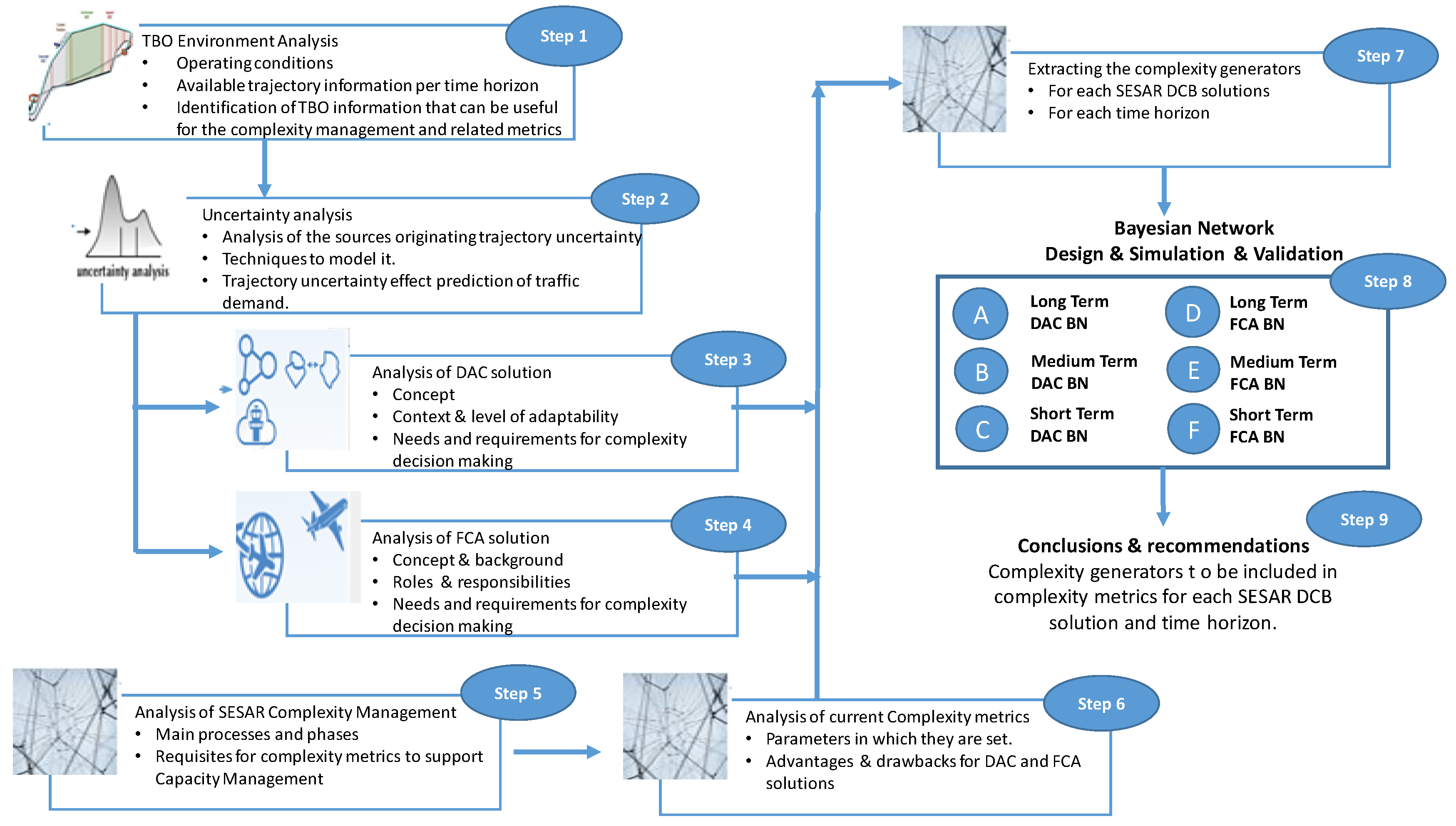
2. Materials and Methods

This research stands up on a nine steps methodology, summarized in Figure 1, and outlined hereafter:
Step 1: The first step focuses on the analysis of the TBO environment, describing the operating conditions and the trajectory information available per time horizon. Its aim is to determine what TBO information may be available and useful for complexity management.
Step 2: It consists of the study of the sources originating trajectory uncertainty; the different techniques to model it; and the evaluation of how trajectory uncertainty can affect the prediction of traffic demand.
Step 3: It analyses the DAC solution in order to contextualize what should be the purposes of the complexity metrics; and how DAC context would affect the management of complexity in each time horizon.
Step 4: It analyses the FCA solution with the same goal as in step 3. Being a concept in process of definition, different hypotheses are made, taking into account the latest results of SESAR2020 and the inputs from FCA experts.
Step 5: It implies the analysis of the main processes and phases of the “Complexity Management Process” as developed in SESAR. In this step, we extract requisites for the development of complexity metrics to support Capacity Management.
Step 6: It tackles in detail the analysis of current complexity metrics, i.e.,: the parameters in which they are set (inputs and outputs); the advantages and drawbacks of each metric; and how they could be adapted to a TBO environment, for both DAC and FCA.
Step 7: Based on the previous analysis, in this step we propose a set of “Complexity Generators” (CGs), appropriate for the different time horizons of each solution. The concept of Complexity Generators is underlying behind a certain variable considered by a mathematical model for computing complexity. Complexity Generators are identified from literature and from the studies carried out in the previous steps of the methodology; and they are tuned and validated by expert’s opinion gathered at the COTTON First Workshop. Complexity Generators are characterized in terms of their uncertainty, variability and impact on complexity metrics for each time horizon and DCB concept (DAC and FCA).
Step 8: In this step, all the previous information is used to develop and validate a Bayesian Network (BN) structure that permits to evaluate the influence of the Complexity Generators in the complexity metrics for each concept and time horizon. In particular, the network allow evaluating the impact on complexity of different levels of uncertainty in any complexity generator. In total 7 BN models are elicited covering each concept and time horizon. The networks permit also, when the required level for the uncertainty of complexity is set, to identify the complexity generators that must be used by a complexity metric to improve its degree of uncertainty to achieve that level.
Step 9: Finally, main conclusions and recommendations are obtained. Depending on the time horizon and the DCB concept, the results of the research work are:
(1)
the set of complexity generators recommended as inputs in the complexity metrics and algorithms for each application and time horizon;
(2)
the list of that would require further reduction in uncertainty; and
(3)
an evaluation of the adaptability of current complexity metrics for DAC and FCA environment.

3. Step 1. TBO Environment Analysis

In this step, the Trajectory-Based Operations (TBO) [1] concept is analysed to identify available flight information for complexity calculation and management. TBO is the based for consistent aircraft trajectory and flight information in collaborative decision-making process regarding the flight. TBO relies on the 4D trajectory concept [9].
The 4D trajectory concept implies that, long time before the departure, Estimated Elapsed Times (EET) of all waypoints along the routes are provided in the flight plan. EETs are calculated by the airline Flight Operations Centre (FOC) and the Flight Management System (FMS) considering aircraft performance, as well as weather forecast, known airspace restrictions, altitude constraints, among others. Information sharing provides a more accurate EET calculation. Tolerance Windows are associated to each EET. If EETs are added to planned take-off time, the result is a list of planned times over waypoints to landing time at the destination airport. These define the trajectory in the time dimension. After agreement by stakeholders this becomes the agreed Business Trajectory. When a flight deviates from its Business Trajectory, or planned EETs tolerance windows are not respected, the agreed Business Trajectory has to be amended requiring a recalculation of estimates over all waypoints (or part of trajectory still to be flown). The Required Time of Arrival function could be used by airspace users to comply with adherence requirements. Tolerance level can vary from the ±10 s of adherence associated with Controlled Times (CTO/CTA) to tolerance levels around a few minutes associated with Target Times (TTO/TTA). The width of the target time window is a significant element to balance flexibility versus predictability and should be carefully selected. In addition, the timing for freezing the target time plays a role in this balancing; therefore, it would equally be a parameter requiring careful selection.
Because of the previously described processes, the information available in the different phases of the planning process improves consistently the trajectories data managed by different stakeholders and decreases flight data inconsistencies. Therefore, available information need to be considered when calculating complexity. Table 1 presents an overview of the available information in each time horizon of the Network Operation Plan: Long Term planning (including airspace/route design), Medium Term planning and Short Term planning and execution.

4. Step 2: Trajectory Uncertainty Analysis

Trajectory prediction accuracy is key to get the best quality of the trajectory information and the traffic demand. However, tools and trajectory prediction models will always have certain level of uncertainty. This section overviews (i) the main sources of uncertainty in the trajectory prediction (ii) the main techniques for trajectory prediction; and finally (iii) it quantifies the impact of trajectory uncertainty on the traffic demand.

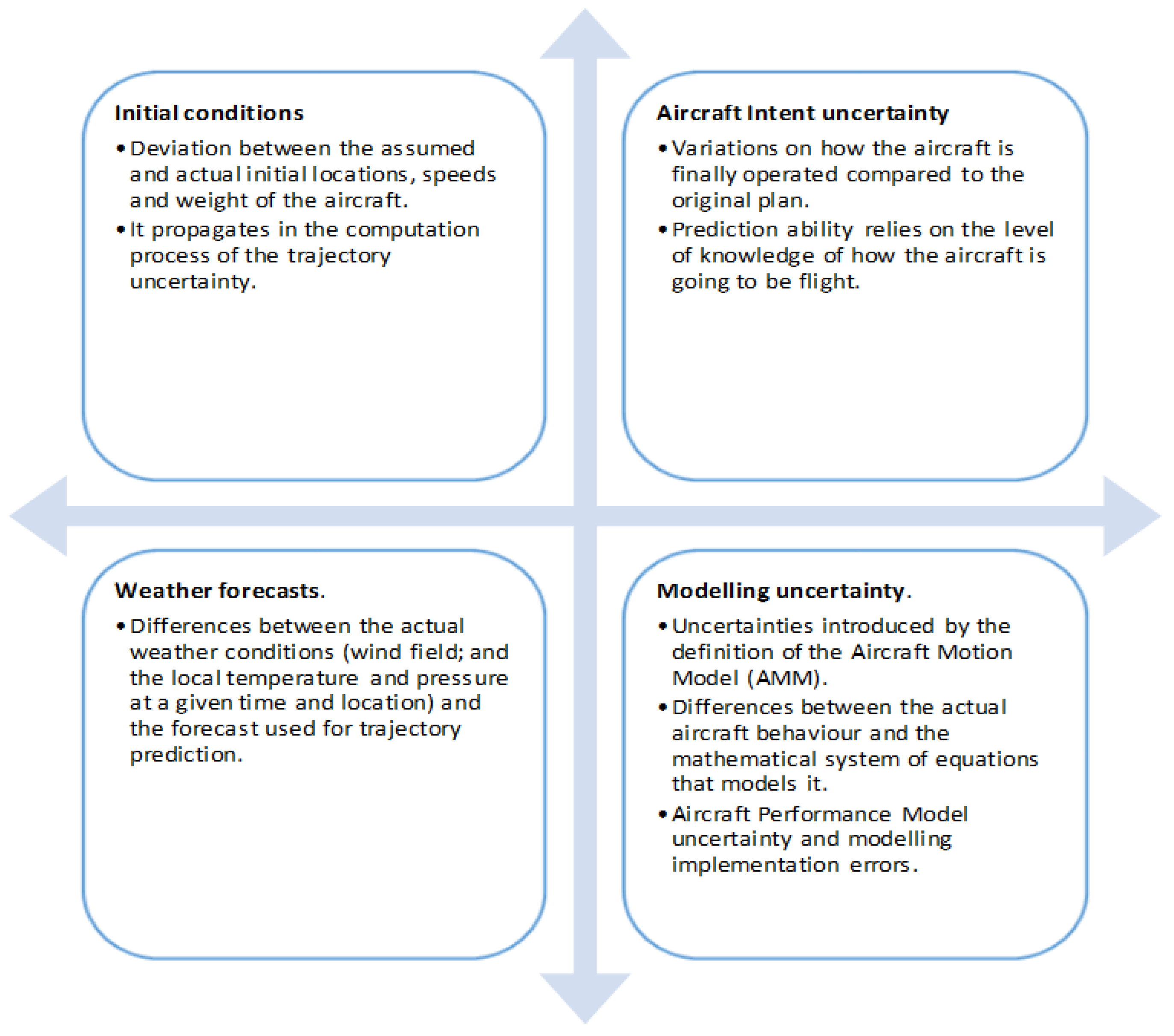
4.1. Uncertaitny Sources

When modelling aircraft trajectory, there are several factors introducing uncertainty to the trajectory computation model. Identification and characterization of the main sources of trajectory uncertainty, hereafter referred as influencing factors, will allow building an uncertainty model for complexity calculations. The latest and most advanced works in this domain have been used to drawn the main influencing factors [11,12], as illustrated in Figure 2.

4.2. Modellign Techniques

More advanced modelling techniques for incorporation of uncertainty in the trajectory prediction have been reviewed. The COPTRA project [11] considers the inputs to the trajectory prediction process as probabilistic distributions that define the nominal value of a variable and its associated uncertainty. These uncertainty distributions are estimated by analysing trajectory data with data-driven analytics methods.
The Polynomial Chaos Expansion [12] method determines the evolution of probabilistic uncertainty in a dynamical system. It characterises stochastic random variables—such as position and time—by means of polynomials of another random variables (representing the probability distributions of the uncertainty sources). Mixed-integer Linear Programming [13] methods search to minimise a linear function combination of uncertainty sources vectors, subject to constraints.
Linear Regression Approach [14] has been used to estimate the uncertainty in trajectory crossing time at a sector boundary (entry or exit) and the uncertainty in sector traffic load [15]. The technique analyses a sufficient wide data set (such as six months of operations) by comparing real data of crossing times with flight planned estimates. Monte Carlo Simulations [16] have been used to estimate the probability of compliance with tolerance windows; the generate a map of the space where aircraft can fly while avoiding conflicts with other aircraft and meeting the Target Window constraints.
In ellipsoid trajectory uncertainty modelling [17] uncertainty on trajectory is modelled by 3-dimensional ellipsoids, that represents all future aircraft locations at a certain moment in time. This method relies then on the direct characterisation of trajectory uncertainty, from real statistical aircraft data, without analysing the uncertainty sources parameters generating that final trajectory uncertainty.
Queuing models [18] characterize aircraft operations by probability distributions of service times in a queuing system. The output is the uncertainty or probability distribution of a number of pre-defined times along the trajectory/route. Aircraft and navigation performance, meteorological conditions, or ATC procedures can be mathematically modelled as queuing parameters and service time distribution. These mathematical models are then used as input to the trajectory uncertainty.

4.3. Impact of Trajectory Uncertainty on the Traffic Demand

Finally, the impact of uncertainty sources and techniques to quantify trajectory uncertainty on the traffic demand has been evaluated on the bases of SESAR PJ09 Predictive Demand Model [16] that provides a Flight Demand Forecast and identifies a Flight Demand, a Count Forecast, Imbalance Forecast, Solution Forecast and a Network Impact Forecast. Two main impacts have been identified: (i) As the time approaches to the prediction period, the accuracy of the traffic demand and occupancy prediction improves with the probabilistic traffic. The smoothing effect reduces the number of hotspot false alarms [17]; (ii) however, when the prediction time window is very far away the probabilistic traffic introduces a smoothing effect that affects negatively the hotspot detection.

5. SEPT 3: Analysis of the DAC Solution

Dynamic Airspace Configuration state of the art is studied in this section to understand how DAC context would affect the management of complexity. To that aim, the general concept and the different phases of DAC have been drawn according to SESAR1 [4] and SESAR2020 [5].
In DAC, the number and configuration of ATC sectors will adapt to the traffic pattern. The DAC process aims at identifying an optimised airspace configuration based on the complexity predicted, ATCO availability and defined performance targets. It comprises two types of processes: i) Sector Design processes supported by automation to delineate airspace structures and elementary sectors according to DAC local implementation. ii) Sector Management processes for producing the sector configuration to match the traffic for a given period. Sector Management considers multiple criteria and constraints in the search for an optimal solution: sector overload, control workload balance, traffic transfer workload, number of active sectors, etc. [19]
In DAC, complexity is used to support the selection of the designed sectors as well as the optimal airspace configuration. Conclusions of the complexity assessment will steer the sectors configuration, as well as the redistribution and allocation of human resources into sectors, to avoid an excessive workload. Table 2 highlights the four time horizons of complexity assessment in DAC solution. In the Long-term, the uncertainty of most of the input parameters is very high. Main inputs available to estimate complexity at this stage are traffic flows, demand and capacity forecasts, intentions of airspace users, etc. Long term workload evaluation can help to identify crowded areas, supporting airspace design. In the medium-term, the uncertainty of the data available is still high although decreases as the day of the operation approaches. Complexity uncertainty at this phase will be progressively reduced to better support the DAC iterative process. In the medium-term to short-term, workload evaluation will be used to update airspace configuration plan based on the available traffic information (uncertainty). DAC environment distinguishes between short-term and execution, whereas, in terms of complexity, the uncertainty of the parameters available in each of the phases is coincident.

6. SETP 4: Analysis of the FCA Solution

Similarly, Flight Centric ATC state of the art is studied to understand how FCA context would affect the management of complexity. Table 3 presents a summary of the FCA processes deconstructed.
In the FCA concept controllers are not anymore responsible for all the aircraft inside a sector; instead of that, controllers will be in charge of a set of aircraft flying within the airspace under his/her responsibility. FCA will dissolve sector boundaries in order to obtain large size airspace such as Functional Airspace Blocks (FABs), which will be designed for a suitable distribution through all European airspace.
In FCA jurisdiction, the airspace will be shared among several controllers as within the same airspace there will be more than a controller in charge of the aircraft flying through the airspace under responsibility. As each controller will be in charge of a certain number of aircraft, there have been defined two different operational environments regarding traffic allocation: dynamic allocation and static allocation. Those allocation systems will be based on the information available in each moment as well as the complexity level. In the FCA concept, traffic allocation is one of the key points related to complexity as it will determine how high controllers’ workload will be. Furthermore, a correct allocation is essential to evenly distribute workload among all active controllers. The main use of complexity metric in FCA would be for the role of Allocator and Supervisor, the first one as a tool to support flight allocation and the second to monitor the demand and capacity balancing of the whole FCA area. The workload of the flight centric executive controller is the main criteria to allocate an entering flight to FCA and secondly the potential conflicts inside FCA, then the complexity metric shall take into account these two aspects.

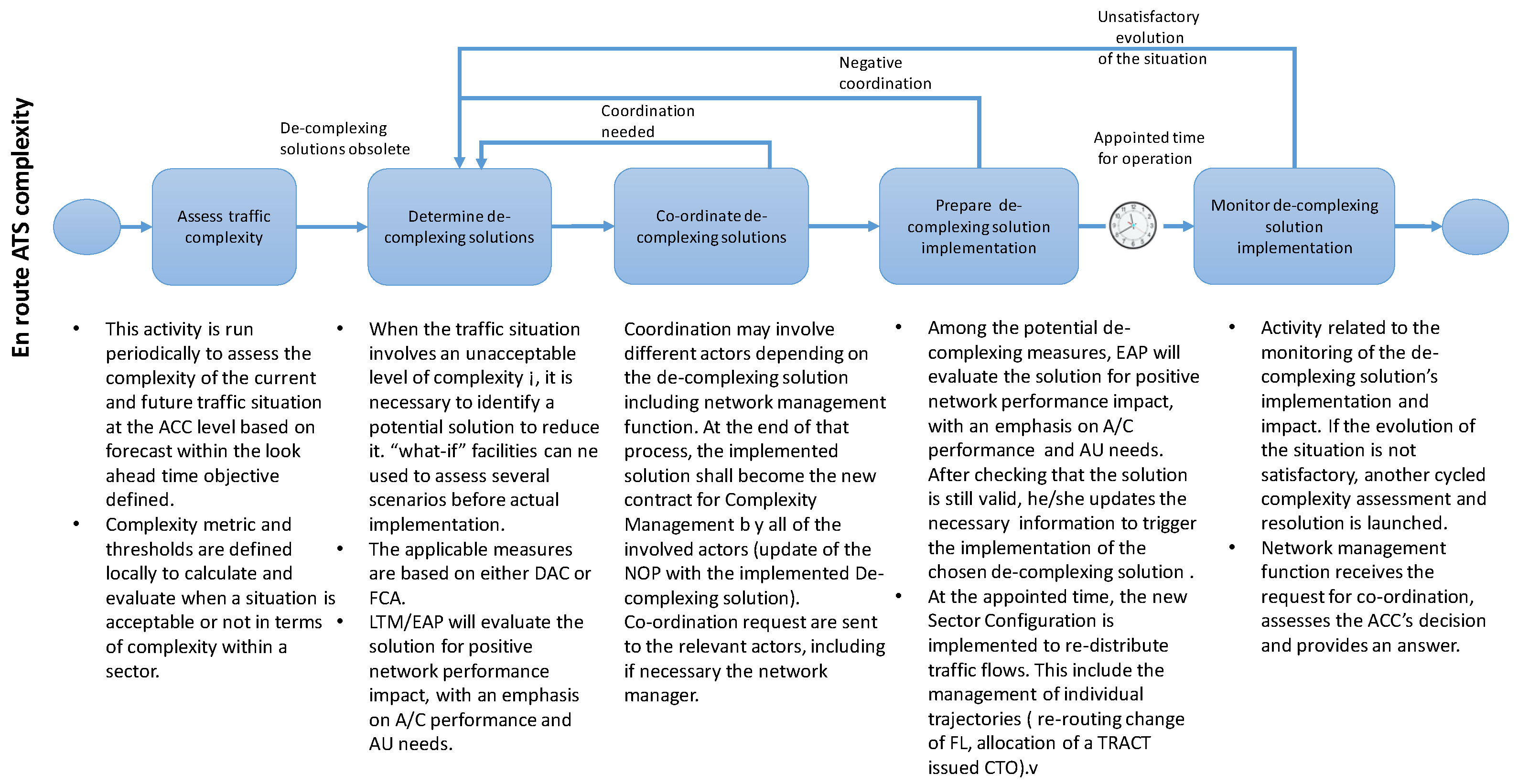
7. Step 5: Analysis of the SESAR Complexity Management

Figure 3 represents a cycle of the current SESAR traffic complexity management process, from the identification of the problem to the implementation and monitoring of the determined solution. Its analysis will allow establishing requirements and conditions that may affect the complexity methodologies and metrics for each time horizon.
After analysing the different services [7,8], processes, tools and operational environment, the main limitations for the development of metrics for complexity management can be extracted. The resolutions to air traffic complexity problems are constrained by:
  • Availability of airspace (e.g., due to weather, airspace reservation);
  • Availability of ATC sector capacity;
  • Airspace users’ preferences;
  • Air Traffic target times as results of AMAN, DMAN and Extended AMAN processes);
  • The Network stability requirements; and
  • iRBT (initial Reference Business Trajectory) and iRMT (Initial Reference Mission Trajectory) update rules.
The main constrains for the Complexity Resolution SErvice (CORSE) and (Integrated Network Management and extended ATC planning (INAP), which take place namely between 2 h and 20 min before sector entry time, are:
  • Accuracy of the input Flight Data Processing (FDP) data to be used for complexity prediction, due to the required time horizon and quality characteristics of that data;
  • Human Factors (HF) constrains related to frequent sector configuration changes;
  • Additional co-ordination procedures required by introducing of additional layer of planning without adequate automated support.
Additionally the design of adaptable complexity metrics for longer lead times (days, months) will require coarser metrics for the workload assessment, such as entry counts. It will be necessary to develop the complexity metrics that allow workload to be balanced within the DCB solutions as well.

8. STEP 6: Analysis of Current Complexity Metrics

In this step, the most promising complexity metrics are analysed to determine up to what extent their evolution and/or combination might become a solution for assessing complexity in DAC and FCA. The assessments accounts for their main characteristics, advantages, inefficiencies and limitations considering DAC and FCA solutions. In total 13 metrics have been analysed in ATM domian: 1. PHARE [20,21], 2. Fractal dimension [22], 3. Cognitive complexity metric [23], 4. Solution Space Metric [24,25], 5. Trajectory Flexibility [26], 6. Trajectory Based Complexity [27], 7. Input-Output approach [28], 8. Dynamic Density [29], 9. Geometrical approach [30], 10. Approach based on dynamical system modelling [31], 11. Trajectory uncertainty [32], 12. Probabilistic approach [33], 13. Algorithm approach [34]. Additionally complexity metrics in other industries have also been analyzed, particularly latest applications of AHP method to a multi-criteria importance analysis of complex system, as those at [35,36]. The analyses allow us to identify the most important limitations of the existing metrics:
  • They are usually not generalized and are linked to the studied sector, highly dependent on the type of algorithm used to resolve conflicts, and on specific system used to process trajectories. Whereas, in the DAC solution there will be no pre-defined sectors, and in FCA solution there will be co-existence of several controllers operating in the same airspace;
  • They are subjective and sensitive to the controllers used to infer the model since most of them focus on the opinion, behaviour, habits and subjective performance of the controller;
  • Traffic is usually managed at tactical level in the current system. However, in the new ATM system traffic complexity should support Capacity Management processes. Thus, complexity assessment should be examined to support in managing controllers’ workload;
  • They are sensitive to minor fluctuation in the traffic demand. This is more expressed with instantaneous metrics, but aggregated metrics are unstable and depend on the aggregation period (20 min, 1 h, etc.) as well. This means that uncertainty in the prediction of traffic demand have high influence at the resulting complexity level;
  • Beside the need for the complexity assessment methodology that takes into account trajectory uncertainty, there is also a need for traffic complexity metrics that takes into account system robustness. That will allow to determine how much system solution is invariant to changes in the initial conditions and external (random) influences, and be more representative of the expected traffic load and stable over the prediction time horizon;
  • Some of them are adapted for the post-operational performance evaluation or macroscopic (strategic) system evaluation, whereas, to support capacity management, metrics need to be used operationally for the real-time decision support;
Some complexity metrics provides abstract numbers that may serve for relative comparison of different solutions but are not comprehensive in expressing workload in a meaningful way to human operator. Furthermore, they are not very helpful in resolving high-workload situations, since solution for the existing problem is not obvious. It is strongly required that new metrics are comprehensible to human operator and provides indications to decision maker about the factors causing the problem and thus supporting its resolution. This requires establishing clear link between complexity and workload, and in line with this work, defining workload threshold for the new operational environments DAC and FCA.

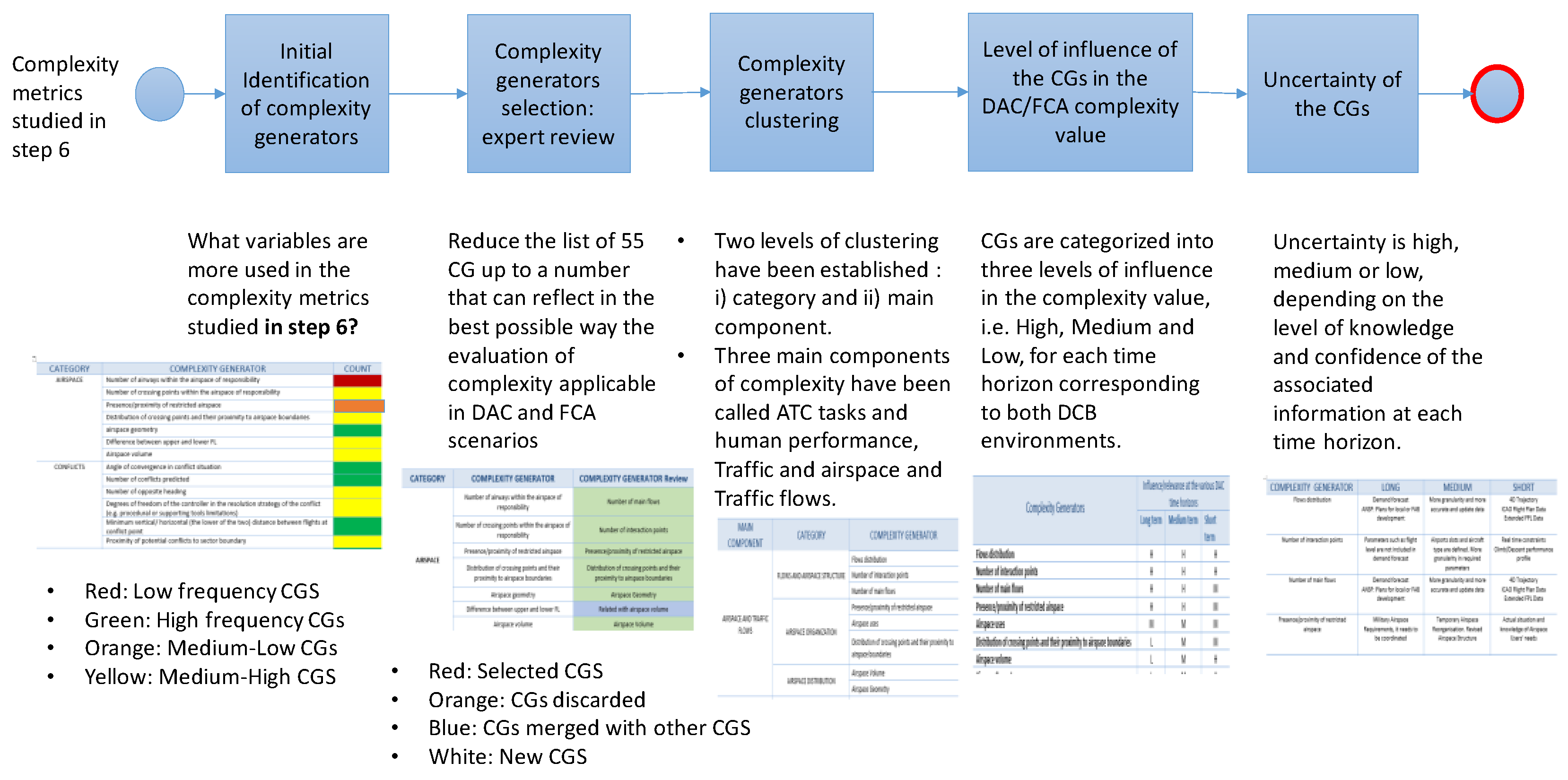
9. STEP 7: Extracting the Complexity Generators

As seen from previous sections, all complexity metrics are based on many variables to estimate the complexity associated to a specific air traffic situation. These variables catch different aspects of the air traffic or airspace from data inputs such as aircraft trajectories and sector geometry. The underlying concept behind a certain variable considered by a mathematical model for computing complexity is called a Complexity Generator (CGs). Complexity Generators are concepts instead of specific variables, which are more easily considered by ATM experts and can be adapted to any complexity metric. An example of complexity generator related to traffic distribution in a given airspace at a given time is the distribution of crossing points and their proximity to airspace boundaries. A possible associated variable would be the mean distance of all crossing points in the given airspace to the closest boundary for each crossing point.
COTTON project approach for the identification of CGs is a top-down review of existing complexity metrics (see Step 6) combined with a bottom-up analysis of complexity generators in the context of DAC and FCA. In support of this bottom-up approach, a workshop was organised with attendance of experts on complexity, trajectory optimisation, DAC and FCA concepts. The workshop addressed the identification of the CGs that have strong influence in the complexity value for each time horizon and operational concept, DAC and FCA. The selection of the most influential CGs was based on expert judgments following the method described below and summarised in Figure 4.
  • Initial identification of complexity generators. The first step for the CGs selection was to determine what variables are more used in the complexity metrics studied in step 6. Variables were translated into complexity generators, and a table was built, as shown in Figure 4, accounting for the CATEGORY (such as airspace, conflicts, flow organization…), the COMPLEXITY GENERATOR (such as airspace geometry, weather conditions, number of conflicts predicted…) and the COUNT, which indicate frequency with a colour code. This analysis doesn’t indicate what CGs are most influential to complexity but only the frequency in studied metrics. The complexity generators initial list was made up of 55 CGs.
  • Complexity Generators Selection: expert review. The aim of the first COTTON workshop was to reduce the list of 55 complexity generators up to a number that can reflect in the best possible way the evaluation of complexity applicable in DAC and FCA. A final table (see Figure 4) was produced by the experts indicating: Complexity Generators selected (green), Complexity Generators discarded (orange); Complexity Generators merged with other cgs (blue); and new Complexity Generators (white).
  • Complexity Generators Clustering. Two levels of clustering have been established: (i) category and (ii) main component. Category groups the complexity generators that may be related to specific elements in an ATM scenario. Main components symbolize states that determinate the complexity value, that is: airspace or static state, air traffic or dynamic state, and cognitive or human factors. Accordingly, the three main components of complexity have been called ATC tasks and human performance, Traffic and airspace and Traffic flows.
  • Level of Influence of the CGs in the DAC/FCA complexity value. This step aims to evaluate level of influence of complexity generators on the complexity value. Complexity generators were categorized into three levels of influence in the complexity value, i.e., High, Medium and Low, for each time horizon corresponding to both DCB environments. For the sake of illustration, Table 4 shows the level of impact of each CG in complexity value for each time horizon in the DAC concept being High influence (H), Medium influence (M) or Low influence (L).
  • Uncertainty of Complexity Generators. Uncertainty is high, medium or low, depending on the level of knowledge and confidence of the associated information at each time horizon. When approaching to the time of operation, available data will be more accurate and therefore uncertainty will be lower. Table 5 illustrates the uncertainty of each CGs at each time horizon in DAC.

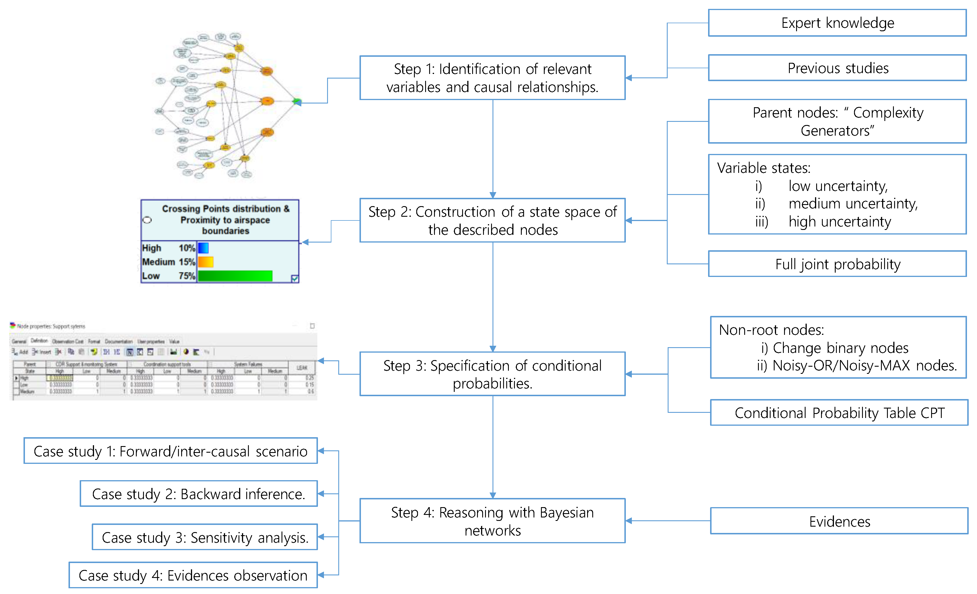
10. STEP 8: Bayesian Network Modelling

Most research up to now has approached uncertainty in TBO from the optics of uncertainty propagation methodologies (e.g., Monte Carlo simulations). This approaches construct probability distributions of the system’s outputs with numerical models that propagates probability distributions of system’s input parameters. This unidirectional propagation of uncertainties is appropriate for sensitivity analysis, although presents some limitations for backward analysis. Limitations are even greater when data are not available for the characterisation of the uncertainty of a variable, and all the information can only be elicited from expert knowledge. In such cases, the consequent backward propagation of information ought to be taken into consideration and properly modelled when using the given data to fine-tune the analysis. Limitations are not surmountable when there is no detail knowledge of the phenomena to construct a mathematical model of the process outcomes. Therefore, an alternative robust technique is proposed in this work: Bayesian Network (BN) modelling of the uncertainty propagation in the calculation of ATM complexity.
The Bayesian models relate complexity generators and their influence in ATM complexity for the two operational concepts, DAC and FCA, and the various timeframe horizons. The aim of the networks is to help to identify the relevant variables in the process, and to understand the causal relationships and interdependences between factors influencing the complexity and the uncertainties associated to those factors [37,38,39,40]. The outcome of these models is double:
  • On one side, they will help to identify what complexity generators need to be properly taken into account and analysed by the complexity algorithms and metrics adapted to the DAC and FCA concepts. Among the set of current variables considered complexity generators, the BN will help to highlight which ones are expected to have a High (H), Medium (M), or Low (L) influence in the complexity outcome itself, depending on the concept and timeframe considered. The future complexity algorithms and metrics might take this outcome as an indication of which variables, because of their influence on complexity, need to be carefully addressed by the metrics and algorithms.
  • At the same time, the networks will help to identify whether the a-priori uncertainty probability distribution of each of those variables (considering the various timeframe horizons) will be compatible with maintaining the uncertainty of complexity outcome at a LOW or MEDIUM state, or which ones will need further improvements reducing its level of uncertainty. The future complexity algorithms and metrics might take this outcome as an indication of the uncertainty they might expect for each complexity generator (High, Medium or Low), and according to that decide the best approach to characterize and measure this variable in each scenario.
A Bayesian network is a Directed Acyclic Graph (DAG), where the nodes represent random variables and the arcs describe the relationship or dependence among nodes in terms of probability [41,42]. Every node presents as set of unique and reciprocally excluding discrete or continuous values or states. Each random variable is characterized by a probability distribution. The direction of each node-to-node connection indicates a parent-child relationship. Not connected nodes accounts for conditional independence. The states of each root node are defined by marginal probabilities. Every link represents a conditional probability distribution describing the “likelihood of each value of the down-arrow node, conditional on every possible combination of values of the parent nodes” [43].
BN are build up either learning from or form knowledge and experiences. Our model aims to capture the main complexity generators as well as the relationships between them, and to explain how the level of uncertainty about the values of each complexity generator propagates and generates uncertainty in the final value of complexity. Initially, a generic model was built based on the variables and causal relationship identified from the literature survey and by the experts participating in the project. The generic Bayesian model was further adapted to each one of the operational concepts consider in the project, DAC and FCA, and to each one of its time horizons, long, medium and short term. In total seven Bayesian models were elicited using the tool GeNIe [44]. Figure 5 summarises the main steps followed for building a Bayesian Network.
Identification of relevant variables and causal relationships. The first step in the Bayesian networks construction is the identification of the relevant variables in the process to be analysed, and the assessment of the causal relationships among the variables in the. Each variable corresponds to a node in the network. The list of nodes contains the “complexity generators” identified and discussed in previous section of this paper (see Step 7), as well as some “intermediate variables” used to aggregate and integrate the effects of the complexity generators and to show how they contribute to the uncertainty in complexity. It also contains the “outcome” of the network, i.e., the “complexity”.
  • State space of each node. Next step is the construction of a state space of the described nodes, i.e., the definition of the variable states and the full joint probability of all parent nodes in the network. The state space of each parent node represents the level of uncertainty that affects a particular variable or complexity generator. The uncertainty affecting each variable has been discretised into three different states: (i) low uncertainty, (ii) medium uncertainty, and (iii) high uncertainty. Therefore, all the nodes have these three states.
  • Specification of conditional probabilities. In the following step, conditional probabilities at non-root nodes are defined, considering every potential mixture of parent nodes’ values. Conditional Probability Tables (CPTs) or distributions are employed depending whether variables are discrete and continuous. Child nodes conditional probabilities can be derived either from statistical learning or from expert knowledge elicitation [45]. In our network, conditional probabilities are derived considering the influence of each variable into its child’s specified in Step 7.
  • Reasoning and analysis. Four different case studies or inferences have been analysed for each of the Bayesian networks.
    Case study 1: Forward scenario (sometimes referred also as inter-causal analysis). The model is used to predict the effects, i.e., the uncertainty level in the complexity metric by setting the uncertainties level in the complexity generators, i.e., by setting the probability distribution of the parent-input nodes. This case study is useful to answer the following research question: Given the probability distribution of the uncertainty of the various complexity generators, how these uncertainties propagate through the network causing a probability distribution for the uncertainty (% of high uncertainty, % of medium uncertainty or % of low uncertainty) in the outcome of the network, “complexity”? This is a typical prediction scenario.
    Case study 2: Backward inference. The model is used to deliver the parent’s node configuration by setting the outcome node (uncertainty level of the complexity metric) to a target value. In this analysis complexity uncertainty is successively settled to a high, medium or low value. Then, the network identify the main contributors to the value of complexity uncertainty, or what configuration of uncertainty might be admitted at the various complexity generators to provide the target outcome uncertainty. This case study is useful to answer the following questions: how much will it be necessary to improve uncertainty in the inputs nodes to achieve a certain uncertainty level in the outcome node?; or what will be the probability of any fault (uncertainty level of the input nodes) given a set of symptoms or results (uncertainty level of the outcome)? This is a typical fault diagnosis scenario.
    Case study 3: Sensitivity analysis. It is used to investigate the impact of small variations in input parameters probabilities eon the posterior probabilities of the output parameters.
    Case study 4: Evidences observation. As far as detailed characterization of the uncertainty of a variable is observed (high, medium or low uncertainty), the evidence can be pictured as propagated through the network. Then the network can be updated with such evidence, and the conditional probabilities of the rest of the variables, including the outcome are recalculated. These new values allow us to evaluate how much improvement can be achieving in reducing the uncertainty of the network outcome by improving the uncertainty related to one or some of the complexity generators.

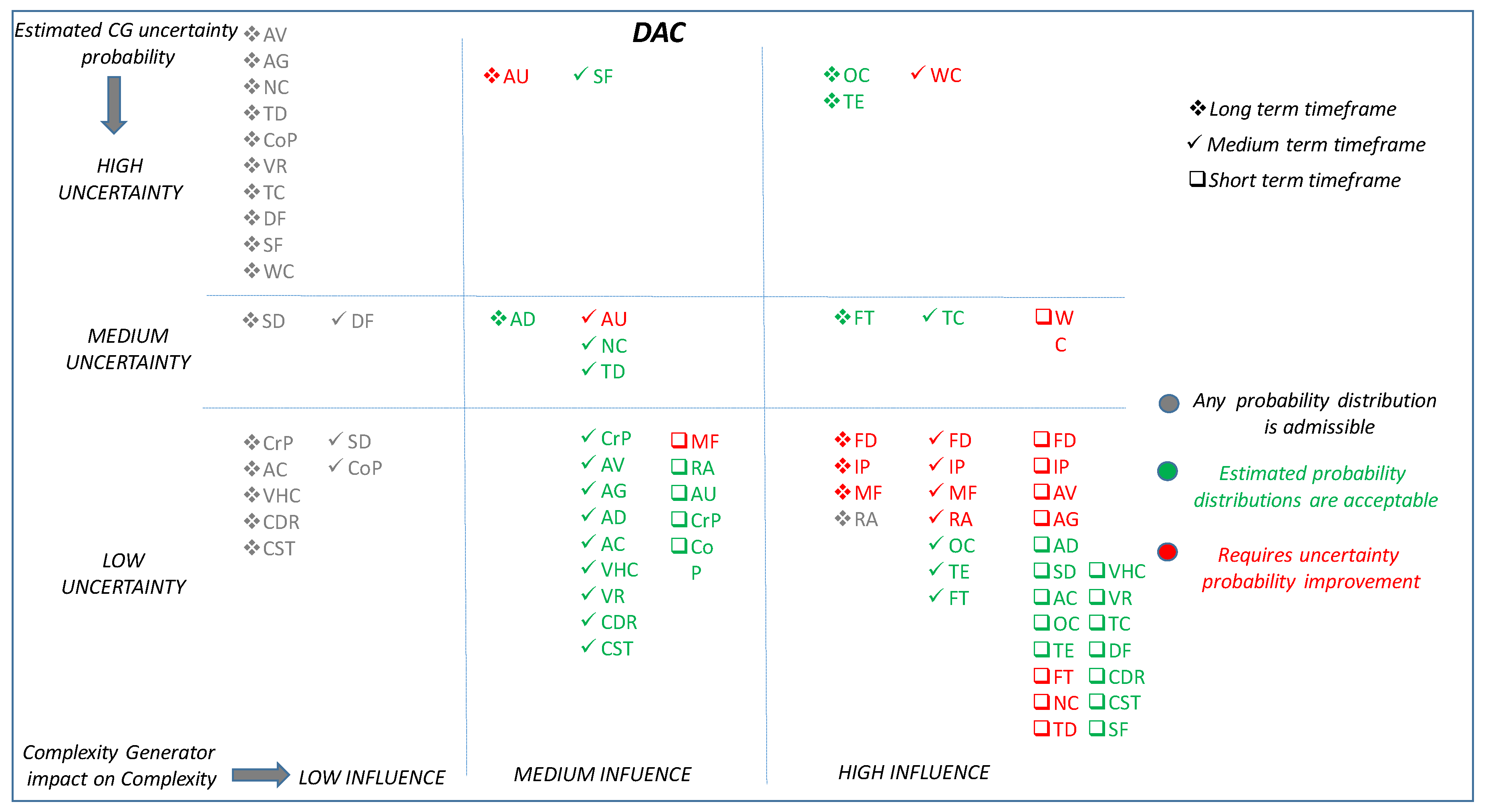
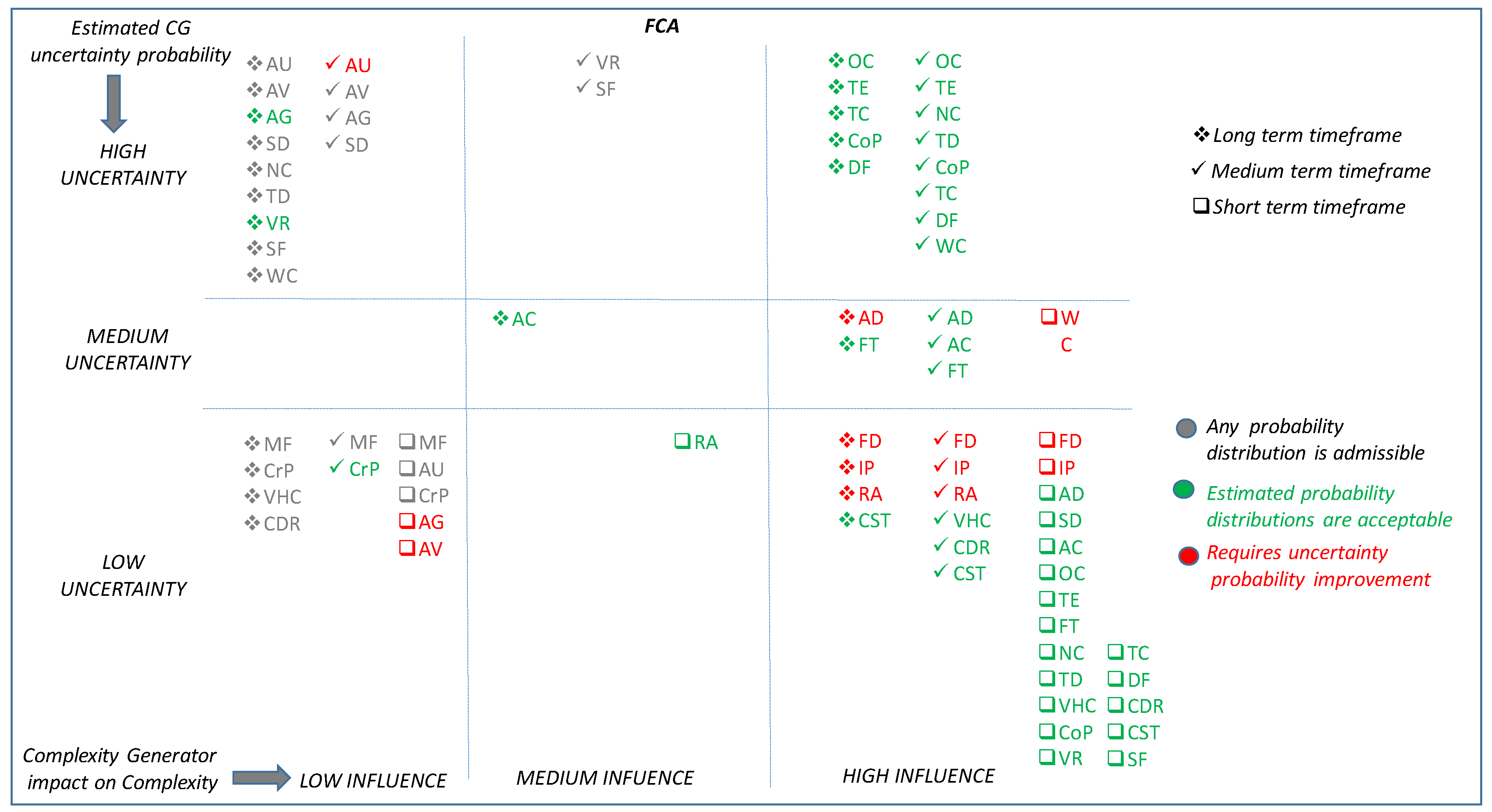
11. Step 9: Discussion of Results

Figure 6 and Figure 7 summarise, in a multidimensional diagram, the conclusions derived from the previous analysis, particularly from the BN case studies. They present for each application the pool of preferred/recommended candidates to be used as complexity generators in each time horizon. Rationale behind both of them is explained hereafter:
  • First, the complexity generators have been classified according to: (i) their level of influence on global complexity, in the horizontal dimension of the diagram; and (ii) their degree of uncertainty of the information, in the vertical dimension of the diagram.
  • Following these criteria, the diagram is divided into nine regions of different influence on complexity and degree of uncertainty. For example, complexity generators placed on the bottom right corner of the diagram have high influence on complexity and a low degree of uncertainty associated to its information.
  • Once the complexity generators have been classified, a colour code has been defined to reflect the results of the analysis. Red: Requires an improvement in the level of uncertainty of the information estimated for this generator, in the considered time horizon. Green: The estimated level of uncertainty may be acceptable to maintain final objectives of uncertainty in complexity. Grey: The uncertainty level does not impact the final result due to the low influence of the parameter.
  • Finally, in the figure, each one of the time horizons considered is reflected with a different symbol: □ Short Term, √ Medium Term, and * Long Term.
Table 6 shows the acronyms code used in the figure to represent each Complexity Generator.
Complexity generators that have high influence on “complexity”, should conform the pool of preferred candidates to be measured, quantified, and evaluated by the complexity metrics and algorithms. These ones are placed in the right hand side column of the multidimensional diagram. Complexity generators with low influence are considered a priori less suitable parameters for the complexity metrics and algorithms. These ones are placed in the left hand side column of the multidimensional diagram. Finally, those with medium influence might deserve detailed and individual consideration to evaluate up to what extent they contribute to the complexity algorithms and metrics, depending upon the demand and capacity balance application and timeframe, and the uncertainty with which each variable is known. These ones are located in the central column of the multidimensional diagram.
In relation to the results established in Figure 6, the following conclusions are drawn for the DAC application: a close look at the high influence complexity generators shows that the pool of preferred candidates is bigger in the short term. In the long term, most complexity generators have a low influence on the complexity assessment (those 16 located in the left column of the multidimensional diagram), complemented mostly by a high associated uncertainty, with 8 out of the 25 complexity generators placed on the top left corner of the diagram. It can also be seen in the multidimensional diagram, that some of the complexity generators which have a high influence in the long term, either have a high associated uncertainty (two out of seven) or need to improve their uncertainty probability distribution (three out of seven). Therefore, the range of options for preferred candidates in the long term is small. Whereas, in the short term, 19 out of the 25 variables are well placed in the bottom-right corner of the diagram, constituting a bigger pool of recommendable candidates a priori. In the DAC diagram, a progressive migration of the variables towards higher influences and lower uncertainties is observed through the time horizons, from the long to the short time frame. Most of the variables are qualified either as low or high uncertainty, and only a few are considered with a medium level of uncertainty, particularly in the medium time frame. This can be easily observed in the central raw of the diagram.
For complexity metrics and algorithms that focus on the medium term of the DAC application, the pool of preferred candidates is bigger than in the long term. In addition, in the medium term, nine complexity generators are characterised by an acceptable probability distribution, low uncertainty and medium influence. These variables should be carefully considered by the complexity metrics and algorithms, since they could be a useful complement to those parameters selected in the first place because to their high influence.
In the short term, there are no parameters in the low influence column, because the impact of Complexity Generators in the short term is mostly high and there is more precise information about them due to the proximity to operation, so the majority of the complexity generators are located in the lower right box of the diagram.
Regarding the overall DAC application, it can be observed that two variables, Flows Distribution and Number of Interaction Points, are important through the three time horizons, but both need to reduce their uncertainty. This fact suggests that one of the recommended lines of work could be to improve the information regarding these parameters in all time horizons.
Other variables, which are important in all time horizons and should be taken into account throughout the entire process, are: Occupancy, Traffic Entries and Distribution of flight time per aircraft under ATCO responsibility in the given timeframe. However, it will be important to bear in mind that these generators have greater associated uncertainty in the long term, so it is recommendable reduce the uncertainty associated to this variable in the long term, so that this variable could be considered an acceptable parameter for all the time horizons.
Following equivalent principles, overall conclusions and recommendations for the FCA application are drawn hereafter. A first look to Figure 7 corroborates that there are certain trends common to both applications, DAC and FCA:
  • A big set of the complexity indicators in the long term have a low influence on the complexity assessment, and at the same time high uncertainty, and consequently the range of options for preferred candidates in the long term is also small for FCA.
  • The pool of preferred candidates, those having high influence and low uncertainty, is also bigger in the short.
  • Most of the variables are qualified either as low or high uncertainty, and only a few are considered with a medium level of uncertainty, although in the FCA case, the few ones with medium uncertainty are considered mostly of high influence.
There are also some facts that differs in the FCA case:
  • In the FCA diagram only a few number of variables is considered with medium influence, maximum two out of 25. The distribution of variables between low and high influence is more extreme that for the DAC. This can be easily noticed as the intermediate column in the diagram is almost empty.
  • The number of variables requiring uncertainty reduction is lower in the short time frame for the FCA application.
For the medium and long time horizons the split of variables with high influence according to its uncertainty level, is more homogeneous than for the DAC case. The number of variables with low influence and high uncertainty is considerable for both time horizons, medium and long. The higher the effort on reducing the uncertainty associated to these variables, the higher the number of preferred candidates will be.
In the short term, the majority of the complexity generators are located in the lower right box of the diagram (high influence and low uncertainty), and just a few (five of 25) are considered of low influence. The pool of preferred candidates for FCA in the medium term is also bigger than in the long term.
As an overall issue also for the FCA application, Flows Distribution and Number of Interaction Points, are important through the three time horizons and both need to reduce their uncertainty. Therefore, the recommendation made for DAC, to improve the information regarding these parameters in all time horizons, is also valid for the FCA application.
As a final summary, Table 7 presents the set of complexity generators recommended as inputs in the complexity metrics and algorithms for each application and time horizon. Those highlighted in bold would require further reduction in uncertainty before being used in complexity metrics.
Taking into account these recommendations and the Complexity Generators that use each of the analysed metrics, three levels of difficulty are presented in Table 8, that imply a greater or lesser facility to adapt each of the metrics to the indicated scenario.
The three levels of difficulty are indicated with a color code:
-
Cells marked in green stand for the metrics that can be easily adapted to the conditions of that time horizon.
-
Cells marked in yellow represent the intermediate level of difficulty.
-
Cells marked in orange corresponds to those whose adaptation to the temporal horizon would require a greater level of effort, taking into account the recommendations made previously.
Therefore, project efforts will focus on adapting metrics that can deliver results with less effort in the identified scenarios.

12. Conclusions

The main objective of the COTTON project is to deliver innovative solutions to maximize the performance of the Capacity Management exploiting the trajectory information available in a TBO environment. In this context, the principal aim of this work was to address the challenge of exploring how the uncertainties associated with the agreed trajectory will influence the quality of the predictions of complexity of traffic demand and the effectiveness of DCB processes regarding airspace management.
To achieve this aim we have developed and implemented an ad-hoc methodology combining qualitative and quantitative approaches that integrates the state of the art of SESAR works on complexity, experts’ knowledge and advanced causal and predictive BN models. Instead of starting from scratch, research has taken full advantage of existing complexity methodologies as well as innovative models for the prediction of trajectories’ uncertainty, focusing its effort on researching how these models and methodologies can integrate the delivery of uncertainty-based complexity assessment as part of an advanced demand/capacity model. This approach has been feasible as COTTON has full access to existing SESAR complexity methodologies (Algorithm approach, Cognitive approach and Convergence-Lyapunov approach) and trajectories’ uncertainty models thanks to the composition of its Consortium. This has allowed us to explore the opportunities to refine these models introducing new trajectory-based complexity metrics for supporting the most demanding features of DAC and FCA.
The characteristics of the operational concept TBO that will influence the uncertainty of the trajectory have been identified. The analysis of the TBO environment highlighted available information need to be considered when calculating complexity in each time horizon of the Network Operation Plan.
Likewise, the characteristics of the DAC and FCA applications that can affect complexity management processes have been analysed to contextualize: (i) what should be the purposes of the complexity metrics; and (ii) how DAC context would affect the management of complexity in each time horizon. A deep look at the cycle of the current SESAR traffic complexity management process has allowed establishing requirements and conditions that may affect the complexity methodologies and metrics for each time horizon.
We have also performed a detailed survey of current complexity methods and metrics in order to identify the parameters in which they are set (inputs and outputs); the advantages and drawbacks of each metric; and how they could be adapted to a TBO environment, for both DAC and FCA. This analyses allowed also to identify the most important limitations of the existing metrics:
From the trajectory uncertainty analysis, we have identified the main sources of uncertainty in the trajectory prediction and the main techniques for trajectory prediction; and finally we have quantified the impact of trajectory uncertainty on the traffic demand.
Main research outcomes includes the identification of the key elements for the definition of complexity in the Capacity Management applications (called Complexity Generators). The concept of Complexity Generators is underlying behind a certain variable considered by a mathematical model for computing complexity. Complexity Generators are identified from literature and from the studies carried out in the previous steps of the methodology; and they are tuned and validated by expert’s opinion gathered at the COTTON First Workshop. Complexity generators have been characterised in terms of their uncertainty, variability and impact on complexity metrics for each time horizon and DCB concept (DAC and FCA).
Then, causal predictive models have been developed, using Bayesian Networks, to evaluate the effect of trajectory uncertainty on complexity assessment. The aim of the networks is to help to identify the relevant variables in the process, and to understand the causal relationships and interdependences between factors influencing the complexity and the uncertainties associated to those factors. In total 7 BN models have been elicited covering each concept and time horizon.
The outcome of these BN models was double. On the one hand, they will help to identify what Complexity Generators need to be properly taken into account and analysed by the complexity algorithms and metrics adapted to the DAC and FCA concepts. Among the set of current variables considered complexity generators, the BN will help to highlight which ones are expected to have a High (H), Medium (M), or Low (L) influence in the complexity outcome itself, depending on the concept and timeframe considered. The future complexity algorithms and metrics might take this outcome as an indication of which variables, because of their influence on complexity, need to be carefully addressed by the metrics and algorithms. At the same time, the networks will help to identify whether the a-priori uncertainty probability distribution of each of those variables (considering the various timeframe horizons) will be compatible with maintaining the uncertainty of complexity outcome at a LOW or MEDIUM state, or which ones will need further improvements reducing its level of uncertainty. The future complexity algorithms and metrics might take this outcome as an indication of the uncertainty they might expect for each complexity generator (High, Medium or Low), and according to that decide the best approach to characterize and measure this variable in each scenario.

Author Contributions

Conceptualization, R.M.A.V., V.F.G.C., A.V., M.S.C. and S.Z.; methodology, R.M.A.V., V.F.G.C.; validation, R.M.A.V., V.F.G.C., A.V., M.S.C. and S.Z.; formal analysis, R.M.A.V., V.F.G.C., A.V. M.S.C. and S.Z. investigation, R.M.A.V., V.F.G.C., A.V., M.S.C. and S.Z.

Funding

This paper presents research conducted within COTTON project (Grant 763807) sponsored by the SESAR Joint Undertaking as part of SESAR 2020 Exploratory Research Programme and conducted within EU’s Horizon 2020 research and innovation programme.

Conflicts of Interest

The authors declare no conflict of interest.

Nomenclature

List of Symbols
FDFlows Distribution
IPNumber of interaction points
MFNumber of main flows
RAPresence/proximity of restricted airspace
AUAirspace uses
CrPDistribution of crossing points and their proximity to airspace boundaries
AVAirspace volume
AGAirspace Geometry
ADAltitude AC distribution
SDSpeed AC distribution
ACAltitude AC changes
OCOccupancy (per ATCO position)
TETraffic Entry (per ATCO position)
HHigh influence
MMedium influence
LLow influence
FTDistribution of flight time per aircraft under ATCO responsibility in the given timeframe
NCNumber of conflicts predicted
TDTime difference at crossing points
VHCVertical and horizontal convergence
CoPCoordination procedures
VRVectoring and operational restrictions
TCTransition and changes in configuration
DFDegrees of freedom of the controller in the resolution strategy of the conflict
CDRCDR Support and monitoring System
CSTCoordination support tools
SFSystem failure
WCWeather conditions
Energies 12 01559 i001Short term timeframe
Energies 12 01559 i002Medium term timeframe
Energies 12 01559 i003Long term timeframe
List of Acronyms
ADEPAirport of DEStination
ADESAirport of DEParture
AMANArrival MANager
ANSPsAir Navigation Service Providers
ATCOAir Traffic Controller
ATMAi Traffic Management
BNBayesian Network
CDMCollaborative Decision Making
CDRConDitional Route
CGsComplexity Generators
COPTRACombining PRObable TRAjectories
CTO/CTAControlled Time Over/At
DACDynamic Airspace Configuration
DAGDirected Acyclic Graph (),
DCBDemand Capacity Balance
DMANDeparture MANagers
CORSEComplexity Resolution Service
EETEstimated Elapsed Times
EUEuropean Union
FCAFlight Centric ATC
FDPFlight Data Processing
FMSFlight Management System
FPLFlight Plan Level
FOCFlight Operations Centre
GUFIGlobal Unique Flight Identifier
HFHuman Factors
IATA International Airline Traffic Association
INAPIntegrated Network Management and extended ATC planning
iRBTinitial Reference Business Trajectory
iRMTInitial Reference Mission Trajectory
NPRNominal Preferred Route
TTA=/TTATarget Times Over/At
SESAR 2020Single European Sky ATM Research
SBTShared Business Trajectory
RBTReference Business Trajectory
TBOTrajectory Based Operations
TMATerminal Area Manoeuvring

References

  1. ICAO. TBO Concept; ICAO: Montreal, QC, Canada, 2015. [Google Scholar]
  2. Sesar Joint Undertaking. SESAR2020, SESAR PJ09 OSED, 00.01.00 ed.; SESAR: Brussels, Belgium, 2017. [Google Scholar]
  3. Sesar Joint Undertaking. SESAR ConOPs at a Glance, 02.00.00 ed.; SESAR: Brussels, Belgium, 2011. [Google Scholar]
  4. Guichard, L.; Garnham, R.; Zerrouki, L.; Schede, N. Dynamic Airspace Configuration Step 2-V2 OSED; SESAR: Brussels, Belgium, 2016. [Google Scholar]
  5. Sergeeva, M.; Delahaye, D.; Zerrouki, L.; Schede, N. Dynamic Airspace Configurations Generated by Evolutionary Algorithms. In Proceedings of the 34th Digital Avionics Systems Conference, Prague, Czech Republic, 13–17 September 2015. [Google Scholar]
  6. SESAR Jont Undertaking. SESAR Solution PJ.10-01b (Flight Centred ATC) Intermediate SPR-Interop/OSED for V1—Part I; SESAR: Brussels, Belgium, 2018. [Google Scholar]
  7. Terzioski, P.; Cano, M.; Llorente, R. STEP1 V3 Final Complexity Management SPR; SESAR: Brussels, Belgium, 2016. [Google Scholar]
  8. Cano, M.; Terzioski, P.; Llorente, R.; Gómez, J. STEP1 V3 Final Complexity Management OSED; SESAR: Brussels, Belgium, 2016. [Google Scholar]
  9. Hof, H.; Flohr, R.; Nunez, O.; Garr, R. Time Adherence in TBO; ATMRPP-WG/27-WP/636, ICAO—AIR Traffic; Management Requirements and Performance Panel (Atmrpp): Montreal, QC, Canada, 2014. [Google Scholar]
  10. Radišić, T.; Radišić, T. The Effect of Trajectory-Based Operations on Air Traffic Complexity. Ph.D. Thesis, Faculty of Transport and Traffic Sciences, Sveučilište u Zagrebu, Zagreb, 2014. [Google Scholar]
  11. COPTRA. Techniques to Determine Trajectory Uncertainty and Modelling; SESAR: Brussels, Belgium, 2016. [Google Scholar]
  12. Casado, E.; la Civita, M.; Vilaplana, M. Quantification of Aircraft Trajectory Prediction Uncertainty Using Polynomial Chaos Expansions. In Proceedings of the IEEE/AIA 36th Digital Avionics Systems Conference, St. Petersburg, FL, USA, 17–21 September 2017. [Google Scholar]
  13. Franco, A.; Rivas, D.; Valenzuela, A. Optimal Aircraft Path Planning Considering Wind Uncertainty. In Proceedings of the 7th European Conference for Aeronautics and Space Sciences, Milan, Italy, 3–6 July 2017. [Google Scholar]
  14. Zhu, K.; Wang, J.; Mitchell, T.; Supamusdisukul, T. Pre-Departure Stochastic Trajectory Modeling and Its Calibration with Oceanic Operational Data. In Proceedings of the 12th AIAA Aviation Technology, Integration, and Operations (ATIO) Conference, Indianapolis, Indiana, 17–19 September 2012. [Google Scholar]
  15. Mueller, T.; Sorensen, J.; Couluris, G. Strategic aircraft trajectory prediction uncertainty and statistical sector traffic load modelling. In Proceedings of the AIAA Guidance, Navigation and Control Conference, Monterrey, CA, USA, 5–8 August 2002. [Google Scholar]
  16. Margellos, K.; Lygeros, J. Toward 4D Trajectory Management in Air Traffic Control: A Study Based on Monte Carlo Simulation and Reachability Analysis. IEEE Trans. Control Syst. Technol. 2013, 21, 1820–1833. [Google Scholar] [CrossRef]
  17. Knorr, D.; Walter, L. Trajectory uncertainty and the impact on sector complexity and workload. In SESAR Innovation Days; SESAR: Brussels, Belgium, 2011. [Google Scholar]
  18. Kim, J.; Tandale, M.; Menon, P.K. Modeling Air-Traffic Service Time Uncertainties for Queuing Network Analysis. IEEE Trans. Aerosp. Electron. Syst. 2012, 48, 525–541. [Google Scholar]
  19. Sergeeva, M. Automated Airspace Sectorization by Genetic Algorithm. Optimization and Control. Ph.D. Thesis, Université Paul Sabatier, Toulouse, France, 2017. [Google Scholar]
  20. Meckiff, C.; Chone, R.; Nicolaon, J.P. The Tactical Load Smoother for Multi-Sector Planning. In Proceedings of the USA/Europe Air Traffic Management R&D Seminar, Orlando, FL, USA, 1–4 December 1998. [Google Scholar]
  21. Whiteley, M. PHARE Advanced Tools—Tactial Load Smoother; Eurocontrol: Brussels, Belgium, 1999. [Google Scholar]
  22. Liang, D.; Mondoloni, S. Airspace fractal dimension and applications. In Proceedings of the USA/Europe Air Traffic Management R&D Seminar, FAA&EUROCONTROL, Santa Fe, NM, USA, 4–7 December 2011. [Google Scholar]
  23. Comendador, V.F.G.; de Frutos, P.L.; Puntero, E.; Ballestín, E.L.; Cañas, J.J.; Ferreiras, P.; Valdes, R.A.; Sanz, A.R. An ATCo Psychological Model with Automation. In Proceedings of the 7th EASN International Conference, Warsaw, Poland, 26–29 September 2017. [Google Scholar]
  24. Hermes, P.; Mulder, M.; van Paassen, M. Solution-Space-Based Analysis of the Difficulty of Aircraft Merging Tasks. J. Aircr. 2009, 46, 1995–2015. [Google Scholar] [CrossRef]
  25. D’Engelbronner, J.; Borst, C.; Ellerbroek, J.; van Paassen, M.; Mulder, M. Solution-Space Based Analysis of Dynamic Air Traffic Controller Workload. J. Aircr. 2015, 52, 1146–1160. [Google Scholar] [CrossRef]
  26. Idris, H.; Delahaye, D.; Wing, D. Distributed Trajectory Flexibility Preservation for Traffic Complexity Mitigation. In Proceedings of the Eighth USA/Europe Air Traffic Management Research and Development Seminar (ATM2009), Napa, CA, USA, 29 June–2 July 2009. [Google Scholar]
  27. Prevot, T.; Lee, P. Trajectory-Based Complexity (TBX): A modified aircraft count to predict sector complexity during trajectory-based operations. In Proceedings of the IEEE/AIAA 30th Digital Avionics Systems Conference, Seattle, WA, USA, 16–20 October 2011. [Google Scholar]
  28. Prandini, M.; Piroddi, L.; Puechmorel, S.; Bráz, S. iFly D3.1., Complexity Metrics Applicable to Autonomous Aircraft; SESAR: Brussels, Belgium, 2009. [Google Scholar]
  29. Laudeman, I.; Shelden, S.; Branstrom, R.; Brasi, C. Dynamic Density: An Air Traffic Management Metric, NASA-TM-1998-112226; NASA: Moffet Field, CA, USA, 1999.
  30. Delahaye, D.; Puechmorel, S. Air traffic complexity: Towards intrinsic. In Proceedings of the USA/Europe Air Traffic Management R&D Seminar, Napoli, Italy, 3–6 June 2000. [Google Scholar]
  31. Delahaye, D.; Puechmorel, S.; Delahaye, D.; Puechmorel, S. Air Traffic Complexity Versus Control Workload. In Proceedings of the EuroGNC, European Aerospace Guidance, Navigation and Control Conference 2015, Toulouse, France, 13–15 April 2015. [Google Scholar]
  32. Walter, L.; Pusch, M.; Holzapfel, F.; Knorr, D. Quantifying Trajectory Uncertainty Using a Sensitivity-Based Complexity Metric Component. In Proceedings of the ICRAT-2010, Budapest, Hungary, 1–4 June 2010. [Google Scholar]
  33. Prandini, M.; Hu, J.; Putta, V. Air Traffic Complexity in Future Air Traffic Management Systems. J. Aerosp. Oper. 2012, 1, 281–299. [Google Scholar]
  34. SESAR Joint Undertaking. STEP 1 Consolidation of Previous Studies; SESAR: Brussels, Belgium, 2010. [Google Scholar]
  35. Chybowski, L.; Gawdzińska, K. On the possibilities of applying the AHP method to multi-criteria component importance analysis of complex technical objects. New Adv. Inf. Syst. Technol. 2012, 445, 701–710. [Google Scholar]
  36. Chybowski, L.; Twardochleb, M.; Wiśnic, B. Multi-criteria Decision making in Components Importance Analysis applied to a Complex Marine System. Int. J. Marit. Sci. Technol. 2016, 63, 264–270. [Google Scholar]
  37. Korn, C.; Bernd, B. Sectorless Atm–Analysis and simulation results. In Proceedings of the 27th International Congress of the Aeronautical Sciences, Nice, France, 19–24 September 2010. [Google Scholar]
  38. Sanz, A.R.; Comendador, V.F.G.; Valdés, R.M.A. Uncertainty Management at the Airport Transit View. Aerospace 2018, 5, 59. [Google Scholar] [CrossRef]
  39. Valdes, R.M.A.; Chen, S.Z.L.; Comendador, V.F.G. Application of Bayesian Networks and Information Theory to Estimate the Occurrence of Mid-Air Collisions Based on Accident Precursors. Entropy 2018, 20, 969. [Google Scholar]
  40. Valdés, R.M.A.; Comendador, V.F.G.; Sanz, L.P.; Sanz, A.R. Prediction of aircraft safety incidents using Bayesian inference and hierarchical structures. Saf. Sci. 2018, 104, 216–230. [Google Scholar] [CrossRef]
  41. Pearl, J. Probabilistic Reasoning in Intelligent Systems; Morgan Kauffman: San Mateo, CA, USA, 1998. [Google Scholar]
  42. Norvig, P.; Stuart, R. Artificial Intelligence: A modern Approach, 2nd ed.; Pearson Education, Inc.: Upper Saddle River, NJ, USA, 2003. [Google Scholar]
  43. Borsuk, M.E.; Stow, C.A.; Reckhow, K.H. A Bayesian network of eutrophication models for synthesis, prediction, and uncertainty analysis uncertainty analysis. Ecol. Model. 2004, 173, 219–239. [Google Scholar] [CrossRef]
  44. BayesFusion. GeNIe Modeler, Version 2.2; GeNIe Modeler, BayesFusion, LLC: Pittsburgh, PA, USA, 2017.
  45. Cooke, N. Varieties of knowledge elicitation techniques. Int. J. Hum. Comput. Stud. 1994, 41, 6801–6849. [Google Scholar] [CrossRef]
Figure 1. Cotton Methodology.
Energies 12 01559 g001
Figure 2. Influencing factors.
Energies 12 01559 g002
Figure 3. Manage Traffic Complexity.
Energies 12 01559 g003
Figure 4. Extracting the Complexity Generators (CGs).
Energies 12 01559 g004
Figure 5. Steps in the construction of a generic Bayesian Network for complexity.
Energies 12 01559 g005
Figure 6. Overall situation for Complexity Generators. DAC application.
Energies 12 01559 g006
Figure 7. Overall situation for Complexity Generators. FCA application.
Energies 12 01559 g007
Table 1. Information available per time horizon.
Trajectory Based Operations
LONG-TERMMEDIUM-TERMSHORT-TERMEXECUTION PHASE
From 5 years up to 6 months6 months until one weekOne week to 24 hDay of operations
DATADATADATADATA
Routing Preference (historical data) and PrioritiesShared Business Trajectory (SBT) Scheduling Phase4D trajectory planning phase. ATM Short-termReference Business Trajectory (RBT)
Agreed performance targets for capacity and flight efficiency at network and local level Scheduled data
IATA flight Identification
ADEP
ADES
Schedule time of departure
Schedule time of arrival
Aircraft type
Period of operations
Days of operations
ICAO Flight Plan DataGlobal Unique Flight Identifier (GUFI)
Existing Airspace StructureGlobal Unique Flight Identifier (GUFI)Extended FPL Data
Airspace Availability/Conditions of Use Departure runwayReal time constraints or ATC constraints
Default Airspace Availability Arrival runwayDCB measures and tolerances
Identified capacity bottlenecks DCB measures and tolerancesTSAT/TTOT
Coordination of airspace design plans (local/sub-regional) 4D Trajectory
Taxi-time
Air trajectory
Location
Latitude and longitude
Previous route segment
Level
Elapse time from take-off up to the location
Distance
Total weight
True air speed
Target Time applied (if has been published.)
Minimum Altitude
Maximum altitude
Probability Sigma
ANSP: Plans for local or FAB development Nominal Preferred Route (NPR)
Airport slots
Table 2. Dynamic airspace configuration description in ATM processes.
ATM ProcessTime LineSpecific ProcessesDescription
Long Term Process From years to 3 daysAnalyze Network performance and airspace organization/configuration needs, particularly those concerned with airspace design and resourcesAirspaces is designed to enable dynamic configurations to be used, and the ATM resources are made available to use the requires airspace configuration
Medium Term ProcessFrom 6 month to 3 daysCollaboratively update and publish airspace configuration plan and develop an optimum airspace configuration
Short Term Process From 3 days to hours The processes in medium and short term are broadly similar (although the data available particularly for estimated demand, within the short-term is more reliable/certain)ANSPs make plans for airspace configurations according to the expected traffic pattern (via CDM process where appropriate). The processes in medium and short-term is that the data available within the short term process is more reliable/certain- particularly for the estimated demand)
Execution processFrom approximately 3–4 hours before real flight through to the time that the relevant flights are airborneImplement DCB plan with airspace configurations, coordinate airspace solution and implement airspace solutionAirspace configurations are implemented and fine-tuned if appropriate according to the running traffic pattern
Table 3. Flight centric airspace configuration description in ATM processes.
ATM ProcessTime LineSpecific ProcessesDescription
Long Medium Term ProcessFrom years to 3 daysAvailable information will support to identify Airspace Users’ preferences; used routes, main flows and potential conflict points among others.
Latest medium-term assessments based on more precise shared information can address preliminary complexity evaluation.
Uncertainty levels are higher the more time is left up to operation. That will lead to lower precision in forecasts and in complexity assessment.
Unreal complexity assessment will affect decision-making and resources distribution.
Short Term Execution ProcessFrom 3 days to approximately 3–4 h before real flight through to the time that the relevant flights are airborneWithin the FCA concept, it is important to detect potential conflict, even conflict about to happen in real time for Execution Phase.
Apart from allocation, both complexity levels and workload will also define the best resolution performances in order to reduce their effect on surrounding traffic and the modified trajectory itself.
Information used at these stages has low uncertainty level as all trajectories, airspace structure related measures and external parameters are well known.
Besides conflicts, complexity parameters will take into account more precisely complexity levels and its linked controllers’ workload, which is crucial to determinate allocations.
Table 4. CGs influence for DAC at each time horizon.
Complexity GeneratorLONGMEDIUMSHORT
Flows distributionHHH
Number of interaction pointsHHH
Number of main flowsHHM
Presence/proximity of restricted airspaceHHM
Airspace usesMMM
Distribution of crossing points and their proximity to airspace boundariesLMM
Airspace volumeLMH
Airspace GeometryLMH
Altitude AC distributionMMH
Speed AC distributionLLH
Altitude AC changesLMH
OccupancyHHH
Traffic EntryHHH
Distribution of flight time per aircraft under ATCO responsibility in the given timeframeHHH
Number of conflicts predictedLMH
Time difference at crossing pointsLMH
Vertical and horizontal convergence LMH
Coordination proceduresLLM
Vectoring and operational restrictionsLMH
Transition and changes in configurationLHH
Degrees of freedom of the controller in the resolution strategy of the conflict LLH
CDR Support and monitoring SystemLMH
Coordination support toolsLMH
System failureLMH
Weather conditionsLHH
Table 5. Uncertainty of CGs at each Time Horizon in DAC.
Complexity GeneratorLONGMEDIUMSHORT
Flows distributionDemand forecast ANSP: Plans for local or FAB developmentMore granularity and more accurate and update data4D Trajectory
ICAO Flight Plan Data
Extended FPL Data
Number of interaction pointsParameters such as flight level are not included in demand forecastAirports slots and aircraft type are defined. More granularity in required parametersReal time constraints
Climb/Descent performance profile
Number of main flowsDemand forecast ANSP: Plans for local or FAB developmentMore granularity and more accurate and update data4D Trajectory
ICAO Flight Plan Data
Extended FPL Data
Presence/proximity of restricted airspaceMilitary Airspace Requirements, it needs to be coordinatedTemporary Airspace Reorganisation. Revised Airspace StructureActual situation and knowledge of Airspace Users’ needs
Airspace usesDemand forecast ANSP: Plans for local or FAB developmentMore granularity and more accurate and update dataExtended FPL data
Distribution of crossing points and their proximity to airspace boundariesDemand forecast
ANSP: Plans for local or FAB development
More granularity and more accurate and update data4D Trajectory
ICAO Flight Plan Data
Extended FPL Data
Airspace volumeUncertainty of suitable configurationUpdated data. Less uncertainty of suitable configurationAvailable data
Airspace GeometryUncertainty of suitable configurationUpdated data. Less uncertainty of suitable configurationAvailable data
Altitude AC distributionAnalysis of flows not specific trajectoriesSchedule data (aircraft type, ADES, ADEP)Extended FPL data
Speed AC distributionAnalysis of flows, not specific trajectoriesSchedule data (aircraft type, ADES, ADEP)Extended FPL data
Altitude AC changesAnalysis of flows, not specific trajectoriesAirports slots and aircraft type are defined. More granularity in required parametersExtended FPL data
OccupancyDemand forecast. Uncertainty of suitable configuration
ANSP: Plans for local or FAB development
More granularity in required parameters. Less uncertainty of suitable configurationExtended FPL data
Available data
Traffic EntryDemand forecast. Uncertainty of suitable configuration
ANSP: Plans for local or FAB development
More granularity in required parameters. Less uncertainty of suitable configurationExtended FPL data
Available data
Distribution of flight time per aircraft under ATCO responsibility in the given timeframeDemand forecast. Uncertainty of suitable configuration
ANSP: Plans for local or FAB development
More granularity in required parameters. Less uncertainty of suitable configurationExtended FPL data
Available data
Number of conflicts predictedPredictions based on flowsSeasonal schedule
Temporary Airspace Reorganisation
Extended FPL data
Uncertainty of wind direction
Time difference at crossing pointsPredictions based on flowsSeasonal schedule
Temporary Airspace Reorganisation
Extended FPL data
Uncertainty of wind direction
Vertical and horizontal convergenceDemand forecast
ANSP: Plans for local or FAB development
More granularity and more accurate and update data4D Trajectory
ICAO Flight Plan Data
Extended FPL Data
Coordination proceduresAnalysis of the collateral sector, uncertainty of the adopted configurationUpdated dataAvailable data and procedures
Table 6. Codes for Complexity Generators.
Complexity GeneratorCodeComplexity GeneratorCode
Flows distributionFDDistribution of flight time per aircraft under ATCO responsibility in the given timeframeFT
Number of interaction pointsIPNumber of conflicts predictedNC
Number of main flowsMFTime difference at crossing pointsTD
Presence/proximity of restricted airspaceRAVertical and horizontal convergence VHC
Airspace usesAUCoordination proceduresCoP
Distribution of crossing points and their proximity to airspace boundariesCrPVectoring and operational restrictionsVR
Airspace volumeAVTransition and changes in configurationTC
Airspace GeometryAGDegrees of freedom of the controller in the resolution strategy of the conflict DF
Altitude AC distribution ADCDR Support and monitoring SystemCDR
Speed AC distributionSDCoordination support toolsCST
Altitude AC changesACSystem failureSF
Occupancy (per ATCO position)OCWeather conditionsWC
Traffic Entry (per ATCO position)TE
Table 7. Complexity Generators (CGs) recommended as inputs in the complexity metrics and algorithms for each application and time horizon. CGs in bold black requires further reduction in uncertainty.
Time HorizonDAC RecommendationFCA Recommendation)
Long Term
  • Flows distribution
  • Number of interaction points
  • Number of main flows
  • Presence/proximity of restricted airspace
  • Distribution of flight time per aircraft under ATCO responsibility in the given timeframe Airspace uses
  • Flows distribution
  • Number of interaction points
  • Presence/proximity of restricted airspace
  • Altitude AC distribution
  • Distribution of flight time per aircraft under ATCO responsibility in the given timeframe Airspace uses
  • Coordination support tools.
Medium Term
  • Flows distribution
  • Number of interaction points
  • Number of main flows
  • Presence/proximity of restricted airspace
  • Occupancy (per ATCO position)
  • Traffic Entry (per ATCO position)
  • Transition and changes in configuration
  • Flows distribution
  • Number of interaction points
  • Presence/proximity of restricted airspace
  • Distribution of flight time per aircraft under ATCO responsibility in the given timeframe Airspace uses
  • Altitude AC distribution
  • Altitude AC changes
  • Vertical and horizontal convergence
  • Coordination support tools.
  • CDR Support and monitoring System
Short Term
  • Flows distribution
  • Number of interaction points
  • Airspace volume
  • Airspace Geometry
  • Distribution of flight time per aircraft under ATCO responsibility in the given timeframe
  • Number of conflicts predicted
  • Time difference at crossing points
  • Weather conditions
  • Altitude AC distribution
  • Speed AC distribution
  • Altitude AC changes
  • Occupancy (per ATCO position)
  • Traffic Entry (per ATCO position)
  • Vertical and horizontal convergence
  • Vectoring and operational restrictions
  • Transition and changes in configuration
  • Degrees of freedom of the controller in the resolution strategy of the conflict
  • CDR Support and monitoring System
  • Coordination support tools
  • System failure
  • Flows distribution
  • Number of interaction points
  • Weather conditions
  • Altitude AC distribution
  • Speed AC distribution
  • Altitude AC changes
  • Occupancy (per ATCO position)
  • Traffic Entry (per ATCO position)
  • Distribution of flight time per aircraft under ATCO responsibility in the given timeframe
  • Number of conflicts predicted
  • Time difference at crossing points
  • Vertical and horizontal convergence
  • Coordination procedures
  • Vectoring and operational restrictions
  • Transition and changes in configuration
  • Degrees of freedom of the controller in the resolution strategy of the conflict
  • CDR Support and monitoring System
  • Coordination support tools
  • System failure
Table 8. Level of difficulty to adapt a metric.
METRICDACFCA
Long TermMedium TermShort TermLong TermMedium TermShort Term
TBX
INPUT-OUTPUT
PROBABILISTIC APPROACH
GEOMETRIC APPROACH
DYNAMIC SYSTEM APPROACH
DYNAMIC DENSITY
PHARE
TRAJECTORY UNCERTAINTY
SOLUTION SPACE
TRAJECTORY FLEXIBILITY
FRACTAL
ALGORITHM EUROCONTROL
COGNITIVE

