Analysis of the Influence Subjective Human Parameters in the Calculation of Thermal Comfort and Energy Consumption of Buildings

Abstract

In the present work, we analyze the influence of the designer’s choice of values for the human metabolic index (met) and insulation by clothing (clo) that can be selected within the ISO 7730 for the calculation of the energy demand of buildings. To this aim, we first numerically modeled, using TRNSYS, two buildings in different countries and climatologies. Then, we consistently validated our simulations by predicting indoor temperatures and comparing them with measured data. After that, the energy demand of both buildings was obtained. Subsequently, the variability of the set-point temperature concerning the choice of clo and met, within limits prescribed in ISO 7730, was analyzed using a Monte Carlo method. This variability of the interior comfort conditions has been finally used in the numerical model previously validated, to calculate the changes in the energy demand of the two buildings. Therefore, this work demonstrated that the diversity of possibilities offered by ISO 7730 for the choice of clo and met results, depending on the values chosen by the designer, in significant differences in indoor comfort conditions, leading to non-negligible changes in the calculations of energy consumption, especially in the case of big buildings.

1. Introduction

The building envelope is the interface between the outdoor environment and the interior of buildings and its primary function is to act as a physical barrier to offer a comfortable place to develop different activities, in exchange for a certain demand for energy [1,2,3,4,5,6]. 40% of the primary energy consumption in the world and 17% of carbon dioxide emissions are caused by the building sector [7,8,9,10]. Thus, power consumption in buildings is one of the leading causes, among other adverse effects, of ozone layer depletion, global warming, and climate change [11,12]. Besides, residential buildings are often mentioned as one of the most profitable areas to decrease global power demand [13,14].

A rapid search on scientific databases shows that comfort in buildings is addressed by different areas, such as Engineering (≈ 39%) energy (≈14%), environmental (≈10%), computer (≈7.5%) and social sciences (≈7%). Most of the analysis emphasizes the fact that adequate levels of indoor comfort (thermal, acoustic, lighting, and air quality) are essential to guarantee the health and welfare of the occupants and to prevent adverse problems such as disease, among others [15].

Some recent examples of the application of comfort analysis concepts in singular environments include a synagogue design [16], strategies for low-cost housing [17], the evaluation of a modern low-energy office [18] or materials for hip-protective pads [19]. Thermal comfort is thus one of the most important elements in the relationship with the estimation of indoor environment quality, and it has been defined in parallel by ASHRAE (American Society of Heating, Refrigerating and Air-Conditioning Engineers) Standard 55 and ISO (International Standard Organization) Standard 7730 as “the condition of the mind in which satisfaction is expressed with the thermal environment” [20,21].

Thus, comfort ranges will depend on the physical and human parameters of its occupants and therefore, should be established according to the specificity of each region or country [22]. Well established international standards from countries and regions such as USA [23] or Europe [24], restrict comfort intervals based on numerical indices, such as the predicted mean vote (PMV) and the predicted percentage dissatisfied (PPD) [21,24,25], both defined in the ISO 7730 [26]. In the present work, we precisely focus on ISO 7730, which is the mandatory standard in Europe. In this norm, the designer has some freedom, within a given range, to choose the adequate clo and met parameters, based on his/her observation of the occupants of the building under analysis [27]. Thus, as we will explain in detail below, we have analyzed with a Monte Carlo code, the possible variations in energy demand calculations, due to aleatory designer’s choices within the range provided by ISO 7730. In this way, we quantify the impact of the choice of met and clo on energy demand, according to the norm. We must stress that other norms such as EN 15251-2007 or ISO 17772-1-2017 have been used in studies related with occupants modeling [28]; however, they are not mandatory in many countries, such as Spain or Mexico, that we analyzed in the present work, where ISO 7730 is the standard.

The above parameters are used to predict the thermal sensation as a function of the four classical thermal environmental parameters (air temperature, mean radiant temperature, air velocity, and humidity) and two subjective human parameters: activity and clothing; meaning activity the intensity of the physical tasks a person is developing (expressed through the metabolic rate index) and clothing standing for the total thermal resistance from the skin to the outer surface of the clothed body [26,29]. This comfort estimate is evidently more significant for buildings located in extreme weather regions, either cold, such as northern Europe, Canada or Asia [30,31] or warm such as Africa, South-East Asia or Latin America [32]. On the other hand, the use of HVAC (Heating, Ventilation and Air Conditioning) systems is strongly related with thermal comfort and energy consumption and it is well known that in countries with extreme weather conditions, HVAC systems may represent more than one half of the total power demand of a single dwelling [33,34].

Building Information Modeling (BIM)-based simulations are commonly used as an effective tool to analyze simultaneously energy consumption and thermal comfort in buildings [35]. Some building simulation programs such as Energy Plus, ESP-r or TRNSYS are software used to calculate comfort levels inside of buildings [36,37]. TRNSYS (TRaNsient SYStems simulation) is one of the most widely established programs, providing a flexible and graphical simulation tool, based on FORTRAN code, originally developed in 1975 by the University of Wisconsin [38].

Over the last few years, multiple energy modeling studies have been carried out, taking into account the level of insulation of clothing and the level of activity [39,40,41]. In these studies, the relationship between clo and met with energy consumption has been analyzed under different perspectives [42,43,44]. There have also been many papers relating the parameters of thermal comfort with the most widely used international standard as is the case of the ASHRAE 55 [45,46,47] or ISO 7730 [48,49].

A factor of considerable uncertainty is the modeling behavior of the occupant [50]. Adaptive thermal comfort, which relies on changing clothing levels to gain a wider comfortable temperature range has been also widely researched [51]. Clothing levels cannot be sensed electronically and therefore surveys and observations have been commonly used [41] and in recent years methodological advances have been developed that make dynamic simulations of building-occupant systems more tractable, such as visualization systems [52] agent-based models [53] or adaptive building simulations [54] among others. However, a significant problem when simulating the performance of a building is still the precise determination of the complete requirements of the models of the behavior of the occupants [55,56].

While most of the available simulators are focused on the performance of electrical and thermal networks, TRNSYS can similarly well be used to model other dynamic systems such as traffic flow, or even biological processes [57,58]. Studies using TRNSYS are reported in the literature as comparing cooling strategies for an office in different European climates [59], thermal comfort in an indoor swimming pool [60], or operating performance in cooling mode of a nearly zero energy building in China [61].

In this paper, we use TRNSYS for analyzing two different buildings: one in Spain and another one in Mexico. The numerical simulations have been carried out by multi-zone analysis, including technical/physical properties of the buildings, focusing on the cold (winter) and warm (summer) conditions in these countries, as there is more influence on thermal comfort. The novelty of our approach mostly lies in the combination of such BIM-based computer simulations with a sensitivity analysis (SA), to determine which input parameters have the maximum impact on the output [29].

The SA can be done by different popular methods such as Morris, regression, variance-based, or Monte Carlo, among others [62,63]. In our case, the SA based on Monte Carlo method [49] offers the possibility of prioritizing and fixating inputs when considering multiple outputs, in comparison with other methods [64,65]. Several studies can be found in the literature with SA performed on the effects of technical and physical parameters on the energy consumption of buildings and simulation programs [49,66,67]. However, to our knowledge, less attention has been paid to the effect of subjective human parameters [51] and thus, this aspect will be our main focus for the present work. Therefore, as a final step, we will show the significant impact of the designer’s subjective choices on the calculation of the energy demand of buildings, depending on the election of the amounts of activity or clothing, based on the environmental ergonomic standard ISO 7730. We consider that our SA of the above-mentioned parameters using the Monte Carlo method will help the designers to define the most appropriate parameters to be considered, depending on the aim and type of the numerical modeling performed.

2. Case Study

In the present work, we analyze two non-residential buildings localized in different continents (America and Europe), with particular characteristics in their structure, use, and surrounding climate. The first building is a recent one in Cambre, in north-western Spain (latitude 43°18′22.55″ N, longitude 8°17′36.13″ W) located at a height of 99 m above sea level. The second is a building situated in San Nicolás de los Garza, in north-eastern Mexico (latitude 27°32′02″ N, longitude 99°58′33″), at a height of 239 m above sea level.

2.1. Climate Conditions

The Map of Köppen-Geiger Map [68] define different regions classifications in function of the central values of temperature and humidity, the Spanish location is classified in the Cfb region (C—temperate, f—without dry season, b—warm summer), where Oceanic Climate has a soft summer with a minimum rainfall and does not exceed of 22 °C on average in the warmest month, and at least four months averaging above 10 °C. No significant precipitation variation between seasons.

With respect to Mexico, according to the same classification, San Nicolás de los Garza can be considered to be BSh (BS—semi-arid, h—hot). A semi-arid (or steppe) region receives precipitation below potential evapotranspiration, but not extremely. Semi-arid climates tend to support short or scrubby vegetation, with large zones usually dominated by either grasses or shrubs. Also, the average annual temperature is higher than 18 °C. From the databases available in TRANSYS, the web platform Equs [69], and Meteonorm [70], we obtain the values of different climatic variables such as air temperature, relative humidity, direct irradiance (solar) and diffuse horizontal irradiance.

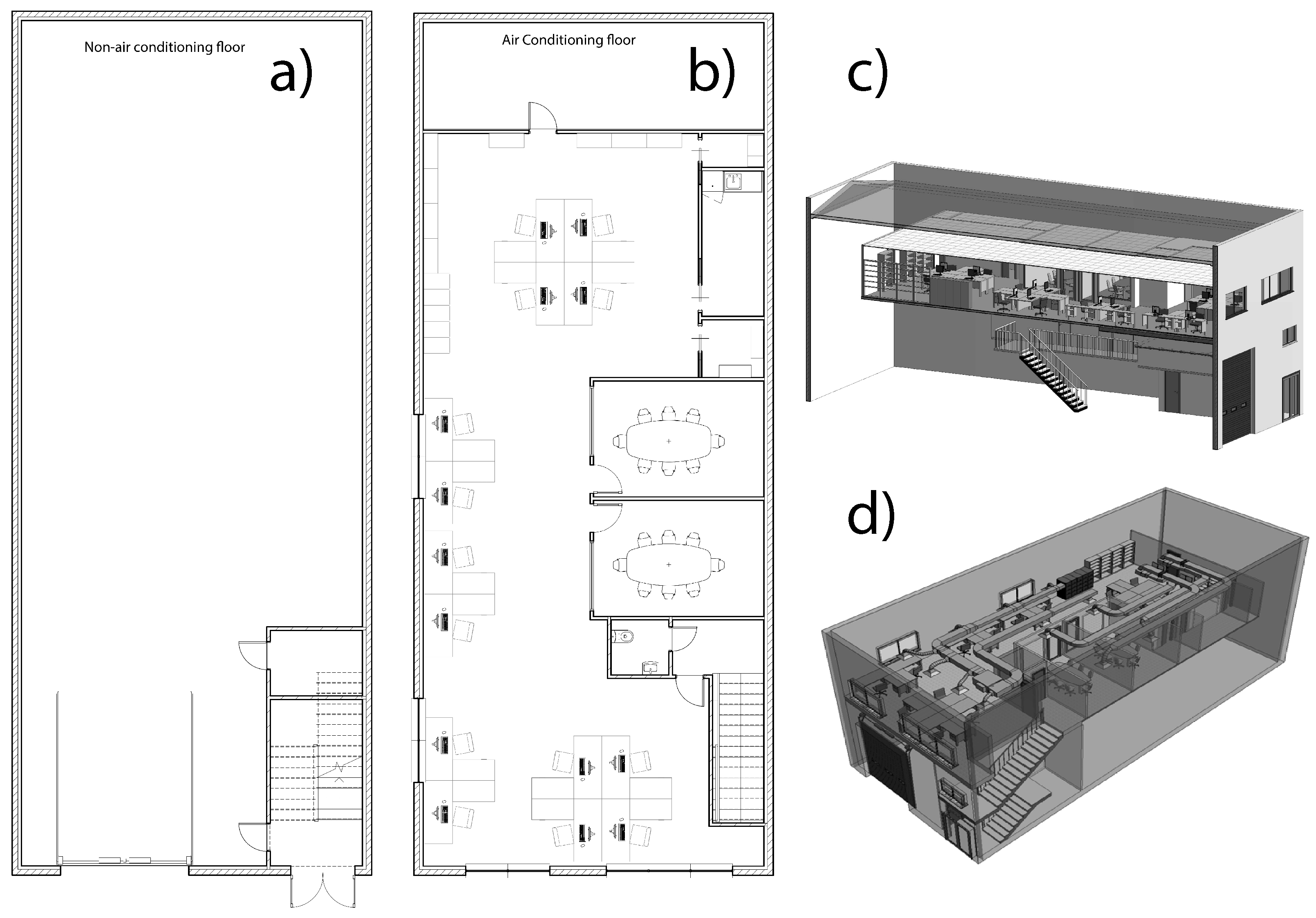
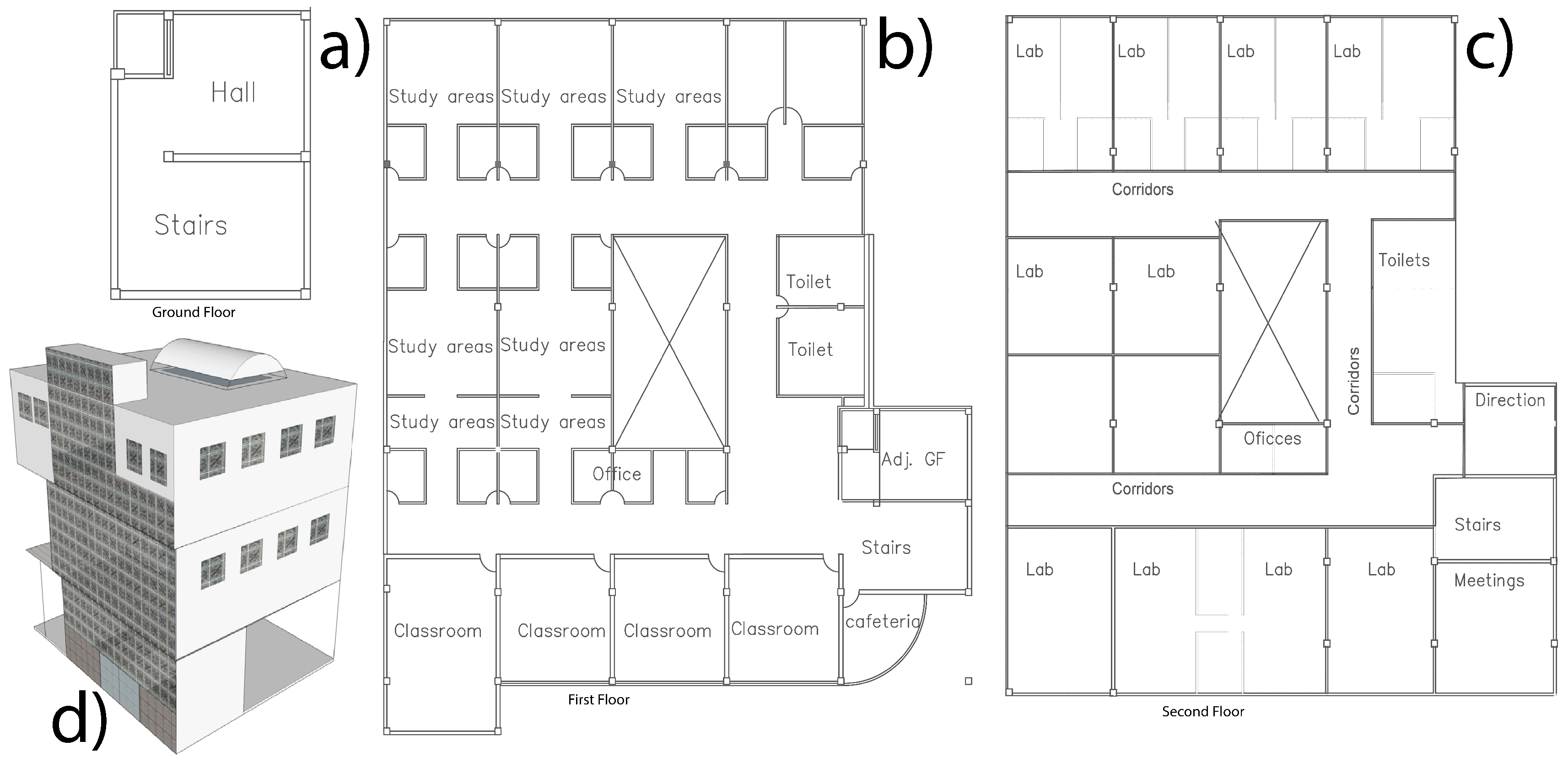
2.2. Building Structure And Use

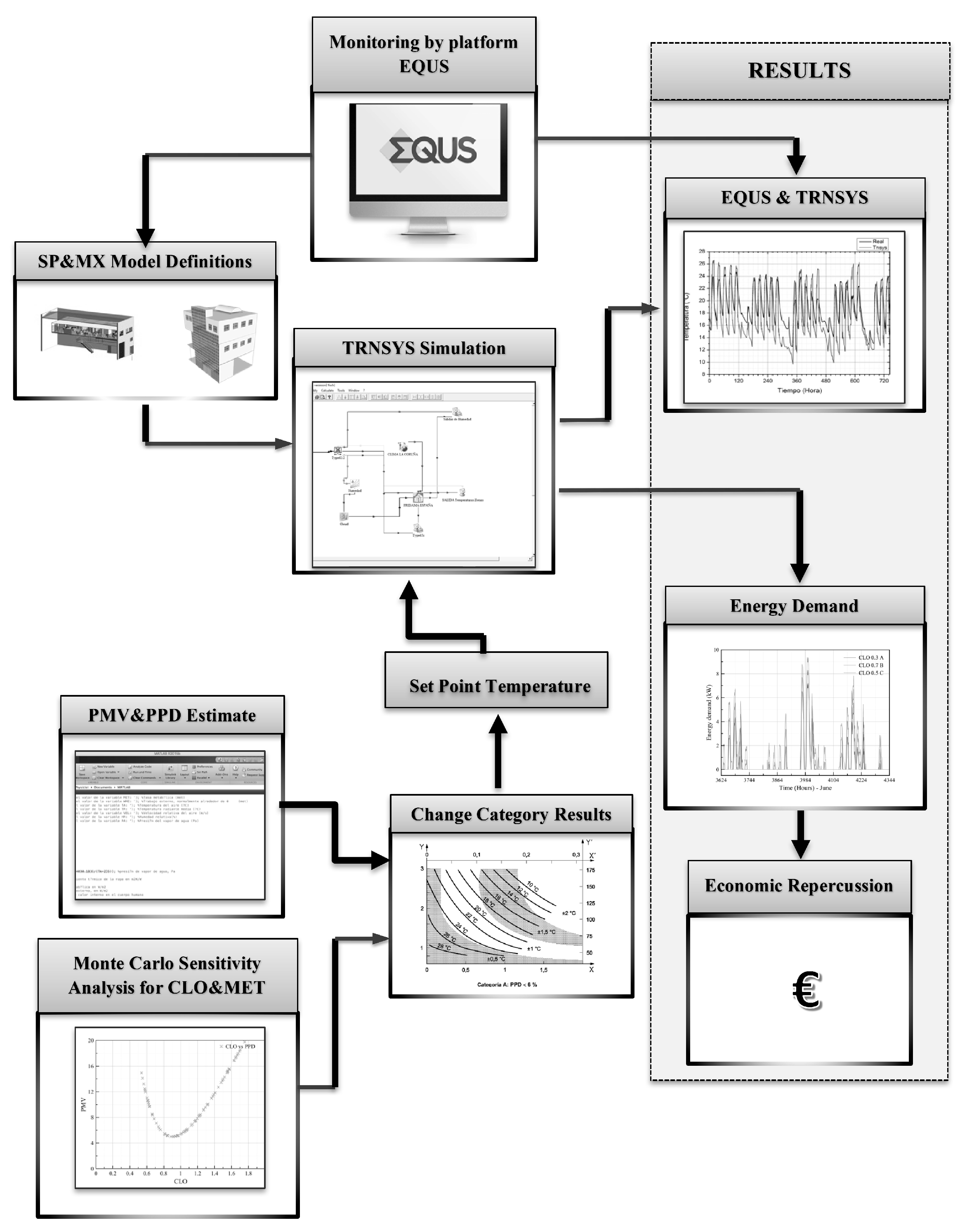
The base of the first building is of rectangular shape with an area of 218.14 m² (see Figure 1) and its main wall faces southwest (216° N). The building is distributed on two floors (defined as ground and first), being the lower level used for storage and the upper zone for offices, meeting rooms, and kitchen, among others uses. This building is the headquarters of a private company specialized in air-conditioning systems. The working hours, considered from Monday to Friday throughout the year, are from 08:30 a.m. to 06:00 p.m.

For the second case, the plant of the building has an “L” shape, covering an area of 1214 m² in each of its three heights that we define as: ground floor (GF), first floor (FF) and second floor (SF). The GF corresponds to a parking lot without vertical enclosures and a reception area, while the other two floors are classrooms, meeting rooms, laboratories, offices, etc. as is shown in Figure 2. The building hosts a research center on physics and mathematics (CICFIM), which is located behind of the School of Physics and Mathematics of the Universidad Autónoma de Nuevo León (Mexico). Its principal access is on the facade facing east, next to the campus stadium, to the west. This building starts the activities at 7:00 a.m., ending at 9:00 p.m. from Monday to Friday. Saturday’s schedule is from 10:00 a.m. to 2:00 p.m.

The building in Spain is made with three different types of envelopes: the vertical facing walls, the floor, and the roof. In

Table 1. Thermal and structural properties of adopted constructive solutions for case 1 (Spain).

Wall Types	Structure	Layer	t	κ	Cp	ρ	R
			(cm)	(kJ/mK)	(kJ/kgK)	(g/cm3)	(hm2K/kJ)
External Walls		Cement roughcast	1.5	5.040	1.10	2.00	--
		Concrete block	20	1.764	1.10	1.20	--
		Air chamber	5.0	--	--	--	0.05
		Plasterboard	20	0.900	1.00	0.90	--
U − value = 0.637 W/m2K
Floor		Ceramic Brick	25	4.104	0.90	1.25	--
		Compressed concrete	5.0	1.00	1.10	1.50	--
		Air chamber	0.4	0.612	1.40	1.20	--
U − value = 2.402 W/m2K
Roof		Galvanized Metal	2.5	180.1	1.50	7.85	--
		Air chamber	180	--	--	--	0.05
		Perlite ceiling	2.5	0.187	1.50	0.12	--
U − value = 0.934 W/m2K

we indicate that their respective thicknesses (t) are 46.5 cm, 30.4 cm and 185 cm. The building in Mexico

Table 2. Thermal and structural properties of adopted constructive solutions for case 2 (Mexico).

Wall Types	Structure	Layer	t	κ	Cp	ρ	R
			(cm)	(kJ/mK)	(kJ/kgK)	(g/cm3)	(hm2K/kJ)
Internal Walls		Plasterboard	1.5	0.900	1.00	0.90	--
		Mineral wool	6.0	0.130	1.03	0.05	--
		Plasterboard	1.5	0.900	1.00	0.90	--
U − value = 0.512 W/m2K
External Walls		Plasterboard Perforated brick Extruded polystyrene Air Chamber Hollow brick Cement mortar	1.0 9.0 5.0 5.0 14 1.0	1.080 2.736 0.122 -- 1.764 5.040	1.00 1.00 1.45 -- 0.92 1.05	0.80 1.60 0.03 -- 1.20 2.00	-- -- -- 0.05 -- --
U − value = 0.441 W/m2K
Floor & Roof		Concrete Cement mortar Extruded polystyrene Reinfor. concrete Pebble	3.0 1.0 6.0 15 15	4.140 5.040 0.122 8.280 2.916	1.00 1.05 1.45 1.00 0.92	1.80 2.00 0.03 2.30 1.70	-- -- -- -- --
U − value = 0.450 W/m2K
Divisions		Aluminum Mineral wool Aluminum	3.0 4.0 3.0	575 0.11 575	0.90 1.00 0.90	2.80 0.05 2.80	-- -- --
Divisions		Aluminum	3.0	575	0.90	2.80	--
		Mineral wool	4.0	0.11	1.00	0.05	--
		Aluminum	3.0	575	0.90	2.80	--
U − value = 3.296 W/m2K

has four types of envelopes: internal (9 cm) and external (35 cm) walls, as well as 10 cm-thick divisions. In this case, the same materials were used in the floor and the roof, with a total thickness of 40 cm.

In both Table 1 and Table 2, the physical characteristics of each layer of material are specified, such as thermal transmittance (U − value), thermal conductivity (κ), heat capacity ($C_p$), density (ρ) and resistance (R) in specific cases.

For both buildings, the properties of the windows are described in

Table A1. Thermal and structural properties in windows.

	Window Types	Glass	Thickness (mm)	% Frame	U (Wm−2K−1)	G-Value
Case 1 (Spain)	Type A	double low emissivity glass	4/6/4	15	3.44	0.76
Case 2 (Mexico)	Type 1	Single solar control glass	6	5	5.73	0.482
	Type 2	Single clear glass	6	15	5.73	0.837
	Type 3	Double clear glass	6/12/6	10	3.21	0.722
	Type 4	Single clear glass	6	35	5.73	0.837
	Type 5	Single clear glass	2	5	5.87	0.888
	Type 6	Single solar control glass	6	25	5.73	0.482

. In the first building (Spain) there are two types of zones, depending on whether there is air conditioning or not (see

Table A2. Distribution of the cases of study.

	Zones	Partitions	Characteristics
Case 1 (Spain)	Without air-conditioning (WAC)	Storage and air chamber of the roof.	Area (253.36 m2) Volume (1910 m3) Capacitance (2292.71 kJ/°K)
	Air-conditioned (AC)	2 Offices, 2 meeting rooms, small storage kitchen, rack, access and cleaning room.	Area (218.13 m2) Volume (610.78 m3) Capacitance (732.94 kJ/°K)
Case 2 (Mexico)	Zone GF-FF	GF: the reception of the building. FF: labs, offices, toilets, study areas, dining room.	Area (1142.68 m2) Volume (3366.99 m3) Capacitance (4040.39 kJ/°K)
	Zone SF	Labs, offices, toilets computer center, cleaning room, meeting room.	Area (1142.68 m2) Volume (3225.0 m3) Capacitance (3870.0 kJ/°K)
	Zone SL	Unused open space (Skylight)	Area (84.0 m2) Volume (462.0 m3) Capacitance (554.4 kJ/°K)

) in Appendix A. The second edifice (Mexico) is distributed in three partitions, because of the different uses and temperatures inside. Among its main characteristics are frame percentage, thermal transmittance (U) and solar gain (G − Value).

In Spain, the HVAC system consists on an inverter heat pump (2 × 1) and a split air–air unit, with a total refrigeration capacity of 17.2 kW, a heat power of 19.5 kW and an installed power of 6.5 kW. The diffusion of air is carried out by ducts and impulse/return grids. For the building in Mexico which a conventional technology, based on air-air heat pumps with 26 exterior units and indoor cassette units and a total cooling capacity of 349.4 kW. The heat output is 447.7 kW and the installed power is 166.4 kW.

3. Methodology

The main objective of this research is to show the consequences on the results of BIM-based simulations of subjective decisions made by the designers when using the environmental ergonomic standard ISO 7730 to calculate thermal comfort ranges and its impact on the energy demand of buildings, as well as its economic repercussion. The thermal sensation experienced by a human being is mainly due to the overall thermal balance of the body, which depends on the physical activity (met) and clothing (clo) of the subject, as well as by the environmental parameters: air temperature, radiant temperature, air speed, and air humidity [71]. We must stress that the definition of the parameters of human clothing and activity is done subjectively by the designer and therefore we refer to these quantities as Subjective Human Parameters (SHPs). The use of biometric data from wearable devices has been recently proposed as an interesting option for metabolic rate estimation in thermal comfort analysis [72].

The PMV and PPD indices, according to Fanger’s method [71] are commonly used to express warm and cool discomfort for the body as a whole, although thermal dissatisfaction may also be caused by unwanted heating or cooling of one particular part of the body (local discomfort). Therefore, when the previous factors are known, the thermal sensation for the occupants can be predicted, using a seven-point scale ranging from cold (−3) to hot (3), being 0 the value for “neutral sensation” [73]. The PMV may be computed from tables or may be measured by an instrument [74]. The methodology proposed in this paper consists of obtaining first the thermal performances of the buildings and then performing the SA for the SHPs used in the thermal comfort calculation, with the purpose of identifying which quantity has more influence on the BIM-based simulation outputs. Figure 3 shows a scheme of the procedure applied, consisting of the following steps, for both cases studied:

• Real-time tracking of the main variables using Equs web platform.
• TRNSYS modeling, getting the indoor temperature.
• Verification of the thermal simulation with measured temperature from Equs database.
• Mathematical estimation of PMV and PPD indices, according to ISO 7730.
• SA (Monte Carlo) to determine which parameter (activity and clothing) values yield significant variation on PMV and PPD outputs.
• New set-point temperatures are established, depending on the changes in the thermal categories in the previous step.
• TRNSYS recalculation of the energy demand for each set-point temperature from the Monte Carlo method.
• Evaluation of the variations in the energy demand for the different options.

3.1. Monitoring by Web Platform

A web platform for energy management of buildings named “Equs”, was developed with the purpose of control, maintenance and monitoring of energy consumptions and environmental variables as temperature, humidity and CO₂ levels. This tool also includes the possibility of remotely controlling any device by SCADA (Supervisory Control and Data Acquisition) system, ensuring the quality 6 of the statistical results. Equs collects in its database the information sent by the different sensors, allowing us to know the variation of the physical variables remotely, as access to these data can be obtained with any computer or other devices such as smartphones, which are connected to the Internet, making it very simple the treatment of the data, which can be done in the same device accessing to the values, in real time [69].

3.2. Trnsys Modeling of The Buildings

Through dynamic simulation tools, such as TRNSYS, we can define and evaluate the comfort and energy demand of the two buildings accurately; in both cases, we work with multi-zone building models. Notice that TRNSYS is integrated into two parts: TRNBuild, which reads and processes an input file, solving and plotting the system; and TRNSYS Studio, which is a library of components that can be used to model different systems. An advantage of using TRNSYS is the possibility to convert complex problems as multi-zone building models into smaller components, to allow the designer to establish the connections between the building and numerous other subsystems/components in the simulation environment [75].

To verify the energy demands of the structures, after analyzing the sensitivity with the Monte Carlo method of the set-point temperatures of the air-conditioning systems with the met and clo parameters, it has opted for its simulation in the program TRNSYS. To simulate the building, both in Spain and in Mexico, all the necessary inputs, dimensions, location, construction characteristics, etc. have been introduced into the program. This simulation will be verified later comparing the results that the TRNSYS throws in certain indoor temperature conditions, with the actual measurements of both the environmental conditions and the interior temperatures. Once the model is validated, we can calculate the variation of the energy demand in both buildings as indicated by the Monte Carlo SA to the parameters studied in ISO 7730.

Entering the buildings models in TRNSYS was done in two steps: first, in TRNBuild we implemented the different zones and all its elements as location, orientations, walls, layers of materials, gains, ventilation, infiltration, schedules, and comfort in TRNBuild. The second step corresponds to include in TRNSYS models as weather, inputs such as the building previously described and outputs that will show through graphics the thermal performance and energy demands of the buildings. Thus, first, we obtained the database of the buildings, which includes information such as orientations of the facades, materials for the walls and windows, the energy demand of the installed equipment, the working hours, the occupation, etc. The process of the definition of the buildings in TRNBuild includes the following information:

• Location and orientations. This information was described in Section 2.2
• Structure of the building: the materials detailed in Table 1, Table 2 and Table A1 were assigned from the software database.
• The zones described in Table A2, were created as WAC and AC for the first case, GF-FF, SF, and SL for the second case in the TRNBuild Manager.
• In

  Table A3. Types of schedules in the buildings.

  	Schedule Type		Hours	Use Factor
  Case 1 (Spain)	Daily	Daily 1	08:00 to 18:30	1
  		Daily 2	13:00 to 16:00	1
  		Daily 3	08:00 to 13:00	1
  			16:00 to 18:30	1
  	Weekly	Weekly 1	Monday to Friday	Daily 1
  		Weekly 2	Monday to Friday	Daily 2
  		Weekly 3	Monday to Friday	Daily 3
  Case 2 (Mexico)	Daily	Daily A	09:00 to 21:00	1
  		Daily B	07:00 to 21:00	1
  		Daily C	10:00 to 14:00	1
  	Weekly	Weekly A	Monday to Friday	Daily A
  			Saturday	Daily C
  		Weekly B	Monday to Sunday	Daily B

  we show the different types of schedules created for each building, we set a value of 1 in the periods where there is activity in the building, in any other case, including the weekend, the value is 0.
• In

  Table A4. Infiltrations and ventilation for each zone in summer and winter.

  Case of Study	Zones	Infiltrations Air Change per Hour		Ventilation Air Change per Hour
  		Summer	Winter
  Case 1: Spain	WAC	0.143	0.031	5.00
  	AC	0.066	0.067	1.65
  Case 2: Mexico	GF-FF	3.39	1.80	8.00
  	SF	3.41	1.81	8.00
  	SL	25.27	13.41	10.0

  we summarize the infiltrations for summer and winter in both cases. This information was calculated based on ASHRAE Standard 55.
• For calculating the ventilation we use standard EN 13779, ASHRAE 62 R. It was estimated a value for each zone which is shown in Table A2.
• The internal gains of the buildings are shown in

  Table 3. Input data of internal gains in the AC zone on Spain case.

  Gains	Description	Schedule	Total Energy Rate (W)
  Occupancy	15 Adults seated doing office work	Weekly 1	2250
  Computers	16 PC with monitor	Weekly 1	2240
  Artificial Artificial	37 fluorescent lamps in 218.12 m2	Weekly 1	3600
  Other	HVAC	Weekly 1	3332
  Gains
  	Coffee machine (10 cups)	Weekly 2	1500
  	Copy Machine (office type)	Weekly 3	1060
  	Microwave	Weekly 2	600
  	Refrigerator	All time	322
  	Plotter	Weekly 1	250
  	TV	Weekly 1	90

  and

  Table 4. Input data of internal gains in the different zones on Mexico case.

  Gains	Zones		Description	Schedule	Total Energy Rate (W)
  	GF-FF	SF			GF-FF	SF
  Occupancy	63	51	Adults seated doing office work	Weekly A	9450	7650
  Computers	54	50	PC with monitor	Weekly A	7650	7000
  Artificial	37	9	Fluorescent lamps (64 W)	Weekly A	2304	576
  Lighting	60	46	Fluorescent lamps (80 W)	Weekly A	4800	3680
  	64	62	Fluorescent lamps (40 W)	Weekly A	2560	2480
  Other			HVAC	Weekly B	21,320
  Gains	5	3	Coffee machine (10 cups)	Weekly A	1500
  	2	1	Water Cooler	Weekly B	1060
  	1	--	Microwave	Weekly A	600
  	2	1	Refrigerator	All time	322
  	10	12	Plotter	Weekly A	250
  	2	--	TV	Weekly A	90

  .
• The values of clothing factor, metabolic rate, relative air velocity were introduced in TRNSYS based on the ISO Standard 7730.

For estimation of comfort, it is important to note that thermal sensations are different between persons sharing the same environment. Perceptions of human beings about thermal comfort are very different because even people who stay in similar places have different opinions, because there exist many elements that impact the perception of human beings.

Thermal comfort is the main goal and has a strong influence in the thermal behavior of a building, for this reason, the values of clothing factor, metabolic rate, relative air velocity were introduced in TRNSYS, based on the ISO Standard 7730. In

Table 5. Input data of comfort in the two buildings, according to ISO 7730.

Parameters	Description	Value
Clothing factor	Summer 1: panties, t-shirt, shorts, thin socks, sandals	0.30 clo/0.050 m2K/W
	Summer 2: underpants, t-shirt, light pants, thin socks, shoes	0.50 clo/0.080 m2K/W
	Summer 3: underwear, shirt, pants, socks, shoes	0.70 clo/0.110 m2K/W
	Winter: underwear, shirt, pants, thermal jacket, socks, shoes	1.20 clo/0.185 m2K/W
Metabolic Rate	Rest, seated	1.0 met/58 W/m2
	Seated, light work (office, home, school, laboratory)	1.2 met/70 W/m2
External Work	In general, the external work is around 0	0 met
Relative air velocity	The air velocity relative to the person	0.3 m/s

, we show the numbers for both cases in summer and winter. We decided to set the same values of clothing and activity, because the characteristics of the occupants are very similar. It should be noted that these values are subjective decisions on the part of the designer. The analysis of the impact of these decisions is one of the main goals of this work.

4. Simulation of Building Models

In this section, it is presented the dynamic thermal simulation model in TRNSYS Studio of the building previously described in TRNBuild, for this purpose we use multi-zone building model “TYPE 56” that can be connected to a large number of other components, including weather data, HVAC systems, occupancy schedules, controllers, output functions, etc. Other models used were Type 62, Type 109-TMY2, and Type 65.

Under ISO Standard 7730, the evaluation of the levels of comfort was calculated using a mathematical MATLAB software package for the interactive numerical study of dynamical systems. The change of PMV and PPD in base of its parameters such as metabolic rate, clothing insulation, and air temperature, is easier of visualizing in MATLAB than in TRNSYS because you can modify its parameters independently and realize studies more specific such SA.

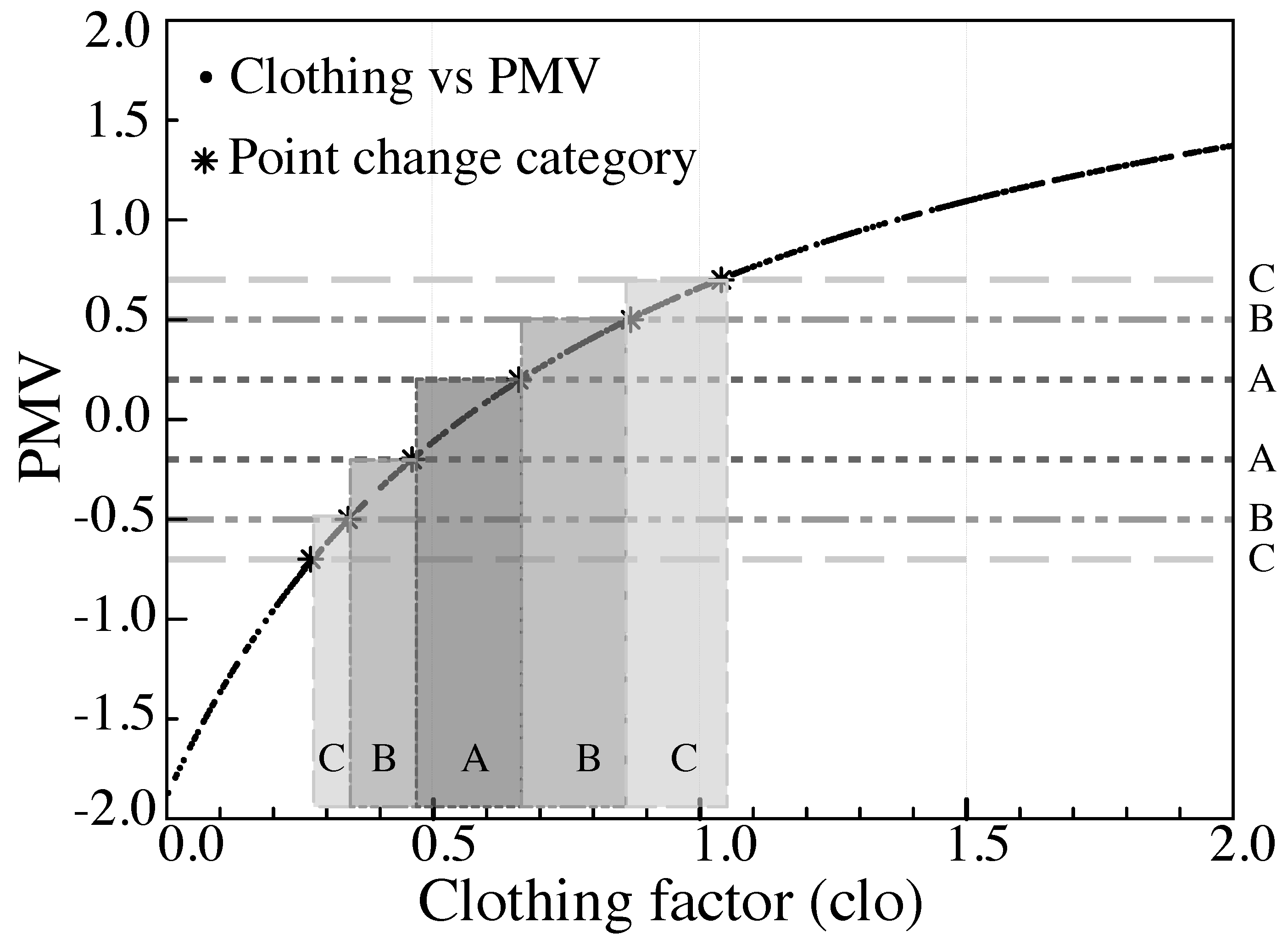
Monte Carlo Sensitivity Analysis

The principal aim of the SA using a Monte Carlo code is to obtain the variation of the PPD and PMV concerning the possible choices of the clo and met that are indicated in the annexes of the 7730 for thermal comfort calculations. In this way, by changing the values of clo and met according to what is reported in the tables of ISO 7730, we try to find out how the environmental category varies and, consequently, the set-point temperature. The SA is extensively suitable for associating input parameters with the overall building performance (for example, the temperature or demand for heating or cooling) [64]. The individual contribution from specific input can be determined by SA to prepare for future optimization of energy, climate, and economic performance [76,77]. SA methods can typically be classified to the local SA where input parameters are varied one at a time and the global SA where all inputs are changed simultaneously.

Sampling-based methods for uncertainty and SA have become very popular. The sampling-based Monte Carlo method is a procedure that performs a model repeated times with random samples generated from input distributions. It provides approximate solutions to both uncertainty and sensitivity analyses by making statistical modeling investigations [78]. The method can manage complex black box models irrespective of the linearity and continuity, and generate a probability distribution for each output depending on input distribution types [62].

The analysis under consideration can be represented by a function $y\left(x\right)$ where:

$$\mathbf{y}\left(x\right)=[y_1\left(x\right),y_2\left(x\right),\dots ,y_{n_Y}\left(x\right)]$$

(1)

and

$$\mathbf{x}=[x_1,x_2,\dots ,x_{n_X}]$$

(2)

designates the outputs and inputs of the analysis, respectively. Successively, sensitivity in x results in a corresponding sensitivity in $y\left(x\right)$. Furthermore, the distributions

$$\mathbf{D}=[D_1,D_2,\dots ,D_{n_X}]$$

(3)

must be well-defined to characterize the uncertainty associated with the elements of x, where $D_i$ is the distribution associated with $x_i$ for $i=1,2\dots n_X$.

The most common way for applying SA in building performance analysis consists on the following steps: determine input variations, create building energy models, run energy models, collect simulation results, run SA and presentation of SA results [64]. Determining the probability distributions of input parameters is the first step in any SA, which depends on the election of sensitivity method. In the present study, Monte Carlo SA is used, considering N input parameters defining the system:

$$O_i(P_1,P_2,\dots P_N)i=1,2,\dots ,M.$$

(4)

Suppose that the parameter $P_j$ can change within a range given by $\Delta P_j$. To analyze the influence of the parameter $P_j$ in the objective $O_i$, we proceed first generating a uniform random number distribution $r\in [0,1]$, thus:

$$P_j^1=(P_j-\Delta P_j)+2r\Delta P_j,P_j^1\in [P_j-\Delta P_j,P_j+\Delta P_j],$$

(5)

gives us the first random value $P_j^1$. With the value of N randomly generated parameters $P_j^1(j=1,2,\cdots ,N)$, we obtain a value of $O_i^1$, which is the first evaluation of the objective $O_i$. We repeat this procedure up to the desired number of random evaluations. We can randomly change each one of the parameters or we can apply random variations to one of the parameters keeping constant the value of the rest.

For this work, the objectives $O_i$ are the PMV and PPD indices, which are a function of different parameters mentioned in the previous sections. To analyze the influence on the thermal performance of the buildings, the $P_j$ parameters are CLO and MET. Depending on the admissible ranges for PMV and PPD, three kinds of comfort zones or categories of thermal requirements are defined by UNE-EN ISO 7730 as: category I (or class A) (PPD < 6 %, i.e., −0.2 < PMV < 0.2), category II (or class B) (PPD < 10%, i.e., −0.5 < PMV < 0.5) and category III (or class C) (PPD < 15%, i.e., −0.7 < PMV < 0.7). The ranges of recommended air temperatures for different types of buildings depending on the previous categories are shown in

Table 6. The range of recommended air temperatures for offices and classrooms, according to ISO 7730.

Type of Building	Activity (W/m2)	Category	Temperature (°C)
			Summer	Winter
Classrooms Main Hall Offices Conferences room	70	A B C	24.5 ± 1.0 24.5 ± 1.5 24.5 ± 2.5	22.0 ± 1.0 22.0 ± 2.0 22.0 ± 3.0

[26]. Based on the results of the SA, we can establish the set-point temperature for the cooling and heating seasons.

We use the SA based on the Monte Carlo method, randomly generating a uniform distribution for clo from 0 to 2 and met from 0.8 to 4, since in this range the PMV index lies between −2 and +2, taking into account that this is the range suggested by the standard. A uniform distribution corresponds to the case of a random variable that can only have values between two extremes a and b, so that all the intervals of the same length (within (a, b)) have the equal probability.

The above definition shows that the density function must be the same value for all points within the interval (a, b) (and zero outside the range), i.e.,

$$f_X\left(\chi \right)=\left\{{\displaystyle \frac{1}{b-a}}si\chi \in (a,b)y0si\chi \notin (a,b)\right\}$$

(6)

The results of the SA on the comfort index (PMV and PPD) for the clothing and metabolic rate are shown in Figure 4 and Figure 5, respectively. The thermal category changes according to PMV and PPD values, which in turn depend on the subjective decisions of clo and met. Figure 4 shows that for category A, the clo values vary from 0.46 to 0.66, for B of 0.34 to 0.46 clo and 0.66 to 0.87 clo. Category C is between 0.27 to 0.34 clo and 0.87 to 1.04 clo. For the case of met and PPD, in Figure 5 we show that category A lies between met values from 0.83 to 1.04. For the case of category B, it remains from 0.8 to 0.83 met and 1.04 to 1.16 clo. Finally, category C corresponds to the range from 1.16 to 1.31 met.

An attractive alternative in this type of SA, it is to use a normal distribution, which is one of the theoretical distributions best studied in statistical texts and more in practice, also called Gaussian distribution. Its importance is mainly due to the frequency with the variables other than natural and everyday phenomena, approximately, this distribution.

The normal distribution is determined by two parameters, their mean and their standard deviation, usually denoted by μ y σ [79]. With this notation, the density of the distribution Gaussian is given by the equation:

$$f\left(x\right)=\frac{1}{\sigma \sqrt{2\pi }}exp\left\{\frac{-1}{2}{\left(\frac{x-\mu }{\sigma }\right)}^2\right\};-\infty <x<\infty$$

(7)

For the case of a normal distribution, we have randomly generated values for clo with μ = 1.0, setting the metabolic factor to 1.2 met and, varying the standard deviation ${\sigma }_{clo}=0.025,0.05,0.075,0.1$ and 0.125. For these values, we obtain the distribution of the PMV and PPD values and, by adjusting to a normal distribution, we obtain the values of μ and σ for the PMV and PPD. Similarly, for the case of the met (metabolic factor) a $\mu =1.2$ has been established, setting the clothing factor to 1.0 clo and varying the standard deviation ${\sigma }_{met}=0.025,0.05,0.075,0.1$ and 0.125.

That is to say, we see easily as variations in the values of clo and met, they are transferred through the model to variations of PMV and PPD, and therefore, we can see the sensitivity of the model to these variations of the clo and met parameters.

That is, we have obtained the relation of the variations of the clothing (clo) and activity (met) with the widths (σ) of the PMV and PPD, with the objective of observe which of the two parameters that the designer enters in a subjective manner, produces a more significant impact on the output of the model.

In the Figure 6a, the relationship between the widths of the distributions of clo and met and the value of σ_PMV is presented. For example, for a width of 5 % with respect to the central value of clo $\mu =1$ and (${\sigma }_{clo}=0.10$), a value of σ_PMV of 0.150 is obtained and for a width of 5 % with respect to the central value $\mu =1.2$ of met (${\sigma }_{met}=0.10$), a value of σ_PMV of 0.184 is obtained. Therefore, the impact of the metabolic factor (met) is higher than that of the clothing factor (clo) for the PMV case.

In the same way, for each percentage of variation in the values of clo and met we have a value of σ_PPD, which is shown in the Figure 6b, for example: for a width of 12.5 % the value of σ_PPD is 1.990 for a variation in clo and 2.594 if the parameter met varies. Also, the values predict that the impact of the metabolic factor (met) is greater than the clothing factor (clo) in the PPD.

5. Results

In this section, we discuss the results of the simulations of both buildings. First, we will show the verification of the monitoring using the data from Equs and the TRNSYS simulation of each building. Then, after a second simulation, we will get the energy demand using the calculated results for the category change, depending on the estimation of the PMV and PPD values as well as the sensitivity analysis of the CLO and MET variables. Finally, we analyze the economic impact of energy demand savings.

As noted before, this work joins BIM-based energy simulations and SA of two non-residential buildings in two seasons (summer and winter) under the international standard ISO 7730. This norm has been studied in previous papers from different perspectives: the effect of personal factors in comfort assessment [80], energy simulation [27], thermal comfort in outdoor urban spaces [81] or the validity of ISO-PMV for predicting comfort votes in everyday thermal environments [82], among others. However, to our knowledge, the effect on the energy demand of the diversity of possibilities offered by ISO 7730 for the choice of clo and met results, depending on the values chosen by the designer, was not previously calculated.

5.1. Real-Time Monitoring and Validation of The Models

Real-time tracking made online with Equs demonstrates the reliability of the measurements that validate the computational simulations. In Figure 7 we show the temperatures measured from 1 January to 31 October 2015 of the air-conditioning zone of the building in Spain, located 43°18′ north and 8°17′ west. In the first month (January, winter season) the lowest temperature of the period is 12.53 °C registered on Saturday 17. The highest temperature (30.48 °C), was achieved on Monday, 15 June (summer). The mean temperature was 22.43 °C. For the study of the outside temperature, we observe that the cold and hot temperatures are between 2 °C and 41 °C, approximately. The mean temperature outside the building was 15.49 °C.

The comparison between the real data and the simulations is required to have reliable simulations of the buildings. Currently, a simulation of a building’s energy consumption is usually considered “calibrated” if the criteria set out by ASHRAE Guideline 14 is met [83]. Accordingly, the model can be considered “calibrated,” according to current international criteria to accept BES models, provided that considerable accordance is reached between the measured and simulated data [84]. We must stress that there is no unique model that meets the previous criteria and therefore, several alternative models of the same building can be considered to be “calibrated”. Moreover, it should be noted that our calibration is very accurate for the simulated environment (e.g., temperature profiles). As an example, the parallelism among experimental data and the modeling for internal air temperature for the month of June from the hour 3624 to 4344, is shown in Figure 8a. For the period of June, the maximum difference between the simulated and measured temperatures is 1.47 °C, being the mean deviation 0.49 °C. These values have no influence with respect to indoor comfort, showing that the results of our model are basically correct.

In Figure 8b we show the temperature of a single day of June (24 h from hour 3914 to 3938 of the simulation). We can observe in more detail the difference between the calculated and the measured temperature for the period, where the minimum variation is of 0.04 °C (obtained in working hours) and the mean difference is of 0.35 °C. The maximum variation is 0.72 °C. These results were obtained within the situation described in the previous sections. In particular, during the occupancy periods, the metabolic rate (met) of the occupiers was selected as to be “seated light work”, which corresponds to 70 W/m² or 1.2 met. The clothing factor (clo) was established to 0.7 for the summer period and 1.2 for winter. Notice that a clothing with factor 1.2 clo corresponds to: underwear, shirt, pants, thermal jacket, socks, shoes. Summer clothing of 0.7 clo corresponds to underwear, shirt, pants, socks, shoes [26]. Table 5 shows the input that was used for the simulation for the base case scenario. In Figure 9 we can observe the energy demand in the initial configuration, where the set point was established in 23.8 °C.

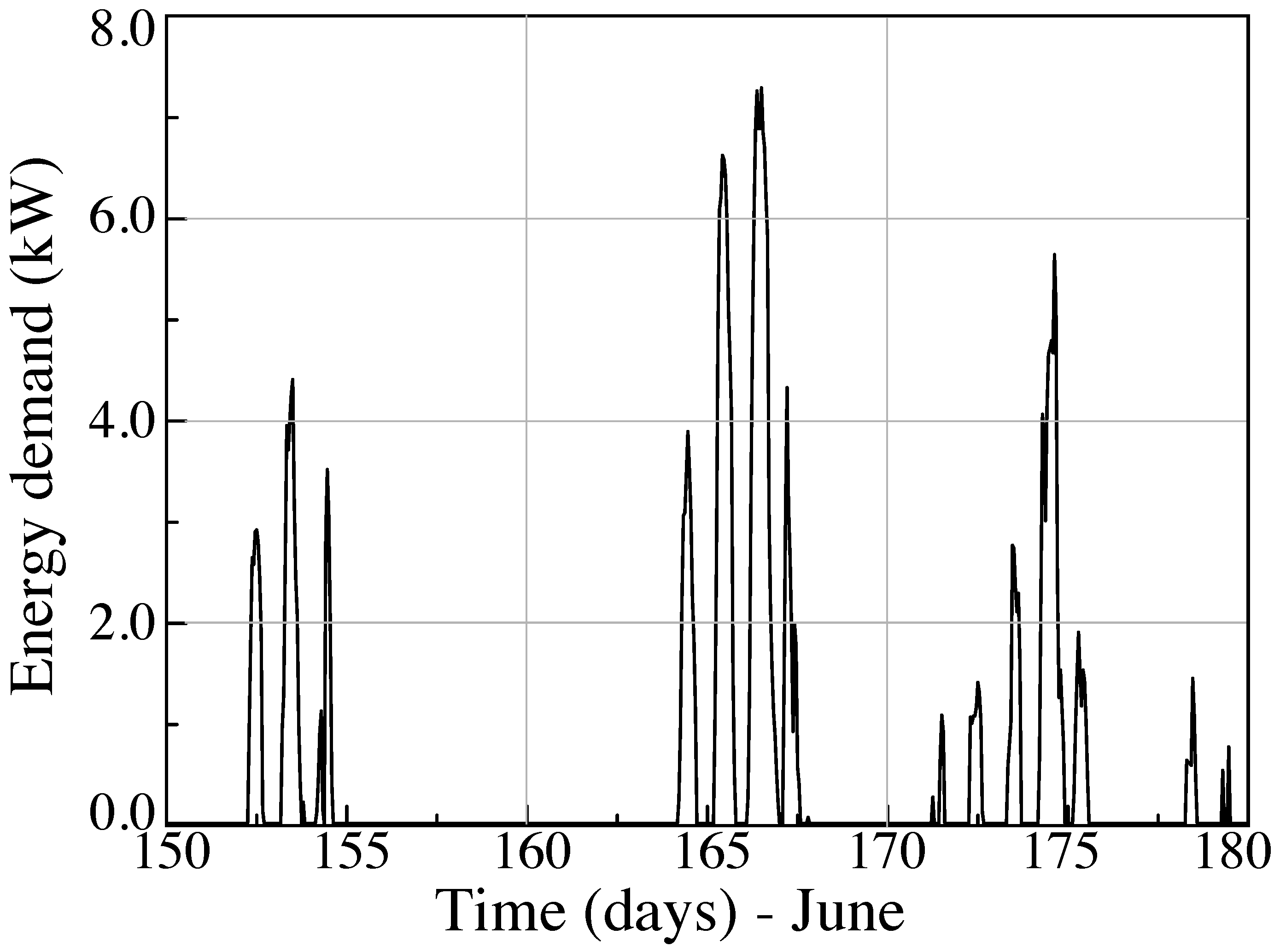
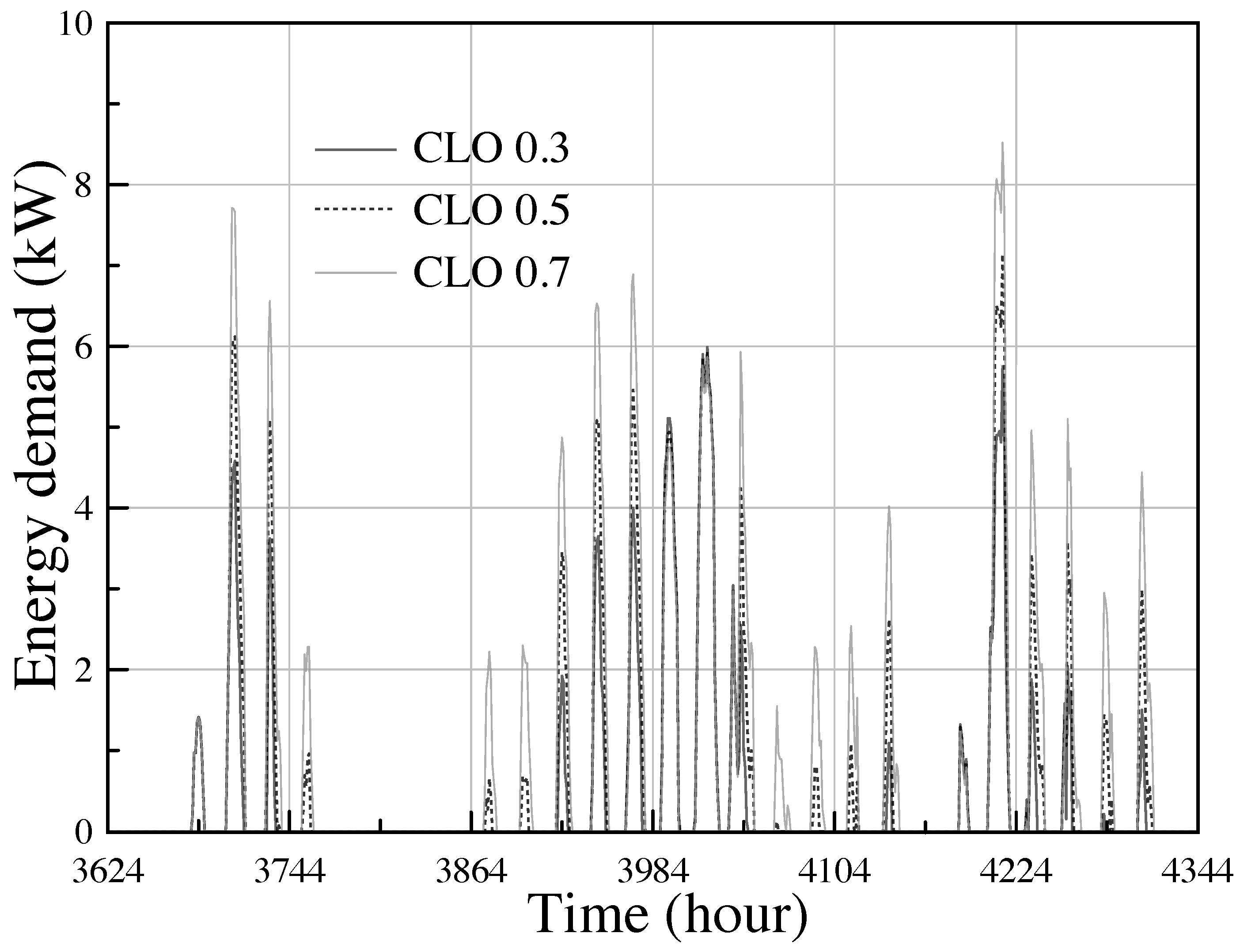
5.2. Evaluation of the Variations in the Energy Demand

The main goal of the application of a SA in this work is to visualize in a simpler and more detailed way than in TRNSYS, the impact of subjective decisions made by the designer on the values of insulation of clothes and activity for thermal comfort, which are defined in the TRNSYS simulation program. Based on ISO 7730, the insulation of clothes (clo) can be estimated directly from the combination of clothes or by adding the partial insulation values for each clothes. For example, typical value of clothes insulation for summer (cooling) and winter (heating) are 0.5 and 1 clo, respectively. Therefore, these quantities can be determinant for the different types of clothes that the occupants use and thus, the designers have a greater margin of error when determining by subjective decisions the values of clothing parameters.

Once we have made the variation of clo and met, we obtain variations in the PMV and PPD indices, these values of the indices allow us to define the thermal category based on the definition of the ISO 7730 standard. This category establishes the range of recommended temperatures for these input parameters of comfort. In this permissible temperature range, we can select a value of set-point temperature, to introduce it to our validated BIM model and thus obtain the new energy demand.

For instance: summer light clothing insulation of 0.5 clo includes items such as underpants, short–sleeved shirt, light pants, thin socks, or shoes. In our case, we choose for both cases of study a mean value of 0.7 clo that includes underwear, shirt, pants, socks, shoes, which are also considered light clothing for the same season in this type of buildings. Analogously, the estimation of the value of activity or metabolic rate (met), which represents a heat production depending on the activity level, also depends on the subjective decision made by the designer. According to ISO 7730 for an activity corresponding to this type of buildings such as office, school, and laboratory, the activity parameter can vary from 1.0 to 1.6 met. For this work we assumed a value of 1.2 met for the energy simulations on TRNSYS.

Thus, it is of fundamental importance to determine the impact of the mentioned subjective choices of clothing and metabolic factor, on the values of the PMV and PPD indexes, which show the level of thermal comfort and local thermal comfort criteria, reporting the environmental requirements that are considered acceptable for global thermal comfort, including the local discomfort.

We must notice that a variation in the clo values of summer clothing, from 0.3 to 0.8, causes a change in category from A to C. In Figure 10, the impact on the calculation of energy demand is clearly shown that has the change of environmental category.

According to the SA results and the results of Table 6, we established in TRNSYS the new values for clo and set-point temperature. The first configuration was set for a value of clo of 0.7 with a set-point temperature of 23.5 °C, which belongs to category A. For category B, we used a temperature of 24 °C and clo of 0.5. This configuration was initially defined for the validation of the TRNSYS simulation previously shown. Finally, a set-point temperature of 25 °C for category C and clo of 0.3 was considered. As an example, for the month of June, from Figure 10 for clo values of 0.3, 0.5 and 0.7, we obtain a total energy demand of 347.19 kW, 565.05 kW, and 885.2 kW, respectively.

In

Table 7. Cumulated energy demand between June and September, with varying values of clo and met, for different set temperatures based on the categories of thermal comfort.

Category (Case)	Set Temp	Cumulated Energy Demand (kWh/m2) for clo & met (June to September)
		0.3 clo	0.5 clo	0.7 clo	0.8 met	1.0 met	1.2 met
A (Spain)	23 °C	46.01	46.32	46.51	48.02	48.20	48.85
B (Spain)	24 °C	44.67	44.69	44.91	46.61	46.72	46.84
C (Spain)	25 °C	43.86	43.93	43.99	45.84	45.89	45.95
A (Mexico)	23 °C	119.53	120.76	122.03	150.35	152.85	155.36
B (Mexico)	24 °C	108.42	109.42	110.44	126.43	128.71	131.02
C (Mexico)	25 °C	99.67	100.44	101.23	106.09	106.85	108.93

it can be observed that changes in the energy demand due to variations in the designer’s criteria in climates such as Mexico, can reach up to 22% depending on the choice of clo and up to 23% in energy demand, depending on the choice of the activity rate made by the designer. As it can be seen after the analysis of the Monte Carlo method, the BIM calculation is very sensitive to both the appropriate choice of the met and the clo choice. In the case of the clo we have studied variations of daily clothing in summer with clo 0.3 (panties, t-shirt, shorts, thin socks, sandals), clo 0.5 (underpants, t-shirt, light pants, thin socks, shoes), clo 0.7 (underwear, shirt, pants, socks, shoes).

All previous values of clo are assignable to the attire of the occupants of both buildings studied both in the case of Spain and in Mexico, in summer. However, after analyzing it by the Monte Carlo method and calculating the environmental category by the TRNSYS program, we see that in both buildings for a room 0.3 the comfort in the buildings studied is in the category A ranges; for a clo of 0.5 in category B and if the clo is 0.3, in category C (Figure 4). This variation in the category, due to the uncertainty in the choice of the clo on the part of the designer, can have, consequently, alterations in the energy demand.

As it can be appreciated from the values of Table 7 the change is more than 20%, for the building in Mexico. For the building in Spain, the variation in the calculation of the energy demand, despite having a higher sensitivity, is much lower (only 6%). This discrepancy is due to the different volumes of the two buildings. The higher the volume, the greater the energy demand and therefore the variations of the environmental categories that determine the thermal comfort inside have a much greater impact.

With respect to the met, according to ISO 7730, the cases of a technical office (main activity of the building of Spain) and a University (main activity of the building of Mexico) correspond to met 1 (sitting rest), and met 1.2 (office activity, school, home, laboratory). As it can be appreciated from the values of Table 7, the higher variations in the calculation of energy demand in buildings have been again in the case of Mexico (more than 20%). In the case of the building in Spain the oscillation is only of 6.6%.

6. Conclusions

In the present work, we have analyzed, within the mandatory standard ISO 7730, the influence of the designer’s choice of values for human metabolic index and insulation by clothing that can be selected for the estimation of the energy demand of structures. We have demonstrated that the diversity of possibilities offered by ISO 7730 for the choice of clo and met results in significant differences in indoor comfort conditions, leading to non-negligible changes in the calculations of energy consumption.

It has been clearly outlined that the higher the cooling demands, the greater the sensitivity, generating greater differences according to the designer’s choice. Since ISO 7730 is an international norm, given the great variety of existing climates, it is vital to take into account this peculiarity of the system at the time of its application and in the choice of the designer, who must be familiar with the procedure. The international norm ISO 7730 is a reference in most of the countries of the world and nevertheless requires of an experienced designer for an appropriate application. Therefore, we have shown in the present work the considerable impact of the designer’s subjective choices on the calculation of the energy demand of buildings, as well as the extra costs cumulated, depending on the election of the amounts of activity or clothing, based on the environmental ergonomic standard ISO 7730. We consider that our SA of the parameters mentioned above using the Monte Carlo method will help to define the most appropriate metrics to be admitted, depending on the aim and type of the modeling performed.

We have calculated that the effect of to the different possibilities of election within the ISO 7730 can reach a quarter of the energy demand, showing that this standard is susceptible to the designer’s choice of the clo and met. As the ISO 7730 is the only standard which applies to the building regulations in many parts of the world, we conclude that the norm could be revisited from the perspective of energy efficiency, maybe including recommendations from other standards such as EN 15251-2007 or ISO 17772-1-2017, designed explicitly for providing environmental input parameters for design and assessment of energy performance of buildings.

References

1. Hemsath, T.L.; Bandhosseini, K.A. Sensitivity analysis evaluating basic building geometry’s effect on energy use. Renew. Energy 2015, 76, 526–538. [Google Scholar] [CrossRef]
2. Griego, D.; Krarti, M.; Hernandez-Guerrero, A. Energy efficiency optimization of new and existing office buildings in Guanajuato, Mexico. Sustain. Cities Soc. 2015, 17, 132–140. [Google Scholar] [CrossRef]
3. Lin, H.W.; Hong, T. On variations of space-heating energy use in office buildings. Appl. Energy 2013, 111, 515–528. [Google Scholar] [CrossRef] [Green Version]
4. Pikas, E.; Thalfeldt, M.; Kurnitski, J. Cost optimal and nearly zero energy building solutions for office buildings. Energy Build. 2014, 74, 30–42. [Google Scholar] [CrossRef]
5. Terés-Zubiaga, J.; Campos-Celador, A.; González-Pino, I.; Escudero-Revilla, C. Energy and economic assessment of the envelope retrofitting in residential buildings in Northern Spain. Energy Build. 2015, 86, 194–202. [Google Scholar] [CrossRef]
6. Lee, J.; Kim, J.; Song, D.; Kim, J.; Jang, C. Impact of external insulation and internal thermal density upon energy consumption of buildings in a temperate climate with four distinct seasons. Renew. Sustain. Energy Rev. 2017, 75, 1081–1088. [Google Scholar] [CrossRef]
7. IEA. World Energy Outlook 2017; Organisation for Economic Co-Operation and Development, OECD: Paris, France, 2017. [Google Scholar]
8. Anderson, J.E.; Wulfhorst, G.; Lang, W. Energy analysis of the built environment—A review and outlook. Renew. Sustain. Energy Rev. 2015, 44, 149–158. [Google Scholar] [CrossRef]
9. Abdelaziz, E.; Saidur, R.; Mekhilef, S. A review on energy saving strategies in industrial sector. Renew. Sustain. Energy Rev. 2011, 15, 150–168. [Google Scholar] [CrossRef]
10. Nejat, P.; Jomehzadeh, F.; Taheri, M.M.; Gohari, M.; Majid, M.Z.A. A global review of energy consumption, CO2 emissions and policy in the residential sector (with an overview of the top ten CO2 emitting countries). Renew. Sustain. Energy Rev. 2015, 43, 843–862. [Google Scholar] [CrossRef]
11. Balaras, C.A.; Droutsa, K.; Dascalaki, E.; Kontoyiannidis, S. Heating energy consumption and resulting environmental impact of European apartment buildings. Energy Build. 2005, 37, 429–442. [Google Scholar] [CrossRef]
12. Pérez-Lombard, L.; Ortiz, J.; Pout, C. A review on buildings energy consumption information. Energy Build. 2008, 40, 394–398. [Google Scholar] [CrossRef]
13. Galvin, R. Thermal upgrades of existing homes in Germany: The building code, subsidies, and economic efficiency. Energy Build. 2010, 42, 834–844. [Google Scholar] [CrossRef] [Green Version]
14. Creyts, J.C. Reducing US Greenhouse Gas Emissions: How Much at What Cost?: US Greenhouse Gas Abatement Mapping Initiative. McKinsey & Co. 2007. Available online: https://www.mckinsey.com/business-functions/sustainability/our-insights/reducing-us-greenhouse-gas-emissions (accessed on 1 March 2018).
15. Chappells, H.; Shove, E. Debating the future of comfort: Environmental sustainability, energy consumption and the indoor environment. Build. Res. Inf. 2005, 33, 32–40. [Google Scholar] [CrossRef]
16. Geva, A.; Saaroni, H.; Morris, J. Measurements and simulations of thermal comfort: A synagogue in Tel Aviv, Israel. J. Build. Perform. Simul. 2014, 7, 233–250. [Google Scholar] [CrossRef]
17. Nguyen, A.T.; Reiter, S. Passive designs and strategies for low-cost housing using simulation-based optimization and different thermal comfort criteria. J. Build. Perform. Simul. 2014, 7, 68–81. [Google Scholar] [CrossRef]
18. Rey Martínez, F.J.; Chicote, M.A.; Peñalver, A.V.; Gónzalez, A.T.; Gómez, E.V. Indoor air quality and thermal comfort evaluation in a Spanish modern low-energy office with thermally activated building systems. Sci. Technol. Built Environ. 2015, 21, 1091–1099. [Google Scholar] [CrossRef]
19. Wardiningsih, W.; Troynikov, O. Force attenuation capacity and thermophysiological wear comfort of vertically lapped nonwoven fabric. J. Text. Inst. 2017, 109, 1–9. [Google Scholar] [CrossRef]
20. Ashrae, A.S. Standard 62-1989, Ventilation for Acceptable Indoor Air Quality, Atlanta, GA; American Society of Heating, Refrigerating, and Air Conditioning Engineers, Inc.: New York, NY, USA, 1989. [Google Scholar]
21. MacArthur, J.; Arens, E.; Gonzalez, R.; Berglund, L.; Spain, S.; Madsen, T.; Oleson, B.; Reid, K. HVAC is for people. Ashrae Trans. 1986, 92, 5–64. [Google Scholar]
22. Oropeza-Perez, I.; Petzold-Rodriguez, A.H.; Bonilla-Lopez, C. Adaptive thermal comfort in the main Mexican climate conditions with and without passive cooling. Energy Build. 2017, 145, 251–258. [Google Scholar] [CrossRef]
23. Standard 55 Thermal Environmental Conditions For Human Occupancy; ASHRAE: New York, NY, USA, 2010.
24. CEN. 15251-Criteria for the Indoor Environment, Including Thermal, Indoor Air Quality (Ventilation), Light And Noise, 2006; CEN: Brussels, Belgium, 2006. [Google Scholar]
25. Matzarakis, A.; Mayer, H.; Iziomon, M.G. Applications of a universal thermal index: Physiological equivalent temperature. Int. J. Biometeorol. 1999, 43, 76–84. [Google Scholar] [CrossRef]
26. Standard 7730. Ergonomics of the Thermal Environment—Analytical Determination and Interpretation of Thermal Comfort Using Calculation of the Pmv and Ppd Indices and Local Thermal Comfort Criteria; International Organization for Standardization: Geneva, Switzerland, 2005.
27. Peeters, L.; De Dear, R.; Hensen, J.; D’haeseleer, W. Thermal comfort in residential buildings: Comfort values and scales for building energy simulation. Appl. Energy 2009, 86, 772–780. [Google Scholar] [CrossRef] [Green Version]
28. Ahmed, K.; Akhondzada, A.; Kurnitski, J.; Olesen, B. Occupancy schedules for energy simulation in new prEN16798-1 and ISO/FDIS 17772-1 standards. Sustain. Cities Soc. 2017, 35, 134–144. [Google Scholar] [CrossRef]
29. Antoniadou, P.; Papadopoulos, A.M. Occupants’ thermal comfort: State of the art and the prospects of personalized assessment in office buildings. Energy Build. 2017, 153, 136–149. [Google Scholar] [CrossRef]
30. Oropeza-Perez, I.; Østergaard, P.A. Potential of natural ventilation in temperate countries—A case study of Denmark. Appl. Energy 2014, 114, 520–530. [Google Scholar] [CrossRef]
31. Zhang, L.; Zhang, L.; Wang, Y. Shape optimization of free-form buildings based on solar radiation gain and space efficiency using a multi-objective genetic algorithm in the severe cold zones of China. Sol. Energy 2016, 132, 38–50. [Google Scholar] [CrossRef]
32. Lei, J.; Yang, J.; Yang, E.H. Energy performance of building envelopes integrated with phase change materials for cooling load reduction in tropical Singapore. Appl. Energy 2016, 162, 207–217. [Google Scholar] [CrossRef]
33. Chen, C.W.; Lee, C.W.; Lin, Y.W. Air Conditioning—Optimizing Performance by Reducing Energy Consumption. Energy Environ. 2014, 25, 1019–1024. [Google Scholar] [CrossRef]
34. Sivak, M. Potential energy demand for cooling in the 50 largest metropolitan areas of the world: Implications for developing countries. Energy Policy 2009, 37, 1382–1384. [Google Scholar] [CrossRef]
35. Attia, S.; Hensen, J.L.; Beltrán, L.; De Herde, A. Selection criteria for building performance simulation tools: Contrasting architects’ and engineers’ needs. J. Build. Perform. Simul. 2012, 5, 155–169. [Google Scholar] [CrossRef]
36. Crawley, D.B.; Lawrie, L.K.; Winkelmann, F.C.; Buhl, W.F.; Huang, Y.J.; Pedersen, C.O.; Strand, R.K.; Liesen, R.J.; Fisher, D.E.; Witte, M.J.; et al. EnergyPlus: Creating a new-generation building energy simulation program. Energy Build. 2001, 33–34, 319–331. [Google Scholar] [CrossRef]
37. Attia, S.; De Herde, A. Early design simulation tools for net zero energy buildings: A comparison of ten tools. In Proceedings of the Conference 12th International Building Performance Simulation Association, Sydney, Australia, 14–16 November 2011. [Google Scholar]
38. Klein, S.A. TRNSYS-A Transient System Simulation Program; University of Wisconsin-Madison, Engineering Experiment Station Report; University of Wisconsin-Madison: Madison, WI, USA, 1988. [Google Scholar]
39. Newsham, G.R. Clothing as a thermal comfort moderator and the effect on energy consumption. Energy Build. 1997, 26, 283–291. [Google Scholar] [CrossRef]
40. Hensen, J.L.; Lamberts, R. Introduction to Building Performance Simulation; Building Performance Simulation for Design and Operation: London, UK, 2011; pp. 365–401. [Google Scholar]
41. Schiavon, S.; Lee, K.H. Dynamic predictive clothing insulation models based on outdoor air and indoor operative temperatures. Build. Environ. 2013, 59, 250–260. [Google Scholar] [CrossRef] [Green Version]
42. Lee, Y.S.; Malkawi, A.M. Simulating multiple occupant behaviors in buildings: An agent-based modeling approach. Energy Build. 2014, 69, 407–416. [Google Scholar] [CrossRef]
43. Kang, D.H.; Mo, P.H.; Choi, D.H.; Song, S.Y.; Yeo, M.S.; Kim, K.W. Effect of MRT variation on the energy consumption in a PMV-controlled office. Build. Environ. 2010, 45, 1914–1922. [Google Scholar] [CrossRef]
44. Luo, M.; Cao, B.; Zhou, X.; Li, M.; Zhang, J.; Ouyang, Q.; Zhu, Y. Can personal control influence human thermal comfort? A field study in residential buildings in China in winter. Energy Build. 2014, 72, 411–418. [Google Scholar] [CrossRef]
45. De Dear, R.; Brager, G.S. Developing an Adaptive Model of Thermal Comfort And Preference; UC Berkeley: Berkeley, CA, USA, 1998. [Google Scholar]
46. De Dear, R.J. A global database of thermal comfort field experiments. ASHRAE Trans. 1998, 104, 1141. [Google Scholar]
47. Manu, S.; Shukla, Y.; Rawal, R.; Thomas, L.E.; de Dear, R. Field studies of thermal comfort across multiple climate zones for the subcontinent: India Model for Adaptive Comfort (IMAC). Build. Environ. 2016, 98, 55–70. [Google Scholar] [CrossRef] [Green Version]
48. Hwang, R.L.; Shu, S.Y. Building envelope regulations on thermal comfort in glass facade buildings and energy-saving potential for PMV-based comfort control. Build. Environ. 2011, 46, 824–834. [Google Scholar] [CrossRef]
49. Ioannou, A.; Itard, L. Energy performance and comfort in residential buildings: Sensitivity for building parameters and occupancy. Energy Build. 2015, 92, 216–233. [Google Scholar] [CrossRef]
50. Hong, T.; Taylor-Lange, S.C.; D’Oca, S.; Yan, D.; Corgnati, S.P. Advances in research and applications of energy-related occupant behavior in buildings. Energy Build. 2016, 116, 694–702. [Google Scholar] [CrossRef] [Green Version]
51. Yan, D.; O’Brien, W.; Hong, T.; Feng, X.; Gunay, H.B.; Tahmasebi, F.; Mahdavi, A. Occupant behavior modeling for building performance simulation: Current state and future challenges. Energy Build. 2015, 107, 264–278. [Google Scholar] [CrossRef] [Green Version]
52. Chen, Y.; Liang, X.; Hong, T.; Luo, X. Simulation and visualization of energy-related occupant behavior in office buildings. Build. Simul. 2017, 10, 785–798. [Google Scholar] [CrossRef]
53. Putra, H.C.; Andrews, C.J.; Senick, J.A. An agent-based model of building occupant behavior during load shedding. Build. Simul. 2017, 10, 845–859. [Google Scholar] [CrossRef]
54. Thomas, A.; Menassa, C.C.; Kamat, V.R. Lightweight and adaptive building simulation (LABS) framework for integrated building energy and thermal comfort analysis. Build. Simul. 2017, 10, 1023–1044. [Google Scholar] [CrossRef]
55. Lindner, A.J.; Park, S.; Mitterhofer, M. Determination of requirements on occupant behavior models for the use in building performance simulations. Build. Simul. 2017, 10, 861–874. [Google Scholar] [CrossRef]
56. Laurent, J.G.C.; Samuelson, H.W.; Chen, Y. The impact of window opening and other occupant behavior on simulated energy performance in residence halls. Build. Simul. 2017, 10, 963–976. [Google Scholar] [CrossRef]
57. Kuznik, F.; Virgone, J.; Johannes, K. Development and validation of a new TRNSYS type for the simulation of external building walls containing PCM. Energy Build. 2010, 42, 1004–1009. [Google Scholar] [CrossRef]
58. Klein, S.; Beckman, W.; Mitchell, J.; Duffie, J.; Duffie, N.; Freeman, T.; Mitchell, J.; Braun, J.; Evans, B.; Kummer, J.; et al. TRNSYS 16—A TRaNsient System Simulation Program, User Manual; Solar Energy Laboratory, University of Wisconsin-Madison: Madison, WI, USA, 2004. [Google Scholar]
59. Salvalai, G.; Pfafferott, J.; Sesana, M.M. Assessing energy and thermal comfort of different low-energy cooling concepts for non-residential buildings. Energy Convers. Manag. 2013, 76, 332–341. [Google Scholar] [CrossRef]
60. Lebon, M.; Fellouah, H.; Galanis, N.; Limane, A.; Guerfala, N. Numerical analysis and field measurements of the airflow patterns and thermal comfort in an indoor swimming pool: A case study. Energy Effic. 2017, 10, 527–548. [Google Scholar] [CrossRef]
61. Zhang, S.; Jiang, Y.; Xu, W.; Li, H.; Yu, Z. Operating performance in cooling mode of a ground source heat pump of a nearly-zero energy building in the cold region of China. Renew. Energy 2016, 87, 1045–1052. [Google Scholar] [CrossRef]
62. Rodríguez, G.C.; Andrés, A.C.; Muñoz, F.D.; López, J.M.C.; Zhang, Y. Uncertainties and sensitivity analysis in building energy simulation using macroparameters. Energy Build. 2013, 67, 79–87. [Google Scholar] [CrossRef]
63. Basinska, M.; Koczyk, H.; Szczechowiak, E. Sensitivity analysis in determining the optimum energy for residential buildings in Polish conditions. Energy Build. 2015, 107, 307–318. [Google Scholar] [CrossRef]
64. Tian, W. A review of sensitivity analysis methods in building energy analysis. Renew. Sustain. Energy Rev. 2013, 20, 411–419. [Google Scholar] [CrossRef]
65. Lomas, K.J.; Eppel, H. Sensitivity analysis techniques for building thermal simulation programs. Energy Build. 1992, 19, 21–44. [Google Scholar] [CrossRef]
66. Breesch, H.; Janssens, A. Performance evaluation of passive cooling in office buildings based on uncertainty and sensitivity analysis. Sol. Energy 2010, 84, 1453–1467. [Google Scholar] [CrossRef]
67. Ruiz Flores, R.; Bertagnolio, S.; Lemort, V. Global sensitivity analysis applied to total energy use in buildings. In Proceedings of the 2nd International High Performance Buildings Conference, Purdue, West Lafayette, IN, USA, 16–19 July 2012. [Google Scholar]
68. Peel, M.C.; Finlayson, B.L.; McMahon, T.A. Updated world map of the Köppen-Geiger climate classification. Hydrol. Earth Syst. Sci. Discuss. 2007, 4, 439–473. [Google Scholar] [CrossRef]
69. Balvís, E.; Sampedro, Ó.; Zaragoza, S.; Paredes, A.; Michinel, H. A simple model for automatic analysis and diagnosis of environmental thermal comfort in energy efficient buildings. Appl. Energy 2016, 177, 60–70. [Google Scholar] [CrossRef]
70. Remund, J. Meteonorm: Irradiation Data for Every Place on Earth. Bern2014: Switzerlan. 2014. Available online: https://meteonorm.com (accessed on 20 September 2018).
71. Fanger, P.O. Thermal environment—Human requirements. Environmentalist 1986, 6, 275–278. [Google Scholar] [CrossRef]
72. Hasan, M.H.; Alsaleem, F.; Rafaie, M. Sensitivity study for the PMV thermal comfort model and the use of wearable devices biometric data for metabolic rate estimation. Build. Environ. 2016, 110, 173–183. [Google Scholar] [CrossRef]
73. Fanger, P.O. Thermal comfort. Analysis and applications in environmental engineering. In Thermal Comfort. Analysis and Applications in Environmental Engineering; Danish Technical Press: Copenhagen, Denmark, 1970. [Google Scholar]
74. Madsen, T. Description of Thermal Manikin for Measuring Thermal Insulation Values of Clothing; Thermal Insulation Report; Technical University of Denmark: Lyngby, Denmark, 1976. [Google Scholar]
75. DIN. 13779: Ventilation For Non-Residential Buildings-Performance Requirements for Ventilation and Room-Conditioning Systems; DIN: Berlin, Germany, 2007. [Google Scholar]
76. Ascione, F.; Bianco, N.; De Stasio, C.; Mauro, G.M.; Vanoli, G.P. Multi-stage and multi-objective optimization for energy retrofitting a developed hospital reference building: A new approach to assess cost-optimality. Appl. Energy 2016, 174, 37–68. [Google Scholar] [CrossRef]
77. Echenagucia, T.M.; Capozzoli, A.; Cascone, Y.; Sassone, M. The early design stage of a building envelope: Multi-objective search through heating, cooling and lighting energy performance analysis. Appl. Energy 2015, 154, 577–591. [Google Scholar] [CrossRef]
78. Lam, J.C.; Hui, S.C. Sensitivity analysis of energy performance of office buildings. Build. Environ. 1996, 31, 27–39. [Google Scholar] [CrossRef]
79. Pértegas Díaz, S.; Pita Fernández, S. La distribución normal. Cad Aten Primaria 2001, 8, 268–274. [Google Scholar]
80. Havenith, G.; Holmér, I.; Parsons, K. Personal factors in thermal comfort assessment: Clothing properties and metabolic heat production. Energy Build. 2002, 34, 581–591. [Google Scholar] [CrossRef]
81. Nikolopoulou, M.; Baker, N.; Steemers, K. Thermal comfort in outdoor urban spaces: Understanding the human parameter. Sol. Energy 2001, 70, 227–235. [Google Scholar] [CrossRef]
82. Humphreys, M.A.; Nicol, J.F. The validity of ISO-PMV for predicting comfort votes in every-day thermal environments. Energy Build. 2002, 34, 667–684. [Google Scholar] [CrossRef]
83. ASHRAE. Guideline 14-2002. Meas. Energy Demand Sav. 2002, 22, 32–43. [Google Scholar]
84. Coakley, D.; Raftery, P.; Keane, M. A review of methods to match building energy simulation models to measured data. Renew. Sustain. Energy Rev. 2014, 37, 123–141. [Google Scholar] [CrossRef]
Figure 1. Architectural blueprints of the first case study building (Spain): (a) ground floor; (b) first floor. Numerical model geometry: (c) Northeast view and (d) Southwest view.
Energies 12 01531 g001
Figure 2. Architectural blueprints of the second case study building (Mexico): (a) ground floor and (b) first floor (c) second floor and (d) Numerical model geometry: Northeast view.
Energies 12 01531 g002
Figure 3. Scheme of the methodology followed.
Energies 12 01531 g003
Figure 4. Change of level of thermal comfort in base of sensitivity analysis of clothing factor on PMV.
Energies 12 01531 g004
Figure 5. Change of level of thermal comfort in base of sensitivity analysis of metabolic rate on PPD.
Energies 12 01531 g005
Figure 6. Association between variations of clothing and activity with the widths of (a) σPMV (b) σPPD.
Energies 12 01531 g006
Figure 7. Internal and external temperatures measured by the web platform Equs. In the case of the outside temperature, we observe that the cold and hot temperatures are between 2 °C and 41 °C, approximately. The mean temperature was 15.49 °C.
Energies 12 01531 g007
Figure 8. Comparison between the real data obtained by Equs and theoretical simulations results of the first case of study for the month of June (a) and a single day of June (b).
Energies 12 01531 g008
Figure 9. Energy demand of the building in initial configuration of thermal comfort parameters.
Energies 12 01531 g009
Figure 10. Energy demand for several values of clothing factor.
Energies 12 01531 g010