Combining Weather Stations for Electric Load Forecasting

Abstract

Weather is a key factor affecting electricity demand. Many load forecasting models rely on weather variables. Weather stations provide point measurements of weather conditions in a service area. Since the load is spread geographically, a single weather station may not sufficiently explain the variations of the load over a vast area. Therefore, a proper combination of multiple weather stations plays a vital role in load forecasting. This paper answers the question: given a number of weather stations, how should they be combined for load forecasting? Simple averaging has been a commonly used and effective method in the literature. In this paper, we compared the performance of seven alternative methods with simple averaging as the benchmark using the data of the Global Energy Forecasting Competition 2012. The results demonstrate that some of the methods outperform the benchmark in combining weather stations. In addition, averaging the forecasts from these methods outperforms most individual methods.

1. Introduction

Electric load forecasting is an essential input for the decision-making processes in the power industry. In past decades, numerous forecasting models that include calendar and weather variables have been developed and tested [1,2,3]. A recent review of the load forecasting techniques is presented in [4]. Many power system applications require customized load forecasting efforts. The majority of the papers in load forecasting literature have studied the methodologies of point load forecasting at high voltage levels [5,6]. Deployment of the smart grid technologies in the recent years, along with the dispersion of renewable energy and electric vehicles, has necessitated new solutions such as probabilistic load forecasting and created the need for accurate forecasting at low/medium voltage levels [7,8,9].

Weather is a key driving factor in electricity consumption. Weather-based models have been used frequently for electric load forecasting. Forecasters have employed the correlation between weather and load profiles to develop models. Although temperature is a frequently used weather variable, others such as relative humidity and wind speed have been used in load forecasting models as well [10,11]. Weather data mainly come from the observations at weather stations. While many public data providers and private vendors obtain data from different weather stations to serve their customers in the power industry, the availability and quality of weather data has been a concern for power companies [12].

The instruments of a weather station typically collect the information from a limited geographic area. The data such as temperature or humidity reflect the weather behavior of a specific location. On the other hand, load is distributed in a vast area of a service zone. In a power grid, as we move to the higher levels of load hierarchy, the aggregated load covers a larger geographic region. Therefore, the point readings of a single weather station may not sufficiently explain the load variations over a vast area.

Typically, multiple weather stations are inside or around the service territory, which leaves the load forecasters with the question of how to best utilize the weather data collected from different stations. Although a forecasting model may use multiple temperature profiles simultaneously [5], most load forecasting models in the literature use a single weather profile to predict the load. Therefore, selecting and combining the temperature profiles from a group of stations is crucial to the performance of the forecasting models. If only one weather station is selected amongst several, that would limit the opportunity to use all available data [13]. A simple average of the weather stations has been used frequently in the literature. Hong et al. proposed a comprehensive weather station selection and combination methodology, where the weather stations are ranked based on in-sample fit error and then combined by taking a simple average [14]. In [15] each weather station was used to generate a unique load forecast and then the exponentially weighted average algorithm combines the forecasts and choses the best combination based on the forecast accuracy. A similar approach was used in [16], where singular value decomposition was used to weight each forecast in the final combination. In addition, some vendors such as Meteo French provide national average weather profiles by weighting the data from different regions [17].

Despite different methods to combine weather stations, the load forecasting literature has not yet offered a formal comprehensive comparison. Lai and Hong [18] showed that temperatures weighted by economy and load are not necessarily better than the equal-weight combination, a.k.a. taking a simple average of temperatures from all stations. In this paper, we used the equal-weight combination as the benchmark. We compared the performance of seven combination methods with the benchmark. Four of the seven methods were based on simple concepts, such as linear weights, exponential weights, performance-based weights derived from mean absolute percentage error (MAPE), and geometric mean. We also propose two other methods including a twofold combination method and a genetic algorithm (GA) based method. The seventh method is an ensemble by averaging these six individual forecasts and the benchmark. These seven methods together with the benchmark were evaluated through an empirical study constructed using the data of the Global Energy Forecasting Competition 2012 (GEFCom2012) [19]. While most methods outperformed the equal-weight combination, the ensemble appears to be the most robust and accurate one on average.

The paper is organized as follows: Section 2 introduces the seven methods; Section 3 presents the data, experiments, and the discussion; the paper is concluded in Section 4.

2. Methodology

The creation of a single temperature time series from multiple weather stations, a virtual weather station [14], is crucial to load forecast accuracy. It involves two components: weather station selection and weather station combination. Ideally, these two components should be executed simultaneously. Implementing only one of them or executing both components sequentially is likely to lead to a suboptimal result. In this paper, we focus on the combination component only to avoid distractions with fine-tuning.

This work builds on the weather station selection methodology proposed in [14] by focusing on different combination methods. Therefore, we used the same methodology proposed in [14] to select the weather stations. In [14], the weather stations were ranked based on the in-sample fit error and sorted accordingly in ascending order. In the next step, the top ranked weather stations were combined into virtual weather stations via simple averaging. The threshold for the number of top weather stations was selected based on an out-of-sample test in the validation year. In this paper, we assumed that the weather stations were selected by this algorithm and we only addressed weather station combination. The complete proposed methodology of [14] is the benchmark of our experiments.

There are many ways to create virtual weather stations. Taking a simple average of the weather stations, or weighting the stations equally, is a practical and straightforward approach that has been used frequently in the past [14,18]. In this paper, we tested the efficacy of seven alternatives to the equal-weight combination. The seven alternatives can be broken down to three categories: simple methods, complex weighting methods, and an ensemble.

The proposed combination methods were tested for their application to electricity load forecasting. Tao’s Vanilla Benchmark model is a frequently cited load forecasting model that has been used in many forecasting competitions and studies [14,19,20]. This model was used to create load forecasts in this work. The Vanilla Benchmark model is a weather-based load forecasting model that employs polynomials of the temperature and their interactions with calendar variables to predict load. The model can be specified as follows:

$$\begin{gathered} L_t={\beta }_0+{\beta }_{1}Trend+{\beta }_2{M}_t+{\beta }_3{W}_t+{\beta }_4{H}_t+{\beta }_5{W}_t{H}_t+{\beta }_6{T}_t+{\beta }_7{T}_t^2+{\beta }_8{T}_t^3+{\beta }_9{M}_t{T}_t \\ +{\beta }_{10}{M}_t{T}_t^2+{\beta }_{11}{M}_t{T}_t^3+{\beta }_{12}{H}_t{T}_t+{\beta }_{13}{H}_t{T}_t^2+{\beta }_{14}{H}_t{T}_t^3 \end{gathered}$$

(1)

where L_t is the load forecast for time t; β_i are the coefficients estimated using the ordinary least square method; M_t, W_t and H_t are the coincident month-of-the-year, day-of-the-week, and hour-of-the-day for time t, respectively, which are classification variables; and T_t is the coincident temperature.

We used Mean Absolute Percentage Error (MAPE) for evaluation. MAPE is expressed as follows:

$$\mathrm{MAPE}=\frac{100}{n}{\displaystyle \sum }_{t=1}^n\left|\frac{L_t-\widehat{L_t}}{L_t}\right|$$

(2)

where $L_t$ is the actual load; $\widehat{L_t}$ is the predicted load; and n is the number of observations.

2.1. Linear Combination

The linear combination method allocates decreasing linear weights to the weather stations ranked in the increasing order of their MAPE values. For example, if we have four weather stations ranked by their corresponding MAPE values in the increasing order, the linear weights assigned to these stations are 4, 3, 2, and 1, respectively. We then normalized the weights so that the sum of the weights equal to one in order to keep the combined temperature profile in the same range as the individual ones. Let lin_w_i be the linear weight, w_i be the normalized weight, and n be the total number of weather stations. The normalized weights are calculated as follows:

$$w_i=\frac{lin\_w_i}{{{\displaystyle \sum }}_{i=1}^{n}lin\_w_i}$$

(3)

where

$$lin\_w_i=\{\begin{array}{cc}n& i=1\\ n-1& i=2\\ ⋮& ⋮\\ 1& i=n\end{array}$$

(4)

2.2. Exponential Combination

The exponential combination method assigns the exponentially decaying weights to the weather stations ranked by their MAPE values from small to large. Let exp_w_i be the exponential weight, and b be the base. The normalized weight is expressed as follows:

$$w_i=\frac{exp\_w_i}{{{\displaystyle \sum }}_{i=1}^{n}exp\_w_i}$$

(5)

where

$$exp\_w_i=\{\begin{array}{cc}{b}^n& i=1\\ b^{n-1}& i=2\\ ⋮& ⋮\\ b^1& i=n\end{array}$$

(6)

2.3. MAPE-Based Combination

The MAPE-based combination method uses the MAPE value of a weather station as its weight. Let $mape\_w_i$ be the MAPE value of weather station i. The normalized weight is expressed as follows:

$$w_i=\frac{100-mape\_w_i}{{{\displaystyle \sum }}_{i=1}^n\left(100-mape\_w_i\right)}$$

(7)

2.4. Geometric Mean Combination

The geometric mean of n numbers is the nth root of their product. It indicates the central tendency of a set of numbers. The geometric mean combination method calculates the geometric mean of the temperature series of n weather stations as follows:

$$T_{gmean}=\sqrt[n]{T_1{T}_2\dots T_n}$$

(8)

where T_i is the temperature profile of the weather station i.

2.5. Twofold Combination

The methodology proposed in [14] creates each virtual station by taking a simple average of the top ranked stations. The twofold combination method takes one more iteration to generate secondary virtual stations by combining the virtual stations created in [14]. By doing twofold combination, we magnified the role of top ranked stations in the second blend. The method can be implemented as follows:

(1)

Rank the original stations based on the ascending order of their in-sample fit error of the load forecasting model.

(2)

Create virtual stations by taking the simple averages of top stations.

(3)

Forecast the validation year using each virtual temperature profile, and calculate MAPE for each forecast.

(4)

Sort the virtual stations based on the MAPE of the validation year in ascending order.

(5)

Create the secondary virtual stations by taking the simple averages of top virtual stations.

(6)

Forecast the validation year again using the temperature profile of each secondary virtual station, and calculate MAPE for each forecast.

(7)

The secondary virtual station corresponding to the smallest MAPE value provides the desired temperature profile.

Figure 1 shows the process of twofold combination in a flowchart.

2.6. GA-Based Combination

Inspired by the natural selection in biological evolution, genetic algorithms are well-suited to solve an optimization problem. Considering weather station combination as an optimization problem, we can apply GA to find the weights that can minimize forecast errors. The methodology can be broken down into five steps:

(1)

Initialize a population of individuals as a string of randomly assigned weights, where each is assigned a weight, and the population of individuals captures a spectrum of possible weights for each station.

(2)

Create virtual stations using these sets of weights.

(3)

Evaluate the goodness of fit for each virtual station using MAPE.

(4)

Generate a subsequent population in the evolution, allow individuals in the population to cross and mutate.

(5)

After all the designated generations have completed, the desired virtual station will correspond to the weights that lead to the best goodness of fit.

The weighting parameters were generated randomly and optimized with a genetic algorithm based on the OneMax algorithm [21]. Each weather station for a given zone was assigned a position in a list [0, 1, 2, …, n], and was given a random number between 0 and 1. A population of individuals was initialized. In practice, populations greater than several hundred are recommended. After initialization, the fitness of each individual was calculated, and individuals were “mated” with crossing and mutation probabilities for a given number of generations. In this paper, 500 individuals were initialized, 15 generations were implemented, and the probability of crossing and mutation was set to 50% and 20%, respectively.

The virtual station for each individual was then fed into the load forecasting model. The goodness of fit was evaluated with the MAPE of the validation year. Once each individual had a MAPE value, the genetic algorithm ranked the population, crossed and mutated (“created offspring” for the following generation), and proceeded to the next generation of individuals. The process continued until either of the following conditions were met: (1) the MAPE is below a cutoff threshold, (2) a predefined number of generations have completed. While alternative hyper-parameters may lead to better results, we did not fine-tune them in this paper.

2.7. An Ensemble

The six aforementioned combination methods together with the benchmark method weight the temperature profiles from selected weather stations differently. While they are all heuristics, it is difficult to tell up front which method(s), if any, can dominate the others. Forecast combination has been a best practice in forecasting. Therefore, we can create an ensemble by taking a simple average of all forecasts, with the hope that this ensemble can be more accurate and robust than most individual forecasts.

3. Experiments

3.1. Data

The data used in the experiments are from the load forecasting track of Global Energy Forecasting Competition 2012 [19]. The data consist of the hourly load and hourly temperature of a U.S. utility. The load data include 20 different load zones, while the temperature data come from 11 weather stations across the service territory. Zone 21 is the aggregate load of all 20 load zones. In our case study, we used four years of data. Two years of 2004 and 2005 were used for training, while years 2006 and 2007 were the validation and test years, respectively.

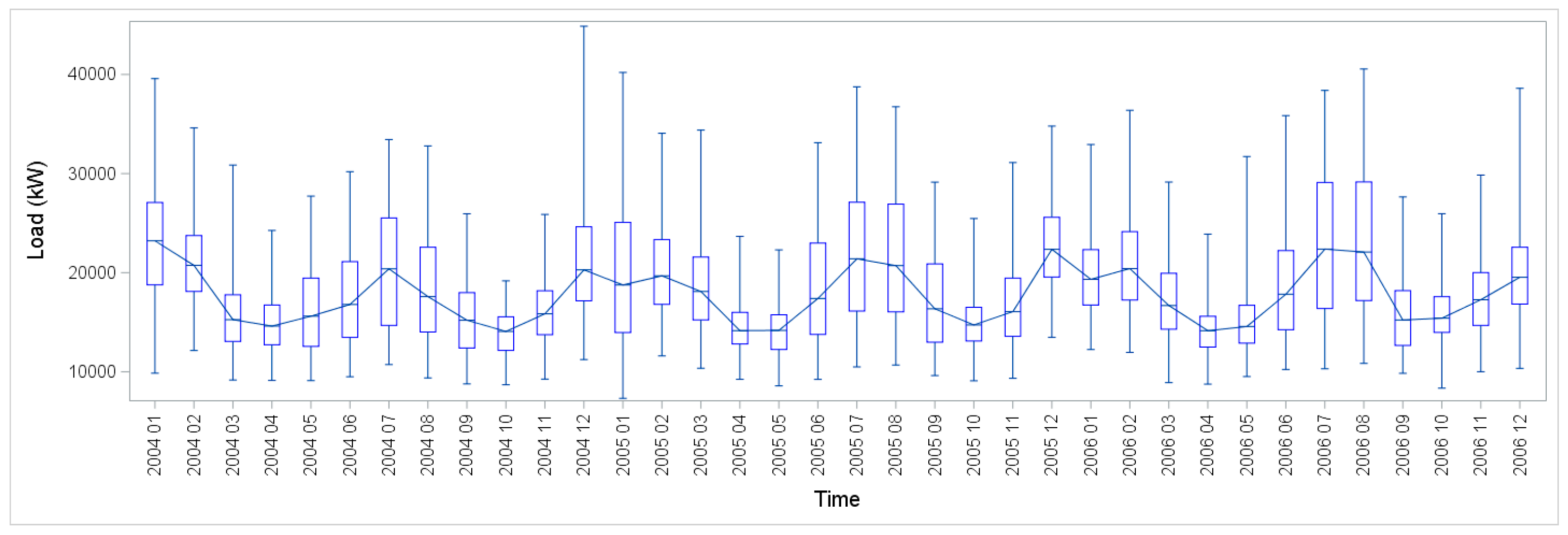
The load data were for the residential and commercial sectors, which typically have a strong correlation with weather variables. Figure 2 shows the scatter plot of temperature vs. load using three years of data (2004 to 2006) from load zone 1 and weather station 6. The graph clearly depicts a strong correlation between the temperature and load. Figure 3 shows the grouped boxplots of load and temperature during the same three years, which illustrate the seasonal patterns of both profiles.

Table 1. Constrained numbered weather stations for each Global Energy Forecasting Competition 2012 (GEFCom2012) load zone.

Zone	Stations
Z1	(6, 10, 2)
Z2	(9, 7, 11, 2, 10, 5)
Z3	(9, 7, 11, 2, 10, 5)
Z4	(7, 2)
Z5	(9, 7, 10)
Z6	(9, 7, 11, 2, 10, 3, 5)
Z7	(9, 7, 11, 2, 10, 5)
Z8	(11, 2, 9, 7)
Z9	(4, 7, 8, 1, 10, 6, 3, 9, 5)
Z10	(1, 3, 5, 4, 7, 6)
Z11	(3, 5, 7, 1)
Z12	(5, 3, 7, 1)
Z13	(2, 11, 6, 10)
Z14	(4, 6, 8, 10, 1)
Z15	(6, 10)
Z16	(7, 3, 9, 10, 5, 6, 1)
Z17	(4, 8, 6, 10, 7, 1)
Z18	(7)
Z19	(10, 6, 7)
Z20	(11, 2, 9, 7, 10, 6)
Z21	(7, 9, 10, 6, 3, 2, 5, 11, 8, 4, 1)

lists the stations selected for each load zone using the weather station selection methodology proposed by [14]. The weather stations are listed from left to right based on the in-sample fit error in ascending order. In this paper, we propose and evaluate alternative methods to combine these selected weather stations for each load zone.

3.2. Results

The heat map in

Table 2. Mean absolute percentage errors (MAPEs) of the load zones under different weather station combination methods.

	Zone	No.	Benchmark	Linear	Exponential	MAPE	G-mean	Twofold	GA	Ensemble
Aggregate	21	11	5.22	5.16	5.28	5.13	5.19	5.22	5.06	5.14
Regular Zones	1	3	7.01	7.17	7.21	7.00	6.99	7.01	7.03	7.04
	2	6	5.62	5.65	5.70	5.62	5.60	5.62	5.59	5.61
	3	6	5.62	5.65	5.70	5.62	5.60	5.62	5.59	5.61
	5	3	9.88	9.56	9.45	9.92	9.85	9.88	10.61	9.84
	6	7	5.55	5.57	5.62	5.56	5.54	5.54	5.54	5.53
	7	6	5.62	5.65	5.70	5.62	5.60	5.62	5.59	5.61
	8	4	7.50	7.41	7.38	7.52	7.48	7.50	7.37	7.43
	10	6	6.70	6.45	6.36	6.72	6.68	6.39	6.46	6.49
	11	4	7.70	7.67	7.69	7.72	7.69	7.70	7.68	7.67
	12	4	6.78	6.62	6.57	6.84	6.76	6.78	6.80	6.69
	13	4	7.39	7.27	7.24	7.40	7.36	7.39	7.51	7.35
	14	5	9.38	9.34	9.27	9.40	9.39	9.38	9.33	9.31
	15	2	7.44	7.42	7.42	7.44	7.44	7.44	7.43	7.43
	16	7	8.12	8.14	8.13	8.14	8.10	8.08	8.15	8.04
	17	6	5.26	5.37	5.52	5.26	5.27	5.26	5.28	5.29
	18	1	6.72	6.72	6.72	6.72	6.72	6.72	6.72	6.72
	19	3	7.90	7.97	7.98	7.90	7.90	7.90	7.92	7.91
	20	6	5.75	5.63	5.61	5.76	5.73	5.72	5.61	5.66
	Average		7.00	6.96	6.96	7.01	6.98	6.97	7.01	6.96
Excluded	4	2	16.08	16.27	16.27	16.08	16.05	16.08	16.12	16.13
Zones	9	9	139.16	139.95	141.73	139.16	139.15	139.17	138.56	139.71

depicts the MAPEs of 21 load zones under all eight different methods including the benchmark from [14] and the seven methods proposed in this paper. A cooler color (green) indicates a lower MAPE value, while a warmer color (red) indicates a higher MAPE value. Following [14] we exclude Zone 4, which experienced a major outage, and Zone 9, which is an industrial customer not responsive to the weather conditions.

The results show a diverse performance of the weather station combination methods in each load zone. Overall, not a single method dominates all zones. At the aggregate level Zone 21, the GA-based combination performed the best, while only one of the seven alternatives, exponential combination underperformed the benchmark. On average for the 18 regular load zones, only two of the seven alternatives, MAPE-based combination and GA-based combination, underperformed the benchmark. These observations suggest that the benchmark, e.g., weighting the selected weather stations equally, has some more accurate alternatives. The ensemble performed the best on average for the 18 regular zones, improving the benchmark by 0.6% on average. The largest improvement was in zone 10, which was a 3% enhancement. Among the five methods that outperformed the benchmark of the regular zones, the ensemble outperformed the other four in the aggregate zone. Between the benchmark and the ensemble on the 18 regular zones plus the aggregate zone, the ensemble won 15 zones, tied 1 zone, and only lost 3 zones. Considering robustness and accuracy together, the ensemble is the best alternative, though it also involves more computational efforts than its counterparts.

4. Conclusions

Weather variables have been used in many load forecasting models. The electric load profiles of residential and commercial customers have shown significant correlation between weather and load. Power companies use weather data as a major source of information to predict future demand. Weather properties such as temperature and relative humidity are provided by the weather stations located in a service zone. Because some service territories are large, some utilities rely on multiple weather stations. Combining multiple weather profiles helps the forecasting model explain more variations of the load spread.

This paper compared several combination methods to address this challenge. Seven different combination methods were compared with the benchmark simple averaging, which was used in [14], through a case study using the data from the load forecasting track of GEFCom2012. The results suggested that several alternatives are more accurate than combining the stations with equal weights. This could be due to many factors such as the distribution of the load data, the geographic distribution of the service territory and the location and number of weather stations. In addition, the ensemble that takes a simple average of different combination methods offers the most robust performance and accurate forecasts.

There are numerous papers that discuss the importance of weather data for load forecasting. This paper is among the first to formally investigate and evaluate different methods for weather station combination. The proposed combination methods are some representative techniques. These techniques could be improved and customized to enhance the load forecasting performance. Future research directions may include other factors such as location information into a combination method to capture the benefits of having multiple weather stations.