Adaptive Comfort Control Implemented Model (ACCIM) for Energy Consumption Predictions in Dwellings under Current and Future Climate Conditions: A Case Study Located in Spain

Abstract

Currently, the knowledge of energy consumption in buildings of new and existing dwellings is essential to control and propose energy conservation measures. Most of the predictions of energy consumption in buildings are based on fixed values related to the internal thermal ambient and pre-established operation hypotheses, which do not reflect the dynamic use of buildings and users’ requirements. Spain is a clear example of such a situation. This study suggests the use of an adaptive thermal comfort model as a predictive method of energy consumption in the internal thermal ambient, as well as several operation hypotheses, and both conditions are combined in a simulation model: the Adaptive Comfort Control Implemented Model (ACCIM). The behavior of ACCIM is studied in a representative case of the residential building stock, which is located in three climate zones with different characteristics (warm, cold, and mild climates). The analyses were conducted both in current and future scenarios with the aim of knowing the advantages and limitations in each climate zone. The results show that the average consumption of the current, 2050, and 2080 scenarios decreased between 23% and 46% in warm climates, between 19% and 25% in mild climates, and between 10% and 29% in cold climates by using such a predictive method. It is also shown that this method is more resilient to climate change than the current standard. This research can be a starting point to understand users’ climate adaptation to predict energy consumption.

1. Introduction

Concerns on the environmental degradation of the planet are increasing because it implies global warming and the extinction of animals [1], thus leading to the proposal of guidelines and standards to regulate resource depletion and the emission of pollutant gases to the atmosphere. Regarding the building sector, the European Union set the need for reducing such gases by 90% by 2050 [2]. This need for reducing the emissions of pollutant gases is due to the significant impact of the building sector on the environment. In this sense, buildings are responsible for between 30% and 40% of the total energy consumption in the planet [3,4], and 40% of the emission of pollutant gases to the atmosphere [5,6]. Such percentages are mainly because of their deficient energy performance [7,8,9,10], although other aspects, such as users’ behavior [11], are influential factors as well.

In countries of southern Europe, most of the existing building stock was built in periods before the implementation of the first normatives for energy efficiency of buildings [12,13,14]. Regarding the deficient energy performance, the effect of climate change should also be considered [15,16]. Such an effect can imply the increase of CO₂ emissions by 12% and the cooling energy consumption by 120% due to the use of heating, ventilation, and air-conditioning (HVAC) systems [17,18], since the main problem of the energy analysis of buildings is the use of historical climate data without considering the increase of external temperatures in the following years [19]. There are studies analyzing the influence of climate change on the energy demand of buildings. Pérez-Andreu et al. [15] analyzed various energy conservation measures of the façade of a building located in the Mediterranean region. The results showed how the cooling demand and the risk of overheating increased in future scenarios. The increase of cooling demand was obtained in studies conducted in different regions: (i) Karimpour et al. [20] analyzed the effect of climate change in a case study located in Adelaide (Australia). The results demonstrated that the effect of climate change increased the need of establishing measures to reduce the cooling demand; (ii) Kalvelage et al. [21] analyzed several kinds of buildings (e.g., hospitals, hotels, and supermarkets) located in the cities of Atlanta, Los Angeles, Baltimore, Seattle, and Phoenix. The results reflected a decrease in heating demand and an increase in cooling demand; (iii) Rubio-Bellido et al. [22] studied the influence of climate change in office buildings located in nine climate zones of Chile. In the buildings analyzed, heating demand decreased between 0.54 and 2.62 kWh/year, whereas cooling demand increased between 0.53 and 4.47 kWh/year.

The building sector should, therefore, adapt to this new situation [23] by establishing efficient strategies in order to reduce cooling energy demand and, in turn, its environmental impact. In this way, the setpoint temperatures assigned to HVAC systems directly influence the energy consumption of buildings [24] because they determine the working periods and range of the active systems. The configuration of acceptable setpoint temperatures would reduce the environmental impact of buildings, thus guaranteeing appropriate thermal comfort conditions without the need of realizing a high economic investment [25]. Numerous authors analyzed the influence of setpoint temperatures on the energy performance of buildings in different climate zones: (i) Hoyt et al. [26] used setpoint temperatures of 27.87 °C and 18.3 °C for upper and lower limits of the HVAC system of an office building located in the cities of Baltimore, Chicago, Duluth, Fresno, Miami, Phoenix, and San Francisco. The use of such setpoint temperatures allowed a saving between 32% and 73% to be achieved in the energy consumption; (ii) Wan et al. [27] analyzed the use of optimal setpoint temperatures to reduce the energy consumption in office buildings of Hong Kong. The results showed that the cooling setpoint temperatures greater than 25.5 °C obtained significant savings in the cooling demand, both in current and future scenarios; (iii) Parry et al. [28] studied how an increase between 2 °C and 4 °C in the cooling setpoint temperature in an office building in Zurich would result in a three-fold decrease in the annual energy consumption; (iv) Spyropoulos and Balaras [29] analyzed the reliability of saving the energy consumption in bank branch offices by modifying the setpoint temperatures. A temperature of 20 °C for the lower limit and 26 °C for the upper limit allowed a reduction of 45% in the total energy consumption to be achieved.

However, in the research studies mentioned above, those setpoint temperatures of comfort models based on the predicted mean vote (PMV) index were always configured such that temperatures were fixed and did not depend on the external temperature. Unlike such models, adaptive comfort models consider that occupants can take actions to adapt themselves to the thermal ambient, as well as establish comfort limits depending on the external temperature, thereby varying periodically. These adaptive setpoint temperatures could be established using external probes or weather stations [30]. Many studies on this field were conducted, covering topics ranging from the development of comfort models [31] to the evaluation of comfort conditions of the main standards in those future scenarios influenced by climate change [32].

Unlike the variation of fixed setpoint temperatures, there are no many studies on the variation of adaptive setpoint temperatures: (i) Van der Linden et al. [33] used the lower limit of a comfort model established in the ISSO74 standard [34] for the Netherlands. The results obtained a reduction of 74% in energy consumption [35]; (ii) in Spain, setpoint temperatures based on the simplified method of the ASHRAE 55-2013 standard [36] were applied, that is, using setpoint temperatures monthly varying according to the external average temperature. The results estimated a decrease of 20% and 80% in heating and cooling, respectively [37]; (iii) in other studies, neutral temperatures of a comfort model for mixed-model buildings, which was developed for the climate of Seville [38], were used as setpoint temperatures to compare later the energy consumptions from the use of adaptive and conventional setpoint temperatures (i.e., used before the study). The results showed energy savings of 11.4% in heating and 27.5% in cooling. The average heating and cooling adaptive setpoint temperatures were 21.5 °C and 24 °C, whereas the conventional temperatures were 22.3 °C and 23.5 °C, respectively [39]; (iv) unlike this study where neutral temperatures were used as setpoint temperatures, the energy consumption in mixed-model buildings were quantified in another study by using the adaptive comfort limits from the EN15251 standard [40] as setpoint temperatures in the current scenario and under the influence of climate change [41]. The results showed a decrease of the energy consumption between 59.5% and 36.7% by comparing the use of conventional setpoints (23 °C in heating and 25 °C in cooling) with the use of adaptive setpoints, respectively, between the current and 2080 scenarios.

In Spain, the comfort model currently set by the Spanish Building Technical Code (CTE: its acronym in Spanish) [42] for residential buildings establishes both very restrictive setpoint temperatures and standardized usage schedules of HVAC systems without considering the various climate zones. Furthermore, such q way of operation causes high energy consumption mainly due to the main and setback setpoint temperatures of 20 °C and 17 °C in heating, and 25 °C and 27 °C in cooling. On the other hand, the CTE uses the same comfort model with the same setpoints and usage schedules for all climate zones of the country.

Human adaptation depends on social, physiological and psychological behavior, and this has an important effect on the achievement of thermal comfort and, therefore, energy consumption. In fact, in Seville, there are some people who cannot open the windows to ventilate at night for security reasons. The differences between simulated and actual human behavior are the cause of the main discrepancies between simulated and actual energy consumption [43]. Currently, CTE’s comfort model is based on the PMV index; therefore, it does not consider the human adaptation to the changing thermal environment. Also, equipment usage schedules from CTE might not be similar to the actual average schedules; thus, there could be some uncertainty in simulated energy consumption results if compared with actual energy consumptions.

To maintain high thermal comfort levels and reduce the energy consumption, this research suggests the use of a comfort model which considers setpoint temperatures based on the adaptive comfort model from the EN15251 standard within its application range, and setpoint temperatures based on different static comfort models when the adaptive comfort model is outside such a range. Hence, several operation hypotheses of heating and cooling setpoints are evaluated and compared to the current predictive standards. Models are used in three climate zones which represent current and future (2050 and 2080) climate scenarios. This case study is a residential building representative of the building stock in Spain and is related to the main problems of energy poverty in the country [44].

2. Methodology

The methodology is based on the six stages shown in the following sections (Figure 1): (i) data collection; (ii) development of the comfort models; (iii) analysis of the climate zones; (iv) definition of the case study; (v) simulations performed in current and future scenarios; and (vi) results.

2.1. Data Collection

To study the potential of the adaptive comfort model, it is required to establish the setpoint temperatures which fix the limits of the internal temperatures from which air-conditioning systems in the dwelling start to work.

The setpoint temperatures in the static model are set according to the CTE [42]. However, the procedure to obtain the adaptive setpoint temperatures is more complex. The adaptive setpoint temperatures correspond with the adaptive comfort limits from the EN15251 standard [40], which in turn depend on the running mean outdoor temperature. The running mean outdoor temperature is calculated by using Equation (1).

$${\mathsf{\theta }}_{rm}=\left({\mathsf{\theta }}_{ed-1}+0.8\ast {\mathsf{\theta }}_{ed-2}+0.6\ast {\mathsf{\theta }}_{ed-3}+0.5\ast {\mathsf{\theta }}_{ed-4}+0.4\ast {\mathsf{\theta }}_{ed-5}+0.3\ast {\mathsf{\theta }}_{ed-6}+0.2\ast {\mathsf{\theta }}_{ed-7}\right)/3.8,$$

(1)

where Ɵ_Ed−1 is the daily average external air temperature of the previous day, Ɵ_Ed−2 is the daily average external air temperature of two days before, and so on.

The EN15251 standard establishes different categories (

Table 1. Expectation categories addressed in EN15251.

Category	Detail
I	High level of expectation, recommended for spaces occupied by weak and sensitive people with special requirements, such as handicapped, sick, elderly, and very young children.
II	Normal level of expectation; it should be used for new and renovated buildings.
III	Acceptable and moderate level of expectation; it can be used in existing buildings.
IV	Values outside of the criteria of the preceding categories. This category should only be accepted during a limited part of a year.

) in which the level of expectation of the thermal ambient of the occupant is determined. Moreover, the extent of the comfort range depends on such categories. In this case study, as it is an existing building, category III is the appropriate category. For such a category, the adaptive comfort limits are calculated by Equations (2) and (3).

$${\mathsf{\theta }}_{i max}=0.33\times {\mathsf{\theta }}_{rm}+18.8+4,$$

(2)

$${\mathsf{\theta }}_{i min}=0.33\times {\mathsf{\theta }}_{rm}+18.8-4,$$

(3)

where ${\mathsf{\theta }}_{i max}$ is the temperature of the upper limit, ${\mathsf{\theta }}_{i min}$ is the temperature of the lower limit, ${\mathsf{\theta }}_i$ is the internal operative temperature, and ${\mathsf{\theta }}_{rm}$ is the average external working temperature.

This comfort model can be used if some limitations are fulfilled. Regarding the temperature, the average external working temperature should be between 10 °C and 30 °C for the upper comfort limit, and between 15 °C and 30 °C for the lower limit. It should be considered that the graphic is based on a database limited for average external working temperatures higher than 25 °C. Moreover, the upper comfort limit can be extended to around 3.5 °C by increasing the air speed to 1.5 m/s. On the other hand, regarding the occupant, the metabolic activity should be between 1.0 and 1.3 met, and the level of clo between 0.5 and 1. Such a comfort model considers the opportunities of the occupant’s adaptation to the thermal ambient. Therefore, it can be applied to buildings where the opening and closing of windows is possible, as well as where occupants can adapt their clothing to their needs.

2.2. Models

Four different comfort models were suggested for this study: (a) a static model based on the setpoints of the CTE, and (b) three adaptive models: OUT-CTE, OUT-SEN15251, and OUT-AEN15251. In the adaptive models, adaptive heating setpoint temperatures (AHST) and adaptive cooling setpoint temperatures (ACST) are used, which correspond with the comfort limits for Category III in the EN15251 standard when the comfort model is applied. Currently, the use of the static model based on the setpoints of the CTE generates high energy consumptions due to the use of very restrictive setpoint temperatures. Thus, the use of the adaptive models OUT-CTE, OUT-SEN15251, and OUT-AEN15251 could reduce the energy consumption and maintain high comfort levels. When the adaptive thermal comfort model cannot be applied, the following configurations are used: (i) for OUT-CTE, the setpoint temperatures of the CTE are used; (ii) for OUT-SEN15251, the static setpoint temperatures of the EN15251 standard are used (they are included in Table A.3 of the EN15251 standard (i.e., when the running mean outdoor temperature is lower than 10 °C, heating and cooling setpoints are 18 °C and 25 °C, respectively, and when the running mean outdoor temperature is higher than 30 °C, setpoints are 22 °C and 27 °C, respectively); and (iii) for OUT-AEN15251, maximum and minimum comfort limits of the EN15251 standard are used as static setpoint temperatures in its adaptive model, extending horizontally the maximum and minimum comfort limits (i.e., the internal operative temperatures which correspond to average external working temperatures of 30 °C for the upper limit, and 15 °C for the lower limit).

Table 2. Setpoint temperatures used in each model.

Model	Standard	Limit	Range	Setpoint Temperature (°C)
				January–May			June–September			October–December
				24–7	8–15	16–23	24–7	8–15	16–23	24–7	8–15	16–23
Static model	CTE	Upper limit	all	-	-	-	27	-	25	-	-	-
		Lower limit	all	17	20	20	-	-	-	17	20	20
Adaptive model OUT-CTE	EN15251Cat. III CTE	Upper limit (ACST)	${\mathsf{\theta }}_{rm}$ < 10 °C	-	-	-	27	-	25	-	-	-
			10 °C ≤ ${\mathsf{\theta }}_{rm}$ < 30 °C	-	-	-	(1)	-	(1)	-	-	-
			${\mathsf{\theta }}_{rm}$ > 30 °C	-	-	-	27	-	25	-	-	-
		Lower limit (AHST)	${\mathsf{\theta }}_{rm}$ < 15 °C	17	20	20	-	-	-	17	20	20
			15 °C ≤ ${\mathsf{\theta }}_{rm}$ ≤ 30 °C	(2)			-	-	-	(2)
			${\mathsf{\theta }}_{rm}$ > 30 °C	17	20	20	-	-	-	17	20	20
Adaptive model OUT-SEN15251	EN15251 Cat. III	Upper limit (ACST)	${\mathsf{\theta }}_{rm}$ < 10 °C	-	-	-	25	-	25	-	-	-
			10 °C ≤ ${\mathsf{\theta }}_{rm}$ < 30 °C	-	-	-	(1)	-	(1)	-	-	-
			${\mathsf{\theta }}_{rm}$ > 30 °C	-	-	-	27	-	27	-	-	-
		Lower limit (AHST)	${\mathsf{\theta }}_{rm}$ < 15 °C	18			-	-	-	18
			15 °C ≤ ${\mathsf{\theta }}_{rm}$ ≤ 30 °C	(2)			-	-	-	(2)
			${\mathsf{\theta }}_{rm}$ > 30 °C	22			-	-	-	22
Adaptive model OUT-AEN15251	EN15251 Cat. III	Upper limit (ACST)	${\mathsf{\theta }}_{rm}$ < 10 °C	-	-	-	26.10	-	26.10	-	-	-
			10 °C ≤ ${\mathsf{\theta }}_{rm}$ < 30 °C	-	-	-	(1)	-	(1)	-	-	-
			${\mathsf{\theta }}_{rm}$ > 30 °C	-	-	-	32.70	-	32.70	-	-	-
		Lower limit (AHST)	${\mathsf{\theta }}_{rm}$ < 15 °C	19.75			-	-	-	19.75
			15 °C ≤ ${\mathsf{\theta }}_{rm}$ ≤ 30 °C	(2)			-	-	-	(2)
			${\mathsf{\theta }}_{rm}$ > 30 °C	24.70			-	-	-	24.70

Notes: ACST: adaptive cooling setpoint temperature; AHST: adaptive heating setpoint temperature; CTE: Spanish Building Technical Code. (1) $0.33\times {\mathsf{\theta }}_{rm}+18.8+4$; (2) $0.33\times {\mathsf{\theta }}_{rm}+18.8-4$.

and Figure 2 show such setpoint temperatures. In addition, the values of the setpoint temperatures vary in schedule ranges (12:00–7:00 a.m., 8:00 a.m.–3:00 p.m., and 4:00–11:00 p.m.) in the CTE static model. To make representative comparisons, such values also varied in the OUT-CTE model. Also, it is advisable to consider that the working schedule of the air-conditioning equipment set in the CTE was used to establish a coherent comparison between the static model set in the CTE and the adaptive models proposed. In this way, the cooling mode works from June to September, between 4:00 p.m. and 7:00 a.m., whereas the heating mode works from January to May and from October to December throughout the day.

The EN15251 adaptive model establishes that the thermal comfort can be achieved by using ventilation and by the occupant’s adaptation actions if the running mean outdoor temperature fulfils the conditions of applicability, as well as other conditions related to the HVAC systems and the levels of both clo and met. If the thermal comfort is not achieved, it would be necessary to activate the HVAC systems and use setpoint temperatures from the static model of the EN15251 standard. Therefore, when the running mean outdoor temperature is higher than 30 °C, the upper and lower limits vary from 32.70 °C to 27 °C, and from 24.70 °C to 22 °C, respectively. Also, when the running mean outdoor temperature is lower than 10 °C, the upper and lower limits vary from 26.10 °C to 25 °C, and from 19.70 °C to 18 °C, respectively. For this reason, various static models are used when the conditions of applicability of the adaptive model are not fulfilled.

2.3. Analysis of Climate Zones

In this paper, the three most representatives climate zones of the Spanish territory set in the CTE DB HE (which is the Spanish Building Technical Code document in relation to energy savings) reference climates were considered [45]: (i) the B4 climate zone, which belongs to class Csa according to Köppen–Geiger’s classification [46] (Mediterranean climate, with mild winters and dry and very hot summers), in which the city of Seville is located; (ii) the D3 climate zone, which belongs to class BSh (cold semi-arid climate, with moderated cold winters and hot summers), in which the city of Madrid is located; and (iii) the E1 climate zone, which belongs to class Csb (continental Mediterranean climate, with mild summers and cold winters), in which the city of Ávila is located. Such climates were selected with the aim of obtaining results which were extrapolated to other countries with the same climate zones.

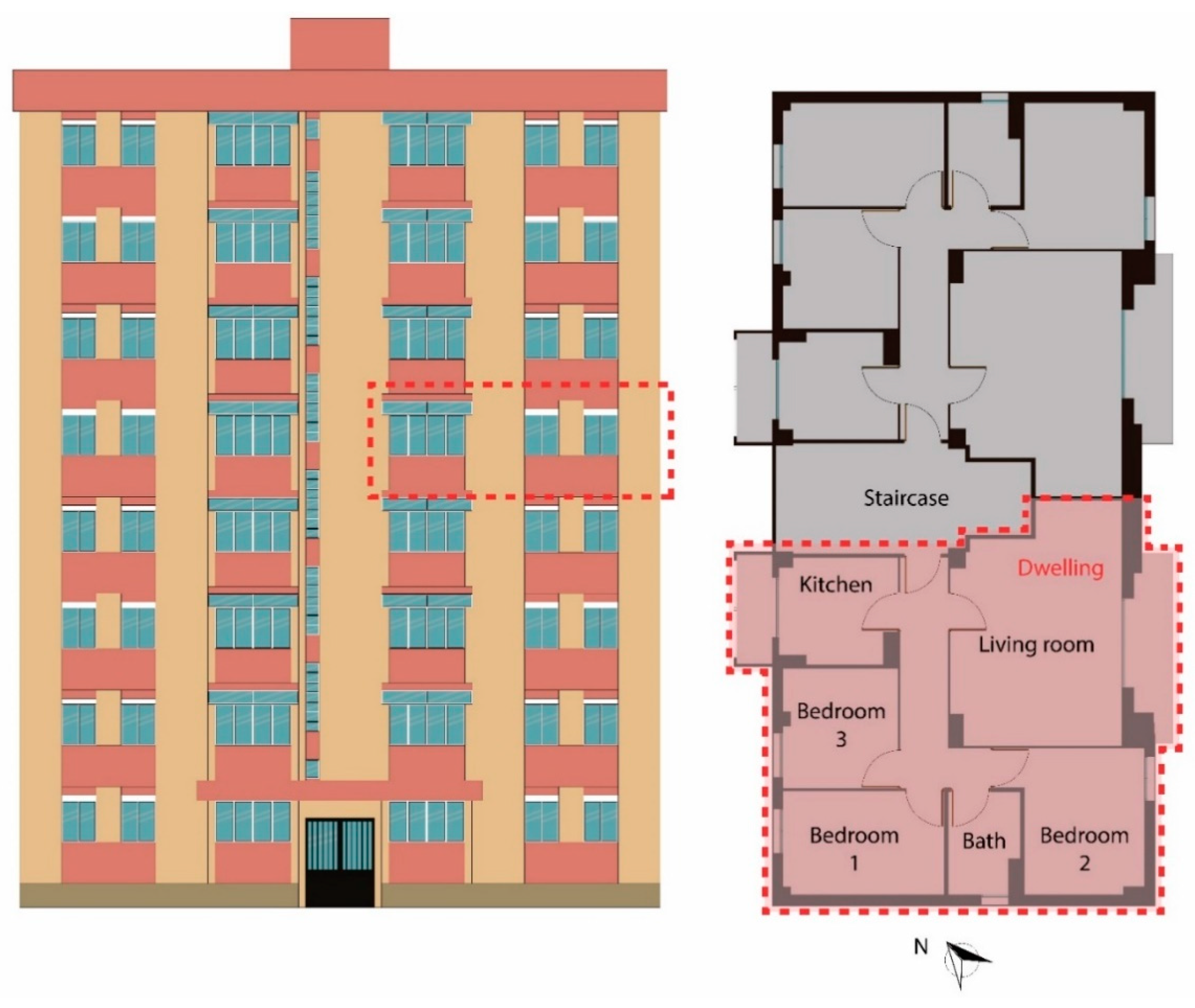
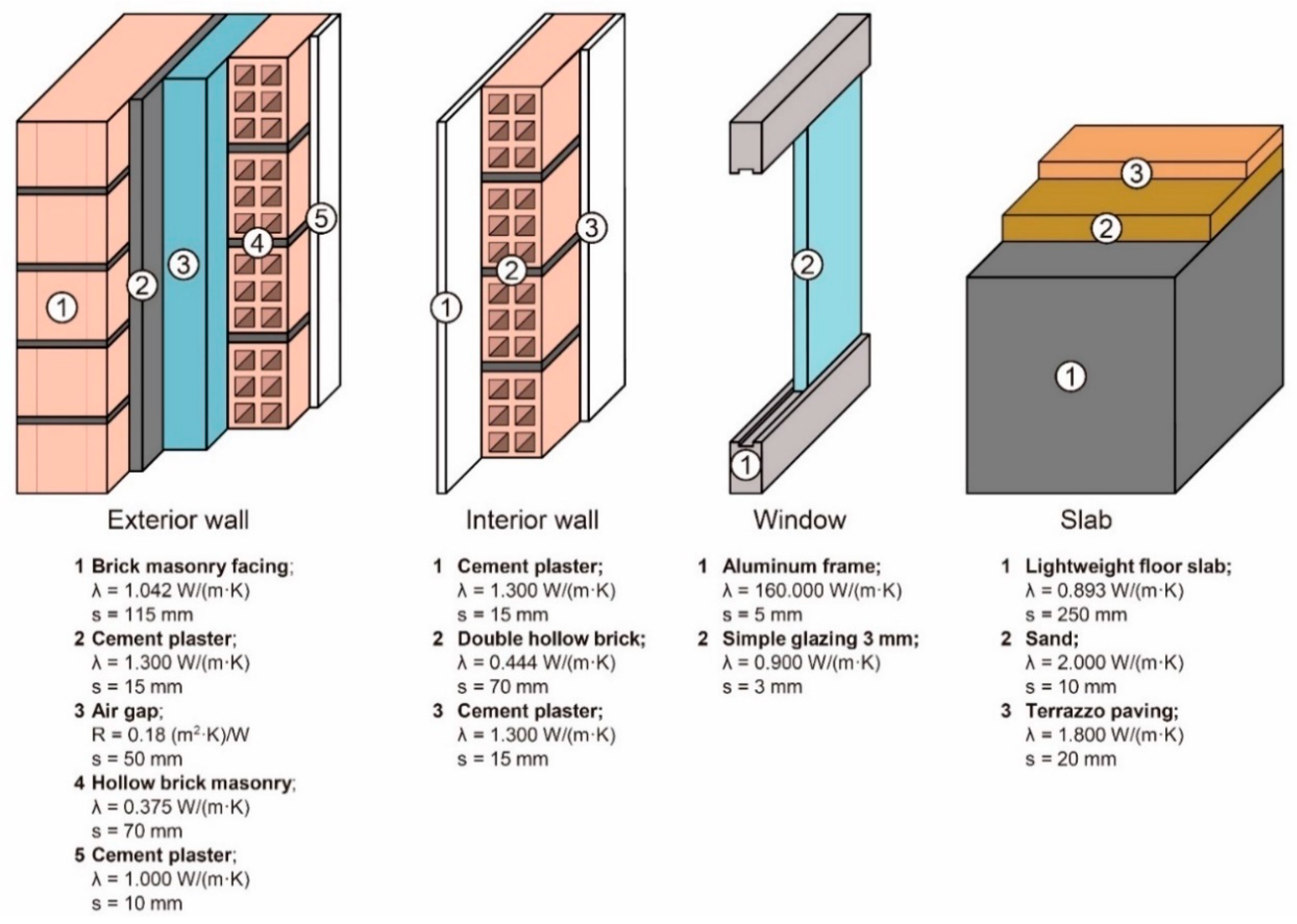
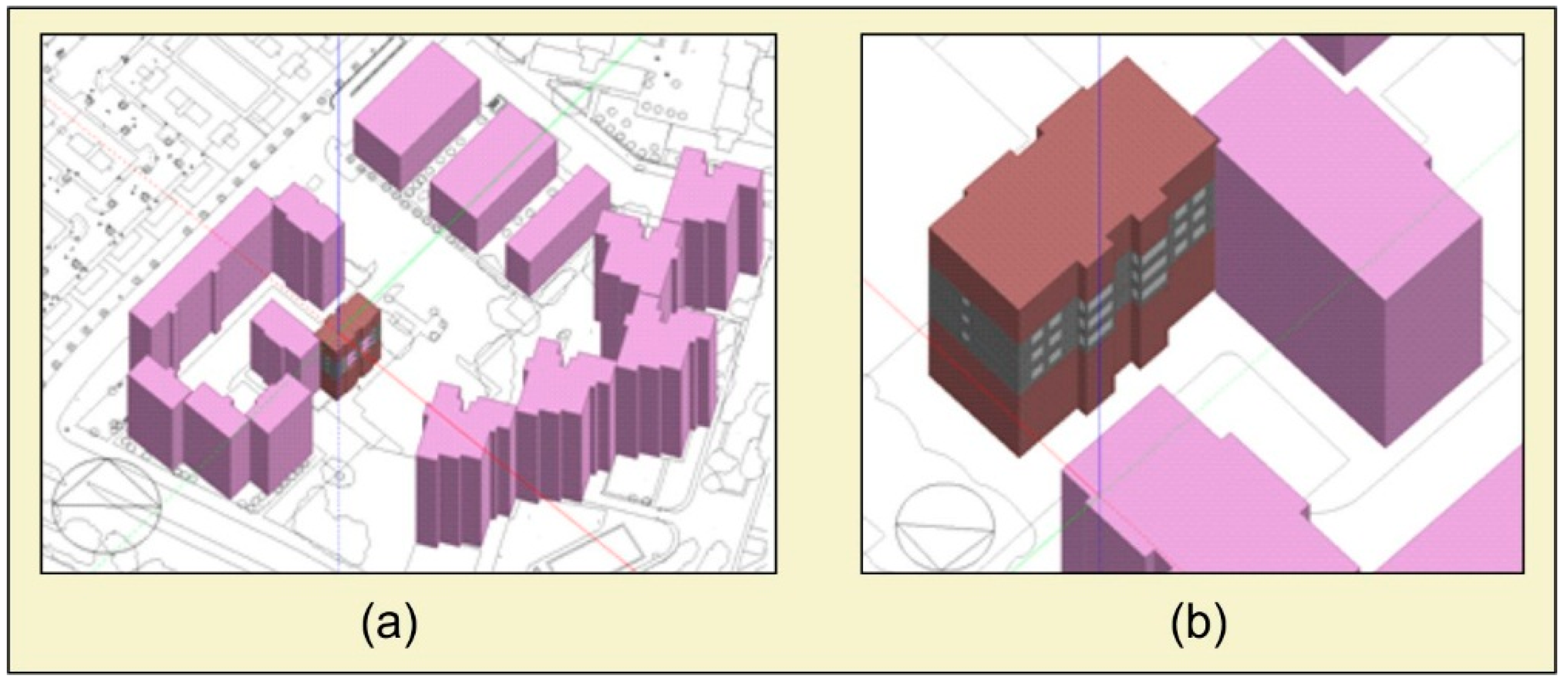
2.4. Definition of the Case Study

The case study was an apartment located on the fourth floor of a residential building of eight floors, which was built in 1973 with a surface area of 77 m². The apartment has a living room, a kitchen, a bathroom, and three bedrooms. Figure 3 shows the building and the dwelling studied in red.

According to data from the National Institute of Statistics (INE: its acronym in Spanish) [12], 5.121 million dwellings (i.e., 27.7% of the total) in Spain have a surface area of 76–90 m², and most dwellings (1.047 million) were built between 1971 and 1980. The typology of the case study is, therefore, statistically representative.

This dwelling was studied in a previous research paper [32]. In this study, the simulation model met the limits of 10% and 30% on Mean Bias Error (MBE) and Coefficient of Variation of the Root Square Mean Error (CV (RSME)) as per ASHRAE Guideline 14 [47] and, thus, the simulation model was validated. The dwelling has a heat pump with an energy efficiency ratio (EER) of 2.00, and with a coefficient of performance (CoP) of 2.10.

Figure 4 shows the constructive characteristics of the building selected. The envelope was used in many buildings between 1960 and 1980, a period when many residential buildings were built. Also, considering that the incorporation of thermal insulation was not mandatory until 1979 [48], the building selected (which was built in 1973) does not have thermal insulation in the envelope.

The operation schedules used are defined as per CTE for residential use (Figure 5). The occupation on working days varies throughout the day, reaching 100% from 12:00 to 7:00 a.m. On the weekend, a total and constant occupation is shown. The use of equipment and lighting reaches 100% between 8:00 p.m. and 11:00 p.m.

Table 3. Internal loads.

Internal Loads	W/m2 at 100%
Sensible occupancy	2.15
Latent occupancy	1.36
Lighting	4.40
Equipment	4.40

indicates the maximum values for the internal loads, which were obtained from the CTE’s reference values to be used in building energy performance simulations.

During the summer, it is estimated that the inhabitable spaces present a ventilation of four renovations per hour between 1:00 a.m. and 8:00 a.m. by opening the windows. During the remaining periods, the minimum volume of external ventilation air for residential use should be applied according to the CTE. Our case study is a dwelling of three bedrooms, with a minimum volume in dry rooms of 8 L/s in the main bedroom, 4 L/s in the remaining bedrooms, and 10 L/s in the living room. In wet rooms, the minimum volume per room should be 8 L/s.

2.5. Simulation in Current and Future Scenarios

Simulations were performed using DesignBuilder software because it includes EnergyPlus (a calculation engine), which develops advanced dynamic simulations by using schedule weather data files of each climate zone under study. Figure 6 shows the model developed in DesignBuilder, in which the environment of the building (a) and upper and lower floors of the dwelling under study (b) were modeled to obtain accurate results. The dwelling was modeled by in situ measurements, developing a very real envelope of façades and gaps (according to the constructive characteristics in Figure 4) and considering the operation hypothesis and the internal loads set in the CTE (according to Figure 5 and Table 3). Moreover, the adaptive setpoint temperatures included in Table 2 were applied by using Compact Schedules.

In this study, the application of adaptive setpoints in future climate scenarios was also evaluated. For this purpose, the CCWorldWeatherGen tool of the United Kingdom (UK) Met Office Hadley Centre Coupled Model 3 (HadCM3) was used because it generates weather files which are adapted to the climate change of any place in the world, as well as files compatible with most building performance simulation programs [49]. The morphing of the three current climate files (B4, D3 E1) was carried out for the A2 scenario of greenhouse gas emissions, which is considered medium–high by the Intergovernmental Panel on Climate Change (IPCC), resulting in climate scenarios files for 2050 and 2080. By using this method, files of the Energy Plus Weather (EPW) climate of the place in question were obtained, and then the morphing process was carried out with projections of the GMC (general circulation model). In such a morphing process, the A2a, A2b, and A2c guidelines of the HadCM3 model were combined.

One of the advantages of the morphing process is the change of monthly mean climate values to show future variations, while maintaining the underlying characteristics of the current climate. In this way, the coherence with historic data is maintained, and buildings in current and future climates can be directly compared. Regarding the disadvantages, some variables are produced independently; hence, the relationship between them and the new climate files could not be the same, as in the historic files [18]. In addition, this method has the following limitations: (i) it should be considered that the resolution of HadCM3 is mainly used on a global scale; (ii) the HadCM3 model covers a finite grid point model covering an area of 2.5° latitude by 3.75° longitude, with a resolution of around 300 × 300 km² in the whole world; (iii) this method does not consider the microclimate effects typical of the cities (e.g., urban heating island) because the weather stations, which record data to be used for generating climate files, are generally located in the outskirts of the cities; and (iv) this method does not consider extraordinary natural phenomena because it only estimates future tendencies from average values.

Figure 7 shows the increase in the average temperature of daily minimum and maximum temperatures, and the variation of the relative humidity due to climate change. The annual average temperature increases in B4, D3, and E1 scenarios from 18.7 °C to 22.5 °C, from 14.7 °C to 18.5 °C, and from 11.6 °C to 15.4 °C, respectively. However, as can be seen in such three climate zones, the effects of global warming do not equally influence throughout the year, as the increase in temperature and the respective decrease in humidity are less in cold months than in warm months. January shows an increase in the average minimum and maximum temperatures of 2.3 °C and 2.5 °C, respectively, whereas in July there are increases of 5.2 °C and 7.4 °C, respectively. Regarding the variation of the relative humidity, the variation in the average maximum and minimum temperatures is the same throughout the year, except in July. While in January, both minimum and maximum averages are decreased by 2%, the average of the minimum temperatures is reduced by 13.8% and the average of the maximum temperatures is reduced by 15.9% in July.

The comfort model set in the EN15251 standard allows the comfort levels to be evaluated only in the current scenario. In this way, as there are no comfort models available for future scenarios, the comfort model of the EN15251 standard was used for the climate scenarios of 2050 and 2080. This could imply a limitation because the acceptability and comfort ranges could change as the human beings adapt to the increase in temperature. Thus, the calculation of the comfort levels and the adaptive energy consumption is limited because the adaptation of the temperature increase was not considered. However, it is possible that the potential of energy saving grows. This is due to the fact that, if the adaptation to future scenarios is considered, human beings might consider higher temperatures acceptable; thus, the adaptive setpoint temperatures could be higher than those of the current scenario [41].

3. Results and Discussion

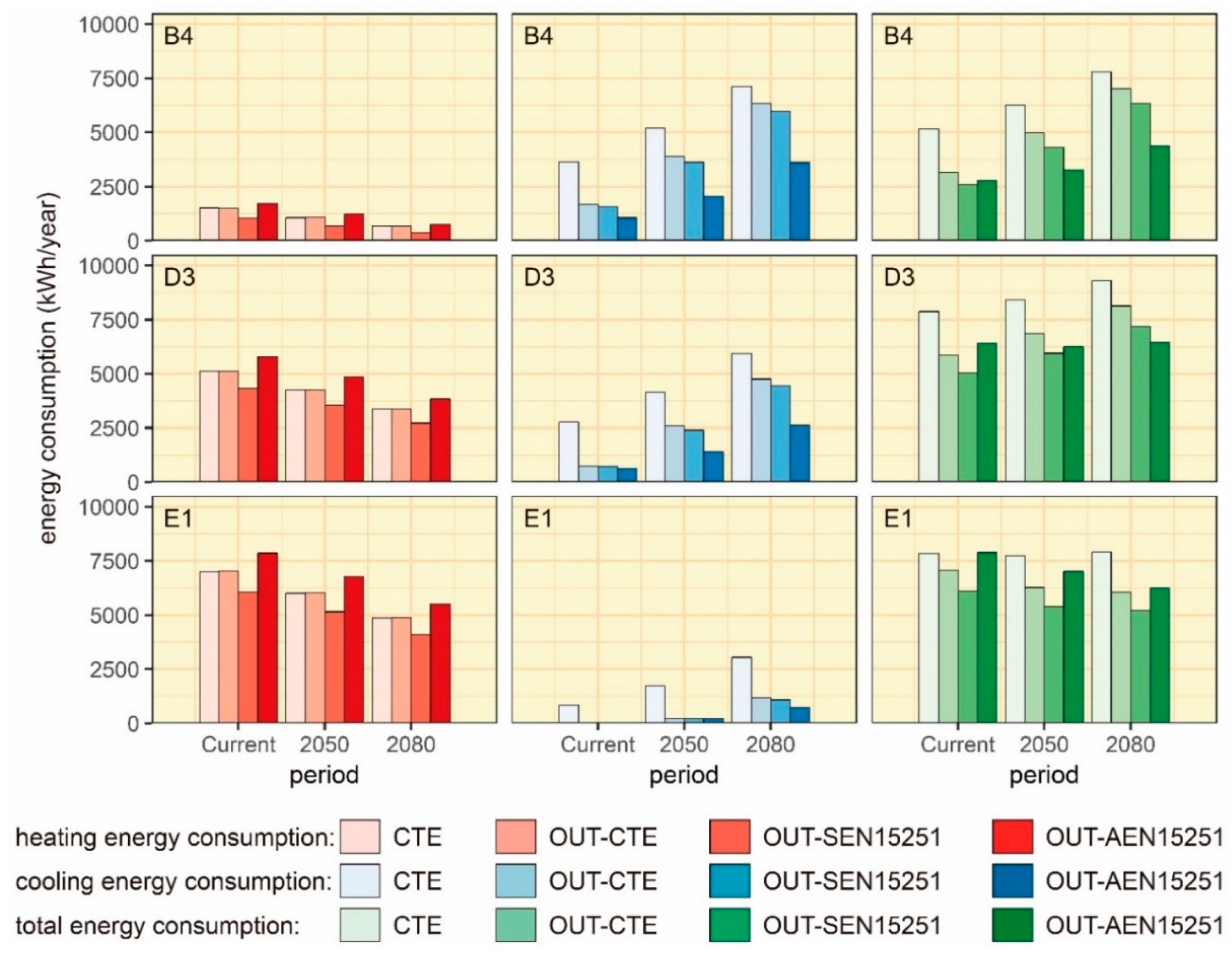
3.1. Influence of Adaptive Comfort Control Implemented Model (ACCIM) on the Annual Energy Consumption

The energy consumption was analyzed by using different adaptive comfort models in various climate zones and scenarios. To evaluate the adaptive comfort models proposed globally, the averages of the reduction of the total energy consumption (heating and cooling) were determined with respect to the static model set in the CTE in the climate scenarios.

Table 4. Reduction of the total energy consumption with respect to the CTE.

Zone	Models
	OUT-CTE	OUT-SEN15251	OUT-AEN15251
B4	23%	33%	46%
D3	19%	29%	25%
E1	17%	29%	10%

shows such averages according to each climate zone. In this way, the OUT-AEN15251 model globally provided the greatest consumption reductions in B4 (46%), whereas the OUT-SEN15251 model gave the greatest reductions in D3 (29%) and E1 (29%). This was mainly due to the fact that the setpoint temperatures were greater in the OUT-AEN15251 model; thus, they adapted better to the warm climate of B4, whereas the OUT-SEN15251 model adapted better to D3 and E1, which were the least warm climates. On the other hand, the OUT-CTE model provided the most unfavorable results in B4 and D3 because of the restrictive cooling setpoint temperature of 25 °C applied during the hottest hours of the day.

Nevertheless, such results were analyzed in detail (Figure 8 and

Table 5. Reduction of the consumption of the adaptive models.

Climatic Zone Scenario			CTE	OUT-CTE		OUT-SEN15251		OUT-AEN15251
			kWh/m²·Year	kWh/m²·Year	Reduction (%)	kWh/m²·Year	Reduction (%)	kWh/m²·Year	Reduction (%)
B4	Current	Cooling	3652.45	1682.26	54%	1561.01	57%	1065.81	71%
		Heating	1504.85	1484.04	1%	1040.56	31%	1727.15	−15%
		Total	5157.30	3166.30	39%	2601.57	50%	2792.96	46%
	2050	Cooling	5196.55	3904.71	25%	3626.22	30%	2052.95	60%
		Heating	1060.49	1078.04	−2%	695.50	34%	1220.57	−15%
		Total	6257.04	4982.75	20%	4321.72	31%	3273.52	48%
	2080	Cooling	7116.07	6351.04	11%	5962.58	16%	3616.59	49%
		Heating	687.07	673.17	2%	385.79	44%	759.12	−10%
		Total	7803.14	7024.22	10%	6348.36	19%	4375.71	44%
D3	Current	Cooling	2773.06	745.89	73%	722.83	74%	640.52	77%
		Heating	5105.23	5113.53	0%	4323.58	15%	5778.52	−13%
		Total	7878.28	5859.42	26%	5046.41	36%	6419.04	19%
	2050	Cooling	4150.70	2595.82	37%	2395.47	42%	1399.97	66%
		Heating	4273.92	4260.92	0%	3556.26	17%	4851.81	−14%
		Total	8424.62	6856.73	19%	5951.73	29%	6251.78	26%
	2080	Cooling	5931.86	4762.16	20%	4448.74	25%	2624.20	56%
		Heating	3368.92	3371.96	0%	2729.79	19%	3835.79	−14%
		Total	9300.78	8134.12	13%	7178.54	23%	6459.99	31%
E1	Current	Cooling	844.63	37.54	96%	37.72	96%	37.72	96%
		Heating	7005.40	7037.78	0%	6079.29	13%	7864.73	−12%
		Total	7850.02	7075.32	10%	6117.01	22%	7902.45	−1%
	2050	Cooling	1738.24	229.21	87%	228.41	87%	228.41	87%
		Heating	6010.11	6038.63	0%	5159.90	14%	6785.03	−13%
		Total	7748.36	6267.84	19%	5388.31	30%	7013.44	9%
	2080	Cooling	3046.99	1174.32	61%	1090.36	64%	742.19	76%
		Heating	4863.72	4876.70	0%	4117.06	15%	5510.47	−13%
		Total	7910.71	6051.02	24%	5207.42	34%	6252.65	21%

), including those of the static model according to the CTE. The results obtained from the heating, cooling, and total consumption were analyzed, as well as the results according to the climate zone. Moreover, the percentages of reduction in energy consumption with respect to the static model of the CTE are shown.

Regarding the heating consumption, the greatest total energy consumption was in the CTE-AEN15251 model in the three climate zones, both in current and future scenarios, mainly due to the fact that, outside the applicability limits, the lower limit of temperature was 19.75 °C and that such a model continuously had the highest heating setpoint temperature. B4 presented the lowest heating consumption because the temperatures in this zone were closer to such a limit.

As for cooling, the greatest energy consumption was obtained by using static setpoints (CTE model) and the lowest energy consumption was obtained with the OUT-AEN15251 model because of the setpoint temperatures used: the static model of the CTE establishes the setpoint temperature of 25 °C in daytime hours, whereas the OUT-AEN15251 model establishes 32.70 °C as the highest. In this case, B4 presented the greatest cooling consumption because it had the highest temperatures.

With respect to the total consumption for the current scenario, the three climate zones coincided in that the OUT-SEN15251 model obtained the least consumption, with reductions of 50%, 36%, and 22% for B4, D3, and E1, respectively. In the context of climate change, the ideal application model to obtain the lowest energy consumption depended on the climate zone; therefore, each zone was separately studied in the various climate scenarios.

B4 obtained a lower consumption with the OUT-SEN15251 model in the current scenario, which reached a percentage reduction of 50%. However, for 2050 and 2080, such a zone (B4) benefited by applying the OUT-AEN15251 model, which had a higher upper limit of temperature, obtaining reductions of 48% and 44%, respectively.

A similar behavior was found in D3. The lowest consumption was obtained in the current and 2050 scenarios by using the OUT-SEN15251 model, achieving reductions of 36% and 29%, respectively. Such scenarios have external temperatures which cause a heating consumption; thus, having a lower temperature limit as high as that presented by the OUT-AEN15251 model would be negative. On the contrary, the OUT-AEN15251 model had the lowest consumption for 2080, with a reduction of 31% because of the considerable increase of temperatures.

In E1, the model which obtained the lowest energy consumption was the OUT-SEN15251 model for the three climate scenarios, reducing the energy consumption by 22%, 30%, and 34% for the current, 2050, and 2080 scenarios, respectively. Such a zone presented the lowest temperatures; hence, models with setpoints as high as the OUT-AEN15251 model are not advisable. Even considering future climate scenarios in which the temperature increases considerably, heating was significantly required in such a zone. This aspect can be seen in the increasing tendency of the percentages of reduction in future climate scenarios because heating was always greater than cooling.

The reduction on energy consumption in each climatic zone is related to the change of setpoint temperatures and climate change. However, it must be understood that there are some other factors influencing the energy consumption in future scenarios, such as the improvement of the EER or CoP values, or the incorporation of new air-conditioning systems in dwellings. Another limitation is that human behavior could be expected to change in future scenarios. Given the difficulty of this prediction, human behavior in the current scenario was used in future scenarios as well; thus, this could lead to some uncertainty in the results of energy consumption.

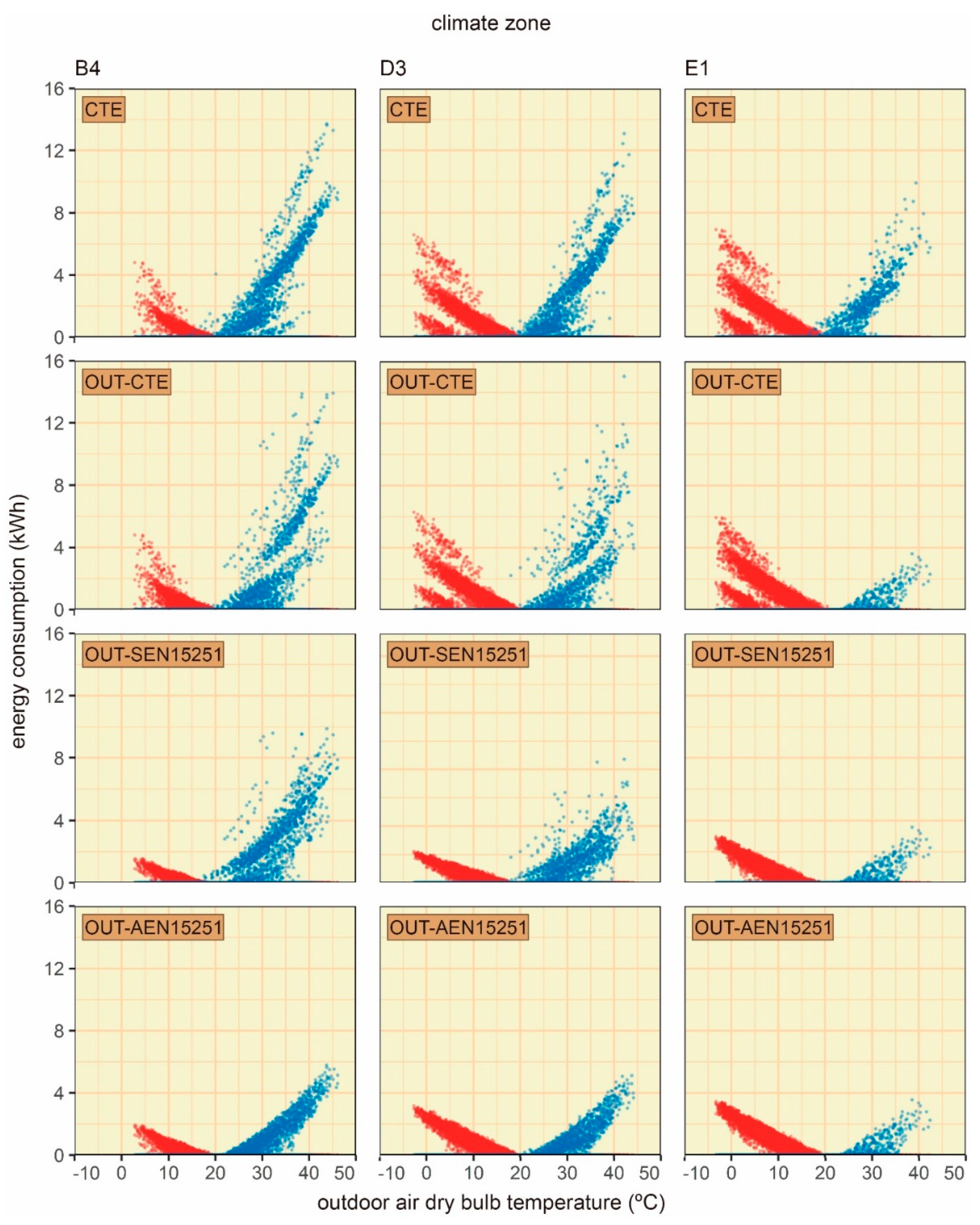
3.2. Influence of ACCIM on the Schedule Energy Consumption: Current Scenario

Figure 9 shows the hourly values of heating and cooling energy consumption. A different tendency between the static model and the adaptive models was found. In the analysis of the static model (CTE) of the three zones studied, B4 was the zone with the greatest summer climate severity. The highest pick of cooling consumption was, therefore, found in this zone by using such a model, reaching a schedule consumption of up to 11 kWh. In D3 and E1, the maximum cooling values oscillated between 7 and 4 kWh, although 10 and 7 kWh were reached in some hours. On the contrary, the highest heating consumption was produced in E1, exceeding 7 kWh.

The reduction of such maximum consumption values produced in the adaptive models in contrast to the CTE static model was analyzed. Considering that the consumptions between OUT-CTE, OUT-AEN15251, and OUT-SEN15251 were the same when the adaptive model was applied, the variations between the graphics sharing climate scenario and zone belonged to those hours when the static models were applied. As for CTE and OUT-CTE, those intermediate zones (in which there was no heating or cooling energy consumption) belonged to the change of the main and setback setpoint temperatures: (i) 20 °C and 17 °C for heating; and (ii) 27 °C and 25 °C for cooling.

Regarding the cooling energy consumption, there was a reduction in B4 in adaptive models with respect to the CTE model. In this way, the heating consumption had a similar behavior in this climate zone. For D3, the schedule values of heating and cooling were slightly lower than those of E1 and B4, respectively. However, Table 5 shows that the total consumption was equal or lower than that of E1, as well as higher than B4.

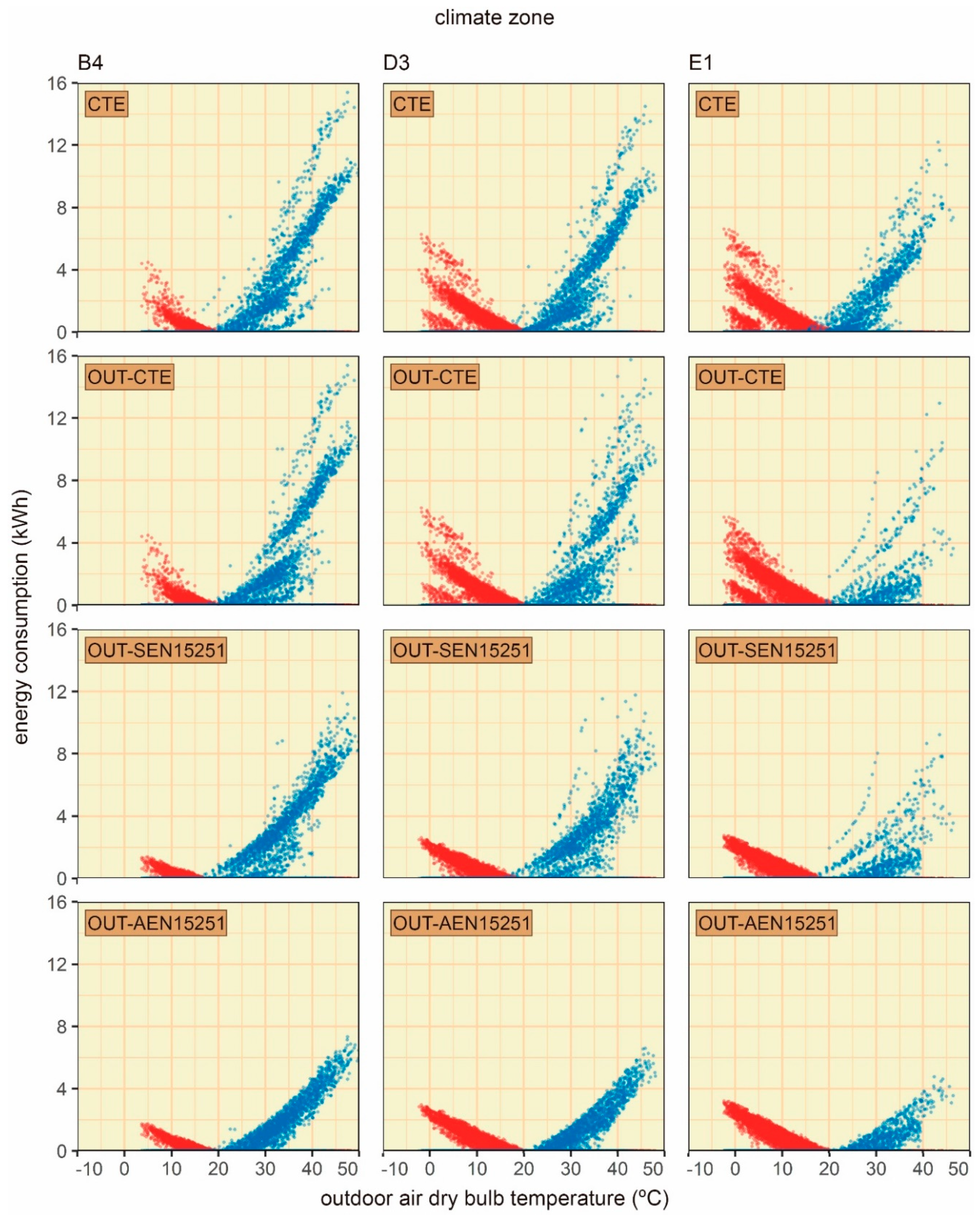
3.3. Influence of ACCIM on the Schedule Energy Consumption: Future Scenarios

To know the influence of climate change on comfort models, the analysis carried out in the current scenario was also conducted in future scenarios. Figure 10 and Figure 11 show the results of heating, cooling, and total energy consumption in 2050 and 2080 scenarios, respectively. Moreover,

Table 6. Consumption variability of the models according to the climate scenario.

Zone	Model		Scenario
			Current	2050		2080
			kWh/m2·Year	kWh/m2·Year	%	kWh/m2·Year	%
B4	CTE	Heating	1504.85	1060.49	−42%	687.07	−119%
		Cooling	3652.45	5196.55	30%	7116.07	49%
		Total	5157.30	6257.04	18%	7803.14	34%
	OUT-CTE	Heating	1484.04	1078.04	−38%	673.17	−120%
		Cooling	1682.26	3904.71	57%	6351.04	74%
		Total	3166.30	4982.75	36%	7024.22	55%
	OUT-SEN15251	Heating	1040.56	695.50	−50%	385.79	−170%
		Cooling	1561.01	3626.22	57%	5962.58	74%
		Total	2601.57	4321.72	40%	6348.36	59%
	OUT-AEN15251	Heating	1727.15	1220.57	−42%	759.12	−128%
		Cooling	1065.81	2052.95	48%	3616.59	71%
		Total	2792.96	3273.52	15%	4375.71	36%
D3	CTE	Heating	5105.23	4273.92	−19%	3368.92	−52%
		Cooling	2773.06	4150.70	33%	5931.86	53%
		Total	7878.28	8424.62	6%	9300.78	15%
	OUT-CTE	Heating	5113.53	4260.92	−20%	3371.96	−52%
		Cooling	745.89	2595.82	71%	4762.16	84%
		Total	5859.42	6856.73	15%	8134.12	28%
	OUT-SEN15251	Heating	4323.58	3556.26	−22%	2729.79	−58%
		Cooling	722.83	2395.47	70%	4448.74	84%
		Total	5046.41	5951.73	15%	7178.54	30%
	OUT-AEN15251	Heating	5778.52	4851.81	−19%	3835.79	−51%
		Cooling	640.52	1399.97	54%	2624.20	76%
		Total	6419.04	6251.78	−3%	6459.99	1%
E1	CTE	Heating	7005.40	6010.11	−17%	4863.72	−44%
		Cooling	844.63	1738.24	51%	3046.99	72%
		Total	7850.02	7748.36	−1%	7910.71	1%
	OUT-CTE	Heating	7037.78	6038.63	−17%	4876.70	−44%
		Cooling	37.54	229.21	84%	1174.32	97%
		Total	7075.32	6267.84	−13%	6051.02	−17%
	OUT-SEN15251	Heating	6079.29	5159.90	−18%	4117.06	−48%
		Cooling	37.72	228.41	83%	1090.36	97%
		Total	6117.01	5388.31	−14%	5207.42	−17%
	OUT-AEN15251	Heating	7864.73	6785.03	−16%	5510.47	−43%
		Cooling	37.72	228.41	83%	742.19	95%
		Total	7902.45	7013.44	−13%	6252.65	−26%

shows the percentages of increase and decrease by using the current scenario of each model as a reference, and the positive and negative values indicate the increase and the decrease, respectively.

In 2050 and 2080 scenarios, there were increases and decreases of the total consumption according to the climate zone: in B4, there were only increases because of high temperatures, whereas there were also increases in D3, albeit lower than those in B4. As for the OUT-AEN15251 model for 2050, there was a total decrease caused maybe by the high setpoint temperatures of such a model, which limited the increase of cooling consumption, thus compensating for the heating consumption. Also, there were decreases in E1, mainly because the variation of heating was greater than that of cooling. As for the CTE model in 2080, there was an increase because of the restrictive cooling setpoint temperature of 25 °C in daytime hours, which, together with the increase in temperature, implied a higher variation in cooling than in heating.

Regarding the maximum schedule consumption values in 2050 (Figure 10), the cooling decreased in B4 from 14 kWh in CTE and OUT-CTE to around 6 kWh in OUT-AEN15251. Moreover, heating decreased from values around 9 kWh in CTE to 3 kWh in OUT-SEN15251 and OUT-AEN15251.

Such values varied in 2080 (Figure 11), as for the cooling consumption in B4, from 16 kWh in CTE and OUT-CTE to around 7 kWh in OUT-AEN15251. As for the heating consumption in E1, values varied from around 7 kWh in CTE to 3 kWh in OUT-SEN15251 and OUT-AEN15251.

As for D3, in 2050 and 2080 scenarios, as well as in all comfort models, the maximum values of heating and cooling consumption were slightly lower than the heating values in E1 and the cooling values in B4. In this sense, the highest consumptions were achieved in this zone, except in the total consumption of the OUT-AEN15251 model in 2050, which was slightly lower than that in E1, maybe because of the high heating setpoints of the OUT-AEN15251 model, together with the low temperatures in E1.

4. Conclusions

This research suggests HVAC systems can be widely used by considering various adaptive comfort models. The adaptive comfort models depend on the external temperature; thus, their applicability range is limited. For this reason, to implement the so-called Adaptive Comfort Control Implemented Model (ACCIM), three different operation hypotheses were developed as possible approximations to the average weighted external temperatures outside the applicability ranges of the model. Thus, the approaches of OUT-CTE, OUT-SEN15251, and OUT-AEN15251 were compared with the current normative in force in Spain (CTE) and tested in three different zones of the national territory according to their climates (B4, D3, and E1) for their current scenario and their projections due to climate change in 2050 and 2080.

The results demonstrate that the consumption is reduced in different ways by using this predictive model, depending on the climate and the hypothesis selected. This variability is also detected in future projections (2050 and 2080). Generally, the OUT-SEN15251 and OUT-AEN15251 models presented the best performance in all climate zones, with the OUT-SEN15251 model obtaining the best behavior in most of the cases studied for the current scenario. Regarding future scenarios, the models with the best performance varied depending on the climate zone: for the warmest zones (B4), the model with the best performance was OUT-AEN15251; for the coldest climates (E1), the OUT-SEN15251 had the best performance; and the model which obtained the lowest consumption for mild climates (D3) in the current scenario and 2050 was OUT-SEN15251, whereas, in 2080, it was OUT-AEN15251.

Nevertheless, although there was a general increase in energy consumption due to global warming (more perceptible in the warmest zones), all the operation hypotheses of the ACCIM models were more resilient than those of the CTE, even recording total values of consumption which were lower in 2080 with respect to the static model in the CTE.

It must be understood that there was some margin of uncertainty in the simulation results. This was mainly due to the lack of information regarding future thermal comfort standards, future predictions on human behavior, and future predictions on the improvement of the energy performance of HVAC systems.

The results obtained in this research provide relevant information to reduce the energy consumption in buildings. The use of comfort models with adaptive setpoint temperatures significantly reduces the energy consumption in the existing buildings, both in current and future scenarios. Thus, the comfort model for the setpoint temperatures used by the normative in force in Spain has limitations to guarantee an acceptable performance of the existing building stock without damaging users’ life quality. This aspect is also shown in the normatives of other countries, in which the use of static setpoint temperatures is required. The results of this paper can, therefore, be extrapolated to other countries. Despite this, the applicability of such adaptive models to real case studies constitutes an aspect to be studied; thus, it should be analyzed in further research works.

Finally, more research studies in this field are required to carry out the transition of the static comfort models to models which are more related to the external climate conditions and which consider the users’ climate adaptation. In addition, these research works could support the transition of the Spanish normative to a more sustainable energy consumption without damaging people’s quality of life.

References

1. World Wildlife Fund. Living Planet Report 2014: Species and Spaces, People and Places; WWF International: Gland, Switzerland, 2014; Volume 1, ISBN 9780874216561. [Google Scholar]
2. European Commission. A Roadmap for Moving to a Competitive Low Carbon Economy in 2050; European Commission: Brussels, Belgium, 2011; pp. 1–15. [Google Scholar]
3. The United Nations Environment Programme. Building Design and Construction: Forging Resource Efficiency and Sustainable; The United Nations Environment Programme: Nairobi, Kenya, 2012. [Google Scholar]
4. Pérez-Lombard, L.; Ortiz, J.; Pout, C. A review on buildings energy consumption information. Energy Build. 2008, 40, 394–398. [Google Scholar] [CrossRef]
5. European Commission. Directive 2002/91/EC of the European Parliament and of the council of 16 December 2002 on the energy performance of buildings. Off. J. Eur. Union 2002, 65–71. [Google Scholar] [CrossRef]
6. European Union. Directive 2010/31/EU of the European Parliament and of the Council of 19 May 2010 on the Energy Performance of Buildings; European Union: Brussels, Belgium, 2010; Volume 153, pp. 13–35. [Google Scholar]
7. Horne, R.; Hayles, C. Towards global benchmarking for sustainable homes: An international comparison of the energy performance of housing. J. Hous. Built Environ. 2008, 23, 119–130. [Google Scholar] [CrossRef]
8. Kurtz, F.; Monzón, M.; López-Mesa, B. Energy and acoustics related obsolescence of social housing of Spain’s post-war in less favoured urban areas. The case of Zaragoza. Inf. La Construcción 2015, 67, m021. [Google Scholar] [CrossRef]
9. Lowe, R. Technical options and strategies for decarbonizing UK housing. Build. Res. Inf. 2007, 35, 412–425. [Google Scholar] [CrossRef] [Green Version]
10. Park, K.; Kim, M. Energy Demand Reduction in the Residential Building Sector: A Case Study of Korea. Energies 2017, 10, 1506. [Google Scholar] [CrossRef]
11. Page, J.; Robinson, D.; Morel, N.; Scartezzini, J.L. A generalised stochastic model for the simulation of occupant presence. Energy Build. 2008, 40, 83–98. [Google Scholar] [CrossRef]
12. Spanish Institute of Statistics Population and Housing Census. Available online: https://www.ine.es/censos2011_datos/cen11_datos_resultados.htm# (accessed on 9 November 2018).
13. Di Pilla, L.; Desogus, G.; Mura, S.; Ricciu, R.; Di Francesco, M. Optimizing the distribution of Italian building energy retrofit incentives with Linear Programming. Energy Build. 2016, 112, 21–27. [Google Scholar] [CrossRef]
14. Theodoridou, I.; Papadopoulos, A.M.; Hegger, M. A typological classification of the Greek residential building stock. Energy Build. 2011, 43, 2779–2787. [Google Scholar] [CrossRef]
15. Pérez-Andreu, V.; Aparicio-Fernández, C.; Martínez-Ibernón, A.; Vivancos, J.L. Impact of climate change on heating and cooling energy demand in a residential building in a Mediterranean climate. Energy 2018, 165, 63–74. [Google Scholar] [CrossRef]
16. Bienvenido-Huertas, D.; Quiñones, J.A.F.; Moyano, J.; Rodríguez-Jiménez, C.E. Patents Analysis of Thermal Bridges in Slab Fronts and Their Effect on Energy Demand. Energies 2018, 11, 2222. [Google Scholar] [CrossRef]
17. Isaac, M.; van Vuuren, D.P. Modeling global residential sector energy demand for heating and air conditioning in the context of climate change. Energy Policy 2009, 37, 507–521. [Google Scholar] [CrossRef]
18. Cellura, M.; Guarino, F.; Longo, S.; Tumminia, G. Climate change and the building sector: Modelling and energy implications to an office building in southern Europe. Energy Sustain. Dev. 2018, 45, 46–65. [Google Scholar] [CrossRef]
19. Intergovernmental Panel on Climate Change Climate change 2014: Synthesis report. Contribution of working groups I, II and III to the fifth assessment report of the intergovernmental Panel on climate change. In Climate Change 2013—The Physical Science Basis; Intergovernmental Panel on Climate Change (Ed.) Cambridge University Press: Cambridge, UK, 2014; pp. 1–30. [Google Scholar]
20. Karimpour, M.; Belusko, M.; Xing, K.; Boland, J.; Bruno, F. Impact of climate change on the design of energy efficient residential building envelopes. Energy Build. 2015, 87, 142–154. [Google Scholar] [CrossRef]
21. Kalvelage, K.; Passe, U.; Rabideau, S.; Takle, E.S. Changing climate: The effects on energy demand and human comfort. Energy Build. 2014, 76, 373–380. [Google Scholar] [CrossRef]
22. Rubio-Bellido, C.; Perez-Fargallo, A.; Pulido-Arcas, J.A. Optimization of annual energy demand in office buildings under the influence of climate change in Chile. Energy 2016, 114, 569–585. [Google Scholar] [CrossRef]
23. Roaf, S.; Crichton, D.; Nicol, F. Adapting Buildings and Cities for Climate Change: A 21st Century Survival Guide; Routledge: London, UK, 2009. [Google Scholar]
24. Ren, Z.; Chen, D. Modelling study of the impact of thermal comfort criteria on housing energy use in Australia. Appl. Energy 2018, 210, 152–166. [Google Scholar] [CrossRef]
25. Tushar, W.; Wang, T.; Lan, L.; Xu, Y.; Withanage, C.; Yuen, C.; Wood, K.L. Policy design for controlling set-point temperature of ACs in shared spaces of buildings. Energy Build. 2017, 134, 105–114. [Google Scholar] [CrossRef] [Green Version]
26. Hoyt, T.; Arens, E.; Zhang, H. Extending air temperature setpoints: Simulated energy savings and design considerations for new and retrofit buildings. Build. Environ. 2014, 88, 89–96. [Google Scholar] [CrossRef]
27. Wan, K.K.W.; Li, D.H.W.; Lam, J.C. Assessment of climate change impact on building energy use and mitigation measures in subtropical climates. Energy 2011, 36, 1404–1414. [Google Scholar] [CrossRef]
28. Parry, M.L.; Canziani, O.F.; Palutikof, J.P.; van der Linden, P.J.; Hanson, C.E. Contribution of Working Group II to the Fourth Assessment Report of the Intergovernmental Panel on Climate Change; Cambridge University Press: Cambridge, UK, 2007. [Google Scholar]
29. Spyropoulos, G.N.; Balaras, C.A. Energy consumption and the potential of energy savings in Hellenic office buildings used as bank branches—A case study. Energy Build. 2011, 43, 770–778. [Google Scholar] [CrossRef]
30. Bienvenido-Huertas, D.; Rubio-Bellido, C.; Pérez-Ordóñez, J.; Martínez-Abella, F. Estimating Adaptive Setpoint Temperatures Using Weather Stations. Energies 2019, 12, 1197. [Google Scholar] [CrossRef]
31. Pérez-Fargallo, A.; Pulido-Arcas, J.A.; Rubio-Bellido, C.; Trebilcock, M.; Piderit, B.; Attia, S. Development of a new adaptive comfort model for low income housing in the central-south of chile. Energy Build. 2018, 178, 94–106. [Google Scholar] [CrossRef]
32. Sánchez-García, D.; Rubio-Bellido, C.; Pulido-Arcas, J.A.; Guevara-García, F.J.; Canivell, J. Adaptive comfort models applied to existing Dwellings in Mediterranean climate considering globalwarming. Sustainability 2018, 10, 3507. [Google Scholar] [CrossRef]
33. van der Linden, A.C.; Boerstra, A.C.; Raue, A.K.; Kurvers, S.R.; De Dear, R.J. Adaptive temperature limits: A new guideline in the Netherlands: A new approach for the assessment of building performance with respect to thermal indoor climate. Energy Build. 2006, 38, 8–17. [Google Scholar] [CrossRef]
34. Boerstra, A.C.; van Hoof, J.; van Weele, A.M. A new hybrid thermal comfort guideline for the Netherlands: Background and development. Arch. Sci. Rev. 2015, 58, 24–34. [Google Scholar] [CrossRef]
35. Kramer, R.; van Schijndel, J.; Schellen, H. Dynamic setpoint control for museum indoor climate conditioning integrating collection and comfort requirements: Development and energy impact for Europe. Build. Environ. 2017. [Google Scholar] [CrossRef]
36. American National Standards Institute/American Society of Heating Refrigerating and Air-Conditioning Engineers (ANSI/ASHRAE). ANSI/ASHRAE Standard 55-2013: Thermal Environmental Conditions for Human Occupancy; ASHRAE: Atlanta, GA, USA, 2013. [Google Scholar]
37. Sánchez-Guevara Sánchez, C.; Mavrogianni, A.; Neila González, F.J. On the minimal thermal habitability conditions in low income dwellings in Spain for a new definition of fuel poverty. Build. Environ. 2017, 114, 344–356. [Google Scholar] [CrossRef] [Green Version]
38. Barbadilla-Martín, E.; Salmerón Lissén, J.M.; Martín, J.G.; Aparicio-Ruiz, P.; Brotas, L. Field study on adaptive thermal comfort in mixed mode office buildings in southwestern area of Spain. Build. Environ. 2017, 123. [Google Scholar] [CrossRef]
39. Barbadilla-Martín, E.; Guadix Martín, J.; Salmerón Lissén, J.M.; Sánchez Ramos, J.; Álvarez Domínguez, S. Assessment of thermal comfort and energy savings in a field study on adaptive comfort with application for mixed mode offices. Submitt. Energy Build. 2017. [Google Scholar] [CrossRef]
40. European Committee for Standardization. EN 15251: Indoor Environmental Input Parameters for Design and Assessment of Energy Performance of Buildings—Addressing Indoor Air Quality, Thermal Environment, Lighting and Acoustics; CEN: Brussels, Belgium, 2007; Volume 3, pp. 1–52. [Google Scholar]
41. Sánchez-García, D.; Rubio-Bellido, C.; del Río, J.J.M.; Pérez-Fargallo, A. Towards the quantification of energy demand and consumption through the adaptive comfort approach in mixed mode office buildings considering climate change. Energy Build. 2019, 187, 173–185. [Google Scholar] [CrossRef]
42. The Government of Spain. Royal Decree 314/2006. Approving the Spanish Technical Building Code CTE-DB-HE-1; The Government of Spain: Madrid, Spain, 2013.
43. Naspi, F.; Arnesano, M.; Stazi, F.; D’Orazio, M.; Revel, G.M. Measuring Occupants’ Behaviour for Buildings’ Dynamic Cosimulation. J. Sens. 2018, 2018, 1–17. [Google Scholar] [CrossRef]
44. Castaño-Rosa, R.; Solís-Guzmán, J.; Marrero, M. A novel Index of Vulnerable Homes: Findings from application in Spain. Indoor Built Environ. 2018. [Google Scholar] [CrossRef]
45. The Government of Spain. Código Técnico de la Edificación Documento Básico HE Climas de Referencia; The Government of Spain: Madrid, Spain, 2015.
46. Rubel, F.; Kottek, M. Observed and projected climate shifts 1901–2100 depicted by world maps of the Köppen-Geiger climate classification. Meteorol. Z. 2010, 19, 135–141. [Google Scholar] [CrossRef]
47. American National Standards Institute/American Society of Heating Refrigerating and Air-Conditioning Engineers (ANSI/ASHRAE). ASHRAE Guideline 14-2014: Measurement of Energy, Demand, and Water Savings; ASHRAE: Atlanta, GA, USA, 2014; p. 146. [Google Scholar]
48. Bienvenido-Huertas, D.; Moyano, J.; Rodríguez-Jiménez, C.E.; Marín, D. Applying an artificial neural network to assess thermal transmittance in walls by means of the thermometric method. Appl. Energy 2019, 233–234, 1–14. [Google Scholar] [CrossRef]
49. Jentsch, M.F.; Bahaj, A.S.; James, P.A.B. Climate Change World Weather Gen, Climate Change World Weather File Generator, Version 1.8; Sustainable Energy Research Group: Southampton, UK, 2013. [Google Scholar]
Figure 1. Methodology flowchart.
Energies 12 01498 g001
Figure 2. Setpoints of Spanish Building Technical Code (CTE), OUT-CTE, OUT-SEN15251, and OUT-AEN15251 models.
Energies 12 01498 g002
Figure 3. Case study analyzed.
Energies 12 01498 g003
Figure 4. Constructive properties.
Energies 12 01498 g004
Figure 5. Operative schedules.
Energies 12 01498 g005
Figure 6. (a) Thermal model; (b) dwellings analyzed.
Energies 12 01498 g006
Figure 7. Evolution of climate conditions.
Energies 12 01498 g007
Figure 8. Global energy consumption for the different models and scenarios considered.
Energies 12 01498 g008
Figure 9. Relationship between hourly energy consumption and outdoor hourly temperature of the static model and adaptive models in current scenario.
Energies 12 01498 g009
Figure 10. Relationship between hourly energy consumption and outdoor hourly temperature of the static model and adaptive models in 2050.
Energies 12 01498 g010
Figure 11. Relationship between hourly energy consumption and outdoor hourly temperature of the static model and adaptive models in 2080.
Energies 12 01498 g011