1. Introduction
The need to reduce greenhouse gas emissions is ever increasing, and several nations have agreed on ambitious targets in the Paris Agreement Treaty [
1]. This treaty has the aim to limit global temperature 2 °C above the pre-industrial levels. The transportation and its infrastructure represents 23% of greenhouse gas emissions and is only surpassed by fossil fuel emissions (e.g., energy production) [
2]. This shows that the electrification of transport plays a significant role in making the planet a greener place, reducing dependence on fossil fuels.
The use of electric vehicles (EVs) not only has the potential to change individual mobility but also to reduce pollutant emissions, which is considered a major cause of air pollution and causes serious health problems in the global population. However, as an increasing number of charges will ideally be covered by renewable production to achieve decarbonization of the transportation sector, the introduction of dynamic electricity prices could increase the risk of substation overloads [
3]. In Europe, growth in the use of EVs will result in extra energy demand, with consumption increasing from approximately 0.03% in 2014 to 9.5% in 2050 [
4].
Generally, the population is accustomed to deal with fossil energies and with the convenience of easy to find service stations and fast refueling times. Thus, there are no concerns regarding waiting times or about the fuel needed to reach the intended destination. When using an electric vehicle it is essential to consider these factors as the current range of the vehicles is limited and changing stations are few. Also, there are other challenges such as increasing peak power demand if the charging events occur at the same instant as residential or industrial peak consumption [
5]. The electrical network reacts according to the level of loads connected to it, and with growing usage of this mean of transportation in the future, it is necessary to study how the impact of the extra energy required can be mitigated. Understanding the behavior of electric vehicle users while at the same time recognize the changes in the network will be a crucial part.
Recent studies suggest that dynamic electricity prices can spur demand and help electric companies avoid costly investments in infrastructures [
6]. However, the lack of variability in electricity prices does not allow the studies to be completely realistic or in line with the actual variability of renewable energy generation. In this context, it is crucial to address the following research question: can electric vehicle users change their charging patterns as a result of varying electricity prices?
Providing incentives to EV users in a way that behavior and charging patterns are changed and adapted accordingly to the variation of electricity prices is essential to ensure the EV’s flexibility balances the variation of renewable energy sources. It is in this scope that this paper brings its main contributions, by presenting a study on the impact of electricity prices variation on EV users’ charging habits.
This study compares the benefits when using a variable and fixed charging prices. The variable prices are determined based on the calculation of distribution locational marginal pricing (DLMP) using distribution network operation and reconfiguration optimization model, which enables achieving prices that are not only continuously recalculated and adaptable to the ongoing changes in the power network (variation of consumption and generation at each time) but also reflect the situation and needs in each different location of the network. These prices are used to incentive EV users to change their charging habits according to the variation of renewable generation in different places of the power network. A travel simulation tool specifically developed for this study is also presented. The simulator takes into account the behavior of real users to simulate their trips from the origin place (e.g., house or workplace) to multiple destinations, and back. The tool also considers different types of users and vehicles, thus allowing to create personalized profiles, destinations, and schedules. Moreover, the simulator enables defining the position of the vehicles in a power network continuously throughout time. In this way, the proposed tool simulates a real environment, with trips and charging stations (CS). Considering the defined scenarios, users make decisions regarding their charging process, i.e., if they charge their vehicles or not at each time, according to the behaviors previously analyzed. For this, intelligent charging is simulated considering variables such as distance and the price of electricity. In this way, it is possible to test the impact of different types of incentives on EV users’ behavior. A physical laboratory model of a smart city (SC) located at BISITE laboratory with a 13 buses distribution network with high distributed energy resources (DER) penetration is used to demonstrate the application of the proposed methodology. Results show that variable charging prices prove to be more advantageous to the EV users, enabling them to reduce charging costs, while contributing to the required flexibility for the system. This allows mitigating the problems introduced with the large-scale penetration of distributed, variable renewable energy sources.
The rest of the paper is organized as follows:
Section 2 presents a brief review of state of the art. The proposed simulator tool is described in
Section 3, along with the methodology for the calculation of the variable electricity prices. The case studies are discussed in
Section 4. Finally, the conclusions are shown in
Section 6.
2. State of the Art
2.1. Electric Mobility
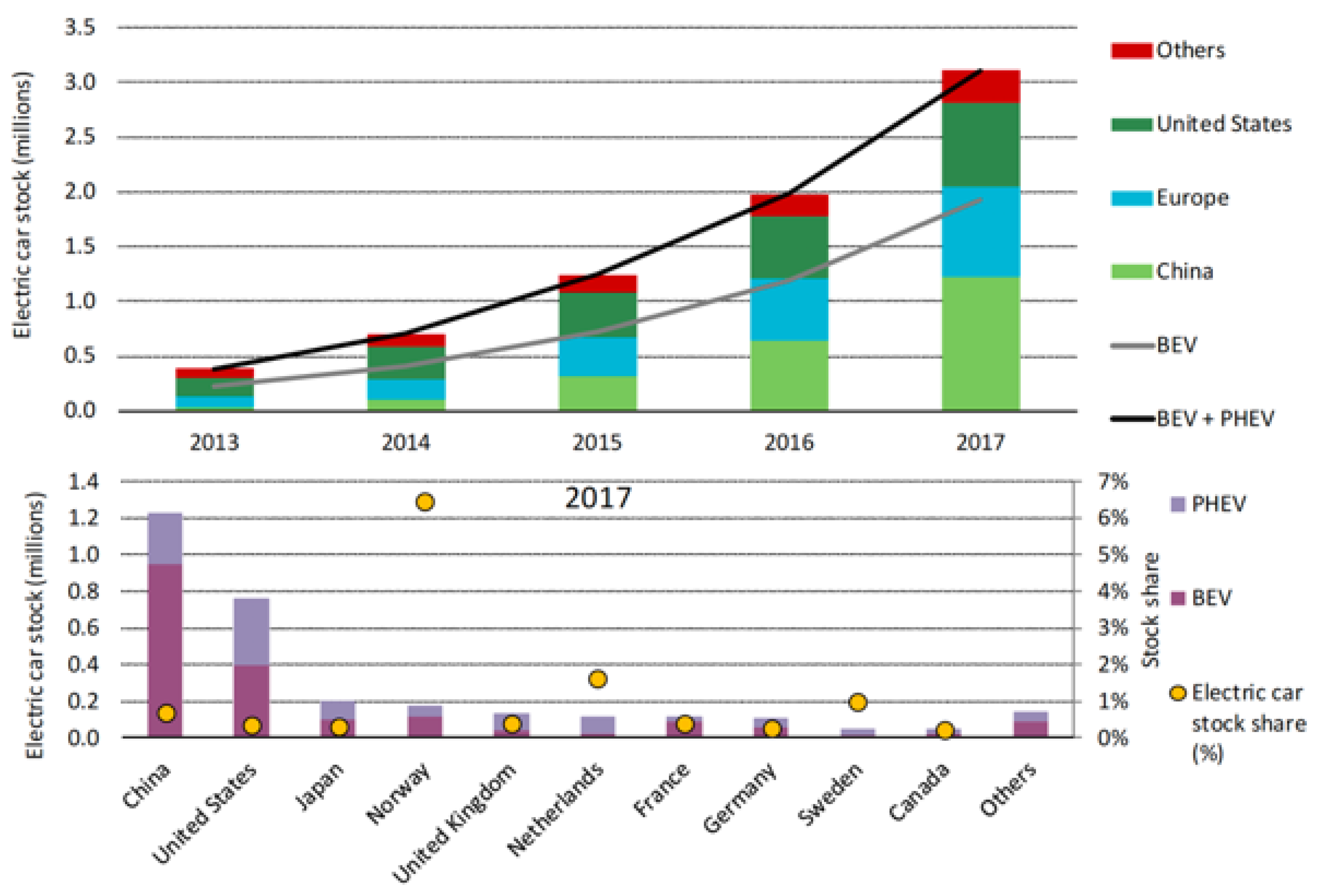
In 2017, the number of EVs on the road was about 3.1 million, an increase of 57% compared to 2016 (according to
Figure 1). This increase was similar to that registered between 2015 and 2016, of 60% [
7]. It is also possible to verify that purely electric vehicles (battery electric vehicle - BEV), had a more significant growth than the hybrid vehicles (plug-in hybrid electric vehicle - PHEV), representing two-thirds of the total. China is the country with the largest share, accounting for 40% of the total [
7].
With the increasing popularity of EVs, there is the need to improve charging infrastructures and offer more affordable models. While governments offer incentives for adopting EVs and continue to invest in infrastructure, the motive that drives people to opt for this type of transportation is socially driven: it is the cleanest solution that will help sustain a habitable planet. This is reflected in the satisfaction of EVs’ users, where 51% say that the most significant incentive to buy one is to contribute to a more sustainable future [
8].
Overall, the results show that this adoption does not only depend on incentives but also fewer obstacles to a more comfortable driving. In this sense, it is essential that charging is accessible, both monetarily and geographically. It is important to have homes, shopping malls, workplaces, and parking lot buildings with charging stations.
Another aspect to consider is the type of charging since time spent stopped is perhaps the variable that the consumer values most. The high power capacity of fast chargers (with a power greater than 40 kW) makes them difficult to implement in residential homes due to possible hazards, which even being addressed, are still mostly underdeveloped. To this, the implementation of fast CS will facilitate the user by reducing waiting times.
2.2. Charging Behaviour
Between 2011 and 2013 data about driving and EV demand patterns were collected on a study conducted in Europe [
9]. More than 230,000 charges have been registered. The average state of charge (SoC) of the battery was of 60% when users recharged it, which shows that users do not let the battery discharge completely and charge it whenever they have the opportunity and not when the battery is low. The average percentage of users who started a journey or a charge with a SoC level of less than 20% is less than 5%. Regarding the moment of the charging, it is verified that the majority are performed between 18:00 and 22:00, which corresponds to the peak hours of energy demand.
Franke and Krems [
10] analyzed the charging behavior of users in Germany. They concluded that the true vehicle range affects charging decisions. They have also developed a conceptual model based on principles of self-regulation and control theory where it is possible to understand the use of energy resources. This model is based on the premise that whenever users interact with limited power sources, they continuously monitor and manage their mobility needs and their mobility resources. For instance, the mobility needs relate to the distance of a trip and the mobility resources relate to the remaining battery. Users often feel "range anxiety" that can be described as the experience of never having enough battery to reach a location and getting stranded. Thus, as the anxiety increases so does the likelihood of resorting to strategies to handle this situation, e.g., driving economically or charging the car more often.
Marmaras et al. [
11] developed two behavioral profiles to be used in a simulation environment: unaware and aware. The unaware profile tries to find the best possible solution with limited access to information and minimal interaction with the environment and other EVs’ users. In this case, the level of range anxiety is strong, and the user is always seeking to charge the vehicle even when it is not needed. The aware profile has more access to information and interacts with the environment and other EVs. This profile has a low anxiety level, charging the vehicle only when needed. The results of this research show that the unaware profile starts charging the vehicle as soon as it is parked, typically at home between 17:30 and 18:00, whereas the aware profile waits for the off-peak hours between 22:00 and 06:00 h.
Neubauer and Wood [
12] applied a battery life analysis and simulation tool for vehicles (BLAST-V) of the National Renewable Energy Laboratory to study the sensitivity of EVs concerning range anxiety and different scenarios of different charging infrastructures. The results showed that the effects of range anxiety might be significant but reduced with access to additional charging infrastructures.
Nicholas et al. [
13] studied the charging behavior when simulating trips and charging in public stations. The results show that more than 5% of trips would require recharging in a public charger for different charging autonomy and assumptions.
Xu et al. [
14] used a mixed logic model to study which factors influence BEV users in the decision-making of the type of charging (normal or fast) and local. The results suggest that the battery capacity, the initial state of the battery and the number of fast charges carried out are the predictive factors for the choice of type and place of charging of the users. Also, the day range between the current and next trip positively affects normal charging at home/business.
2.3. Distribution Locational Marginal Pricing
The distribution network congestion may occur, with the high penetration level of EVs. However, the congestion problems can be handled by the distribution system operator (DSO) with the employment of market-based congestion control methods [
15]. The way how locational marginal pricing (LMP) in transmission systems are obtained can be extended to the distribution systems [
16], usually named as distribution locational marginal pricing (DLMP). It is known that the resistance of the distribution network lines is higher than that of transmission lines. Thus, the distribution system losses can be considered one of the main factors that affect the DLMP [
17]. To deal with the EV demand congestion in distribution networks, Reference [
18] proposes step-wise congestion management developed whereby the DSO predicts congestion for the next day and publishes day-ahead tariff before the clearing of the day-ahead market. Reference [
19] solves the social welfare optimization of the distribution system considering EV aggregators as price takers in the local DSO market and demand price elasticity. Reference [
20] presents a market-based mechanism using the DLMP concept to alleviate possible distribution system congestion due to EVs and heat pump integration. Additional, Reference [
21] propose a DLMP-based algorithm with quadratic programming to deal with the congestion in distribution networks with high penetration of EVs and heat pumps.
2.4. Simulation Tools
SUMO (Simulation of Urban MObility) [
22] is perhaps the best-known traffic simulator. It is an intermodal and multimodal traffic flow simulation platform, which includes vehicles, public transportation, and pedestrians. SUMO has several tools that allow it to perform tasks such as locating routes, importing networks and calculating emissions. It can be enhanced with custom templates and provides multiple application programming interfaces (API) to control the simulation remotely.
MatSim [
23] is a framework for large-scale, agent-based simulations. Each agent has a transport demand represented by a chain of activities that must be done in a day at different times and locations. Decisions on how to travel between places are planned before the simulation. [
24] presents a method for the synthesis and animation of realistic traffic flows in large-scale road networks. It uses a technique based on a model of continuous traffic flow. Other multi-agent models are often used to create drivers behavior models.
When incorporating EVs into the simulation aspects such as power consumption, charging stations available and the charging duration must be considered [
25]. The problem of the shortest path and travel planning is studied in [
26], where the authors designed an approximation scheme to calculate the most energy-efficient path. In [
27] it is possible to do traffic simulations using only electric vehicles, where EVs are simulated on roads with online charging. A similar case is that of [
28], in which a spatial and temporal model was constructed to charge EVs in highway public chargers. Soares et al. [
29] presents a probabilistic simulator that generates driving and charging profiles of EVs that can be customized to adapt to different distribution networks. It simulates how vehicles move to estimate the impacts that charging may have on each configuration of the system, the energy consumed or emissions.
There are also other simulation tools related to EVs. FASTSim [
30] is a simulation tool that compares vehicles powertrain and estimates the impact of technological improvements to vehicle efficiency, performance, cost, and battery life. V2G-Sim uses individual driving and charging models of EVs to generate spatial and temporal impact/opportunity provisions in the electric grid [
31]. Alegre et al. [
32] proposes a pure and hybrid EV model, using a Matlab/Simulink environment, focusing on different aspects of the vehicle such as engine power, battery, and observing how the distance traveled and performance can be affected by the changes of the vehicles’ features.
Table 1 presents a summary of the main characteristics of the reviewed tools. It shows that the reviewed simulation tools share some limitations, such as the lack of charging decisions using learned to charge behaviors, and missing variable prices. Our proposed model overcomes both these limitations, by incorporating dynamic adaptation of charging behaviors from EV users, and the application of variable charging prices in the simulation model. Moreover, the proposed model includes several components also considered by other simulators, such as the simulation and analysis of trips, and the modeling and analysis of charging stations. The proposed model only partially considers the electrical network distribution impact of the EV user decisions. The effect of changes in demand and generation throughout the time of the electricity prices is considered using the DLMP-based distribution network operation and reconfiguration optimization model. The aim is to overcome several limitations in the current state-of-the-art developments.
3. Proposed Simulation Tool
In this section, the simulation tool parameters and algorithm are described. The tool allows the simulation of electric vehicle trips in a simple way, and it was developed using
R language using
RStudio integrated development environment [
33].
3.1. Parameters
The global parameters of the simulator are described in
Table 2. These parameters mean that they are applied to all the generated profiles, i.e., for any moment of the simulation they are the same. These are default values but can be changed according to user preferences.
3.2. Simulator Algorithm
The simulator consists of two main parts: data generation and simulation of trips. Data is generated concerning the profile of each user, such as vehicle features (battery, consumption, etc.), trips to be performed (locations and departure times) and behavioral parameters.
3.3. Data Generation
Population generation is an iterative process in which each of the variables is generated randomly from a sample of values with individual probabilities. Initially, each profile is assigned an initial location, depending on the available positions in the city map. This location will be a residence or a point of exit/entry into the city, considering users that live the city. Values are generated for the initial SoC, the preferred charging level, and the travel profile. It also generated the value of the battery capacity that will determine the rest of the characteristics of the vehicle. In the same way, a weight is assigned for the distance in terms of the charging station choosing, being the remaining weights attributed according to this value. The last data sets to be generated are the trips and times as well as their importance. Algorithm 1 has the following structure:
| Algorithm 1 Data generation algorithm. |
- 1:
for each of the cars do - 2:
Add an x coordinate to variable x - 3:
if x equal to some of the correspondent existent x available on the map then - 4:
Add y coordinate to y variable - 5:
end if - 6:
Generate initial SoC, available range preference, battery capacity and trip importance - 7:
Random generate w1 - 8:
if w1 equals to a specific value then - 9:
w2 = 1-w1-w3 - 10:
w3 = 1-w1-w2 - 11:
end if - 12:
if cars battery = value then - 13:
Attribute all data to this car model in the cars data frame - 14:
end if - 15:
for i:=0 to 5 do - 16:
Number of trips = 2, 3, 4 or 10-15 - 17:
Generate trips importance - 18:
Generate locations for the number of trips - 19:
Generate work day times, night times and/or leisure times - 20:
end for - 21:
end for
|
3.4. Trip Simulation
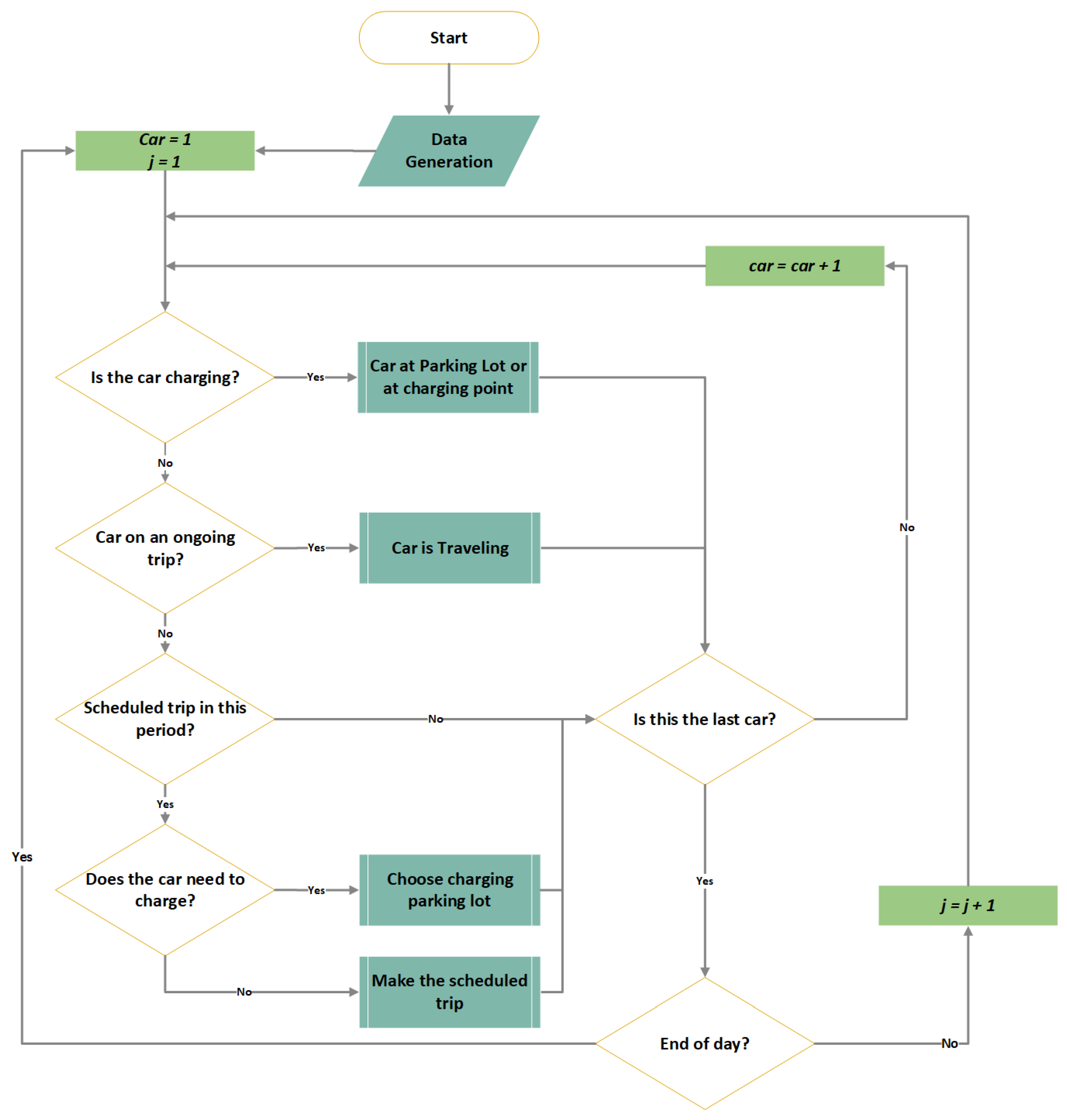
The trips simulation runs in periods of 15 min, totalling to 96 (
j = 96) for a full day. Its entire structure and mode of operation are described through a flow chart in
Figure 2. Each vehicle has an initial location and a series of trips to be performed during the day. Each trip has a departure time, the period
j in which the user will make that trip. When this happens, the Euclidean distance is calculated between the start location and the end location, with a margin of 20%, since the calculated distance is straight, and then it is multiplied by the scaling factor
. Knowing the distance, the travel time is determined according to the average speed of the vehicle. For instance, if the calculated distance is 9000 m, and the average speed is 35 km/h, the travel time will be 15 min and 26 s, which is longer than one interval, and thus it will consume two periods. However, if the average speed is 40 km/h, the travel time will be 13 min and 30 s, which is equivalent to one period. The following equation determines the travel time:
where:
3.5. Charging Stations
To simulate charging, four public charging stations (parking lot buildings) were created along with domestic chargers. Of the public stations, two are a slow charge (of 7.2 kW), and two are a fast charge (of 50 kW). The domestic chargers have a power of 3.7 kW.
The location of the stations was not chosen following a specific methodology. Their distribution covered all points of the city, with some randomness. In this sense, the objective is to understand what and how the various factors can influence the choice of charging sites and how energy prices influence EV users behavior.
3.6. Charging Decisions
When the user decides to charge the EV, a location must be chosen (a charging station or house). For this simulation, three variables were considered: distance, energy price and charging time (slow or fast). After determining the scores of each of those variables and considering the preferences of each user, it is obtained the final score (Equation (
2)). The charging station with the highest score is the one chosen to charge the vehicle.
where:
—Distance score from 0 to 100
—Price score from 0 to 100
—Charge time score from 0 to 100
w—Weight for each of the variables ( for distance preference; for price preference; for time preference)
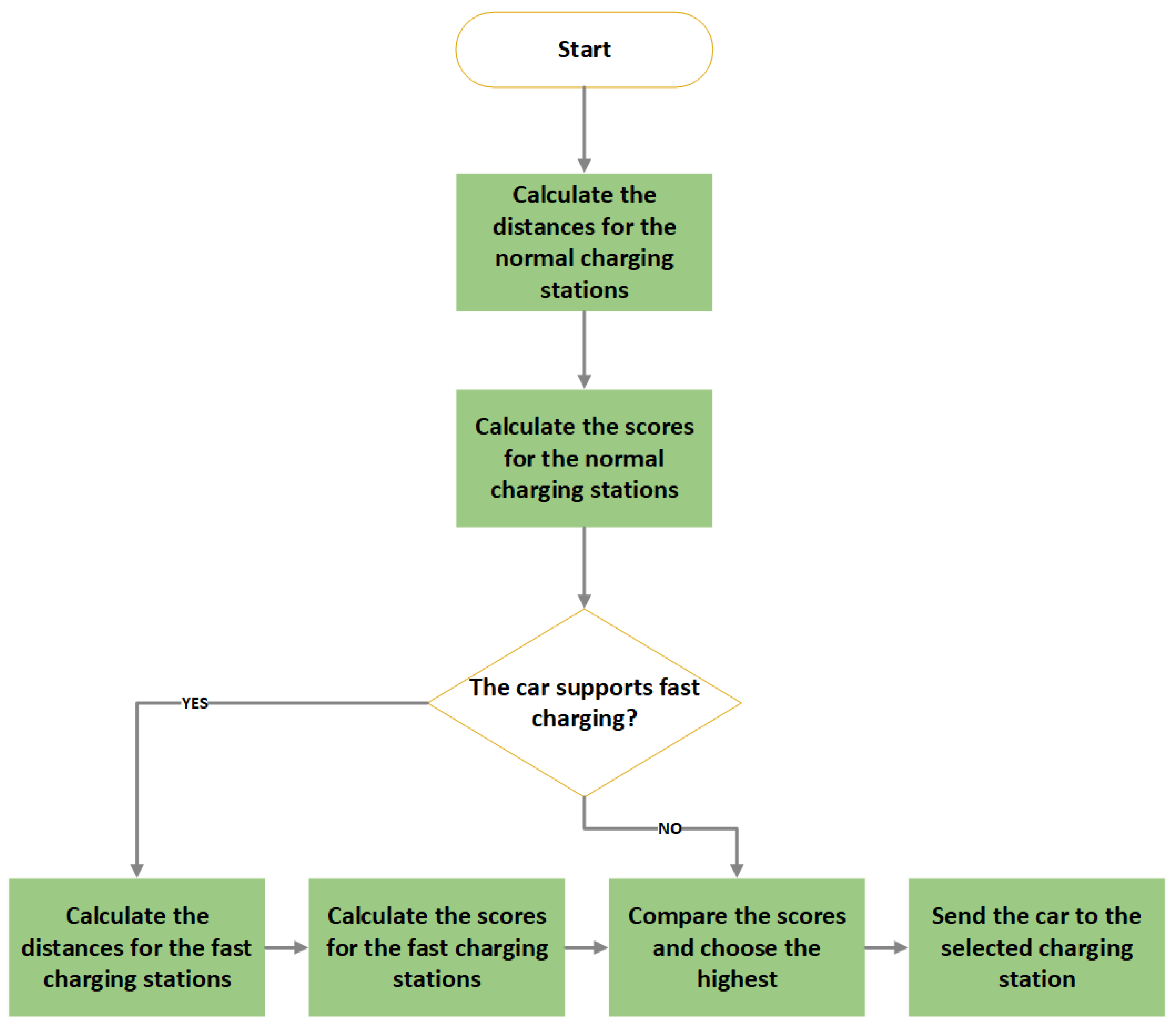
The process of selecting the preferred place to charge follows the structure described in
Figure 3. The distances to slow charging stations are calculated. These values, together with the energy price (€/kWh) and the charging time that the user has, allows a final score between 0 and 100 for each station. If the vehicle allows fast charging, this process is repeated for these types of charging stations. Finally, the scores of the charging stations are compared, and the highest is chosen.
To determine how long each user can delay or not a trip to charge his vehicle a variable was introduced that defines its importance. Thus, three different levels were assigned:
Low importance: this trip is discarded, and the car is charged until the next trip;
Medium importance: the user delays the trip, and all subsequent ones, until a time limit that varies according to the user profile;
High importance: the user must carry out this trip, not being able to charge, unless the level of battery charge reaches critical values.
To ensure that each user always has sufficient charge to make the trips, it was considered a critical battery level. Following the results of [
9] this value is set to 20%. Whenever a user reaches a level lower than this, regardless of the trip, the car must be charged. In this case, there are two options: either the user finds a place near the workplace (1st destination) and leaves the car there until the next trip, or looks for the nearest parking place and leave it there overnight until the next scheduled trip. It is assumed that the user leaves the car at this location and, hypothetically, does the rest of its travel using another mean of transportation.
3.7. Energy Prices
One of the variables that the users consider when deciding where to charge their vehicle is the energy price. This price differs between the type of station (slow or fast) and if they are public or domestic. Also, there are two domains where prices differ: fixed prices or variable prices.
In terms of simulation, in the case of fixed prices the user always pays the same regardless of the charging time. The only difference is whether it is a fast charging station or a domestic one, as a fast charging station is more costly. The variable prices vary by 15-min intervals. This is accomplished using the model described in
Section 2.3. Firstly, an additional cost which is related to the fixed term of network price rate to be charged to the customer (Equation (
3)) is calculated:
where:
Then the final energy price for the consumer is calculated (Equation (
4)). This value is the sum of the DLMP received, with the energy tariff and the additional price previously calculated (Equation (
3)). To Equation (
4) a fee of 5% is added by the owner of the charging station and the VAT value.
where:
—Distribution locational marginal pricing [€/kWh]
—Energy tariff price for each period [€/kWh]
—Additional profit margin of the parking owner
—Value added tax
3.8. DLMP Optimisation Model Description
In this research work, the DLMPs (which will permit to determine the variable charging price (see Equation (
4))) are defined through Lagrangian multipliers of the corresponding constraints (power balance) of the optimisation problem which has the goal to minimise the DSO expenditures [
34]. Thus, the DSO seeks to:
Minimize the power losses cost;
Minimize the power not supplied cost;
Minimize the power lines congestion cost;
Minimize the power generation curtailment cost;
Minimize the power from external suppliers cost.
The DLMPs optimization problem is classified as mixed-integer nonlinear programming (MINLP) due to the non-linearity features. To solve complex problems like this, Benders decomposition is an adequate technique [
35,
36]. The following constraints are considered:
4. Case Studies
To carry out the case studies a physical model of SC by GECAD-BISITE [
34] was used. The considered SC presents five types of loads, namely:
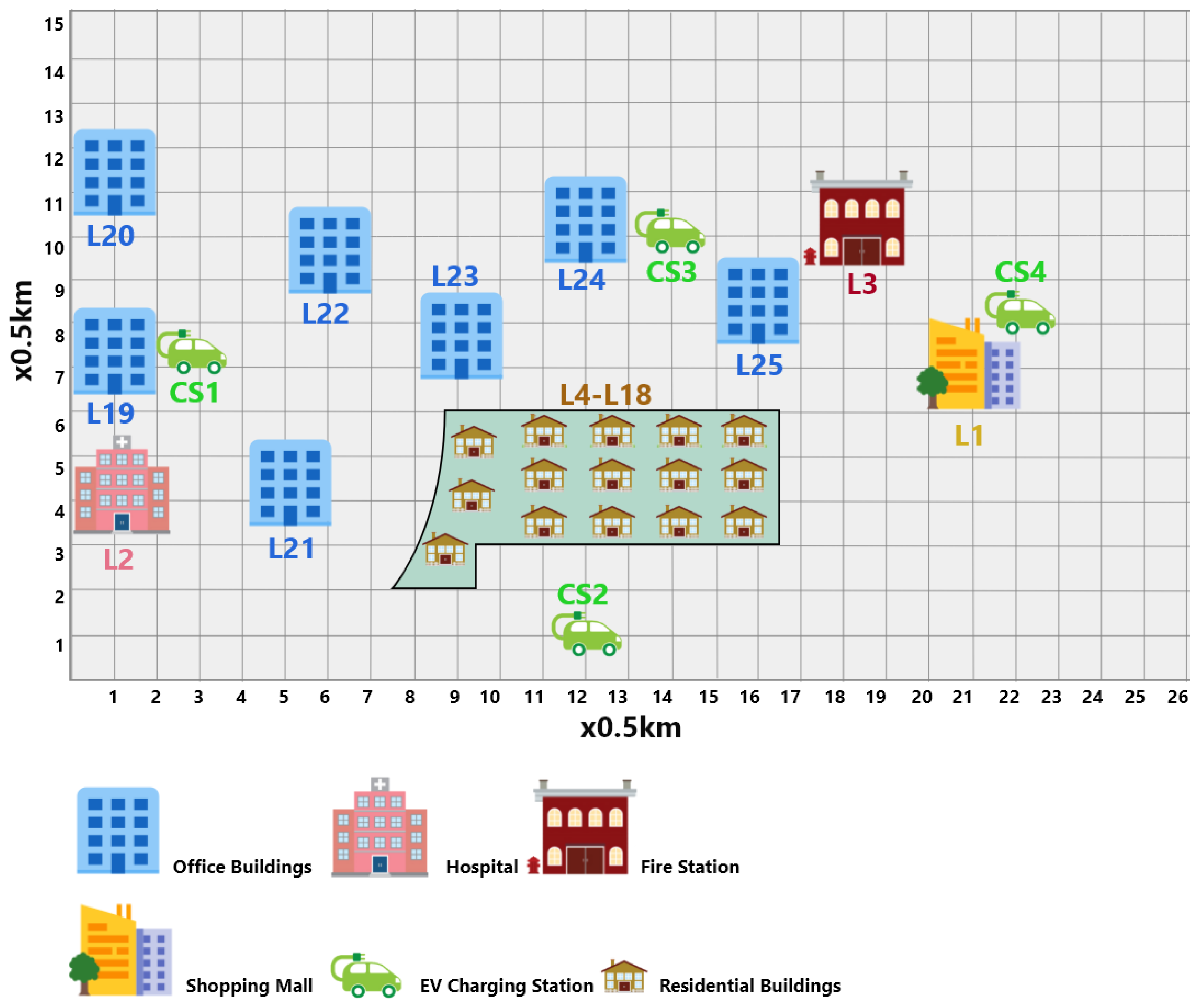
The schematic of the SC is presented in
Figure 4 and the coordinates of each building can be seen in
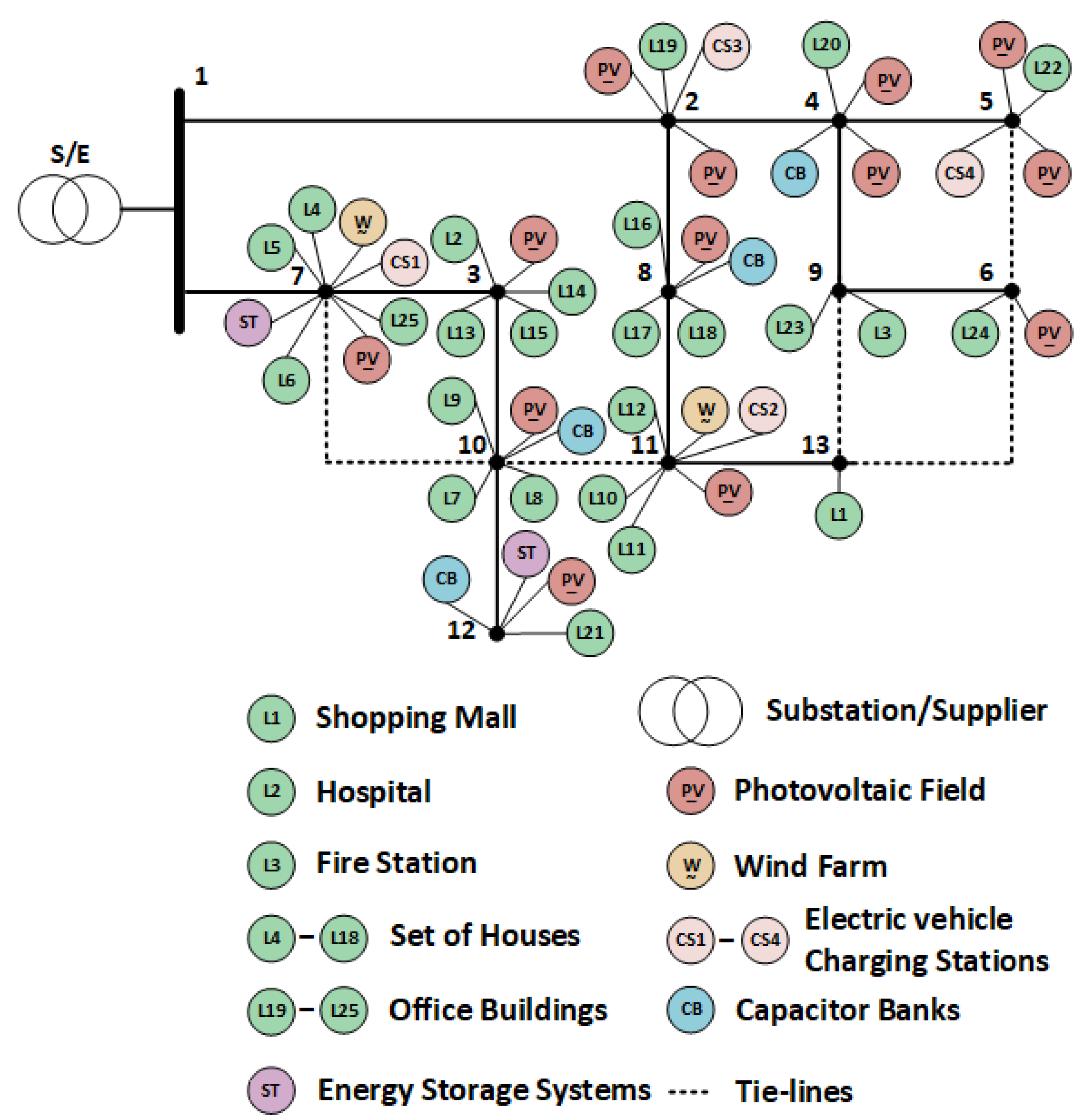
Table 3). The distribution network that feeds the entire city has one 30MVA substation and 25 load points. A total of 15 DG units (i.e., 2 wind farms and 13 PV parks), four capacitor banks of 1 Mvar, and are included in the network, as can be seen in
Figure 5. Moreover, the SC has seven parking lot buildings (commonly referred as charging stations in this research work) for EV charging, four (two in bus 7 and two in bus 11) slow charging lots (7.2 kW for each connection point) and three (two in bus 2 and one in bus 5) fast charging lots (50 kW for each connection point). Each slow charging parking lot has 250 spaces for EVs and 80 spaces for each fast charging parking lot building. The considered value for OPR is 30% leading to an ACNR value of 0.0132 €/kWh for a slow charging parking space and a value of 0.0919 €/kWh for a fast charging parking space. Additionally, the parking owner charges an additional 5% fee and 23% of value-added tax (VAT). Furthermore, it is considered that 50% of the EV users can charge their EVs at home (3.7 kW charge point) with a fixed cost of 0.2094 /kWh. The initial EV battery level is randomly generated between 40% and 65% of the battery capacity and the considered EV models, and their characteristics can be found in
Table 4.
Three user preference scenarios are considered, in one, the user’s priority is to charge their EV at a charging station located as close as possible to them. In the second scenario, the users prefer to find charging stations where they can charge their EV at a low price. In the third scenario, the EV user gives its preference to the charging time.
The line congestion cost is 0.02 €/kW when power flow is above 50% of the thermal line rating capacity.
The study presented in this research paper considers one week of input data for every 15 min with the aim of showing the effectiveness of the proposed model (i.e., 672 periods are considered in the simulation process). The chosen week is the 19 March 2017 to 25 March 2017.
This work has been developed on a computer with one Intel Xeon E5-2620 v2 processor and 16 GB of RAM running Windows 10 Pro. In addition to R language (for EV user behavior simulator), the MATLAB R2016a and TOMLAB 8.1 64 bits with CPLEX and SNOPT solvers were used for the optimization problems.
Simulations were performed using fixed and variable energy charging prices for two different populations scenarios, i.e., considering 2500 EVs and 5000 EVs. For each simulation, the following user preferences were changed: distance, price and charging time. The following features are fixed for all simulations in each population scenario:
The fixed charging prices are equal for all periods of the day and are 0.15 €/kWh for slow charge and 0.25 €/kWh for fast charge.
5. Results and Discussion
This section presents the results for the carried out simulations.
Section 5.1 presents the results for a scenario with 2500 EVs, while
Section 5.2 provides the results for a 5000 EVs population scenario.
5.1. Population Scenario with 2500 EVs
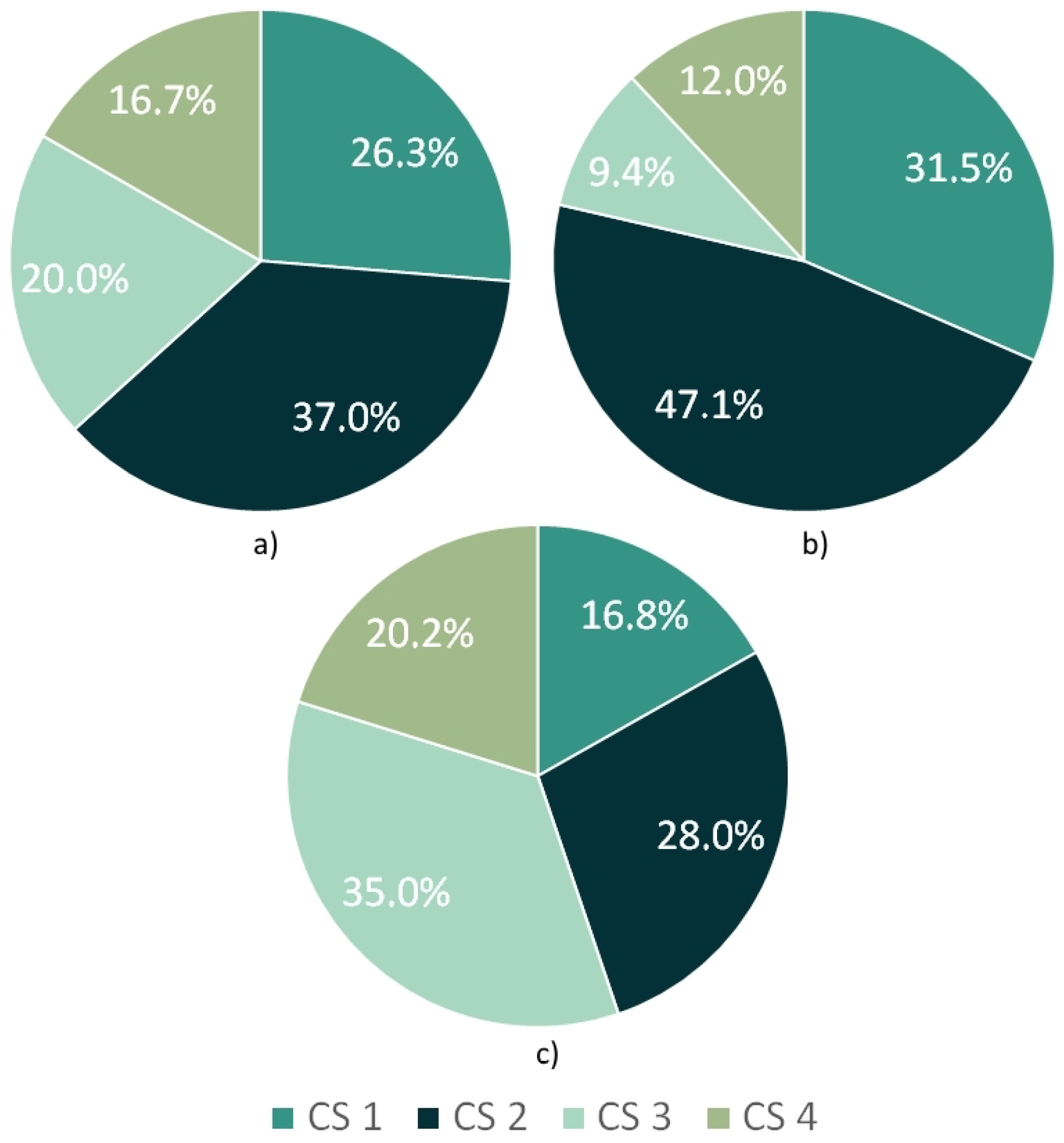
Considering a 2500 EVs scenario and using the fixed charging price, it is possible to see in
Figure 6 the correspondent charging sessions percentages for each user scenario preference (distance
Figure 6a, price
Figure 6b, and time
Figure 6c). It is worthy to note, that one charging session is counted from the moment the EV beings to charge until the time of it leaves the charging station. Analysing
Figure 6a (where the preference is the charging stations proximity to the total path that the user will have to do, i.e., the lowest sum value of the distance between the current location and the CS and the distance between the CS and the next EV user destination), it can be seen that the charging station 2 was preferred by users, with 37% of charging sessions. Since for this user preference scenario, the only differentiation between normal charging stations is the distance, and it can be concluded that CS 2 will be nearest to the users’ destinations when compared to the remaining CSs.
Figure 6b) (EV users’ gives priority to the price over the distance and charging time at the moment to chose a CS) shows that the CS 2 presents the higher charging sessions around 47% while the CS 1 was the second chosen one. The CS 3 and CS 4 (fast charging stations) presents together only a percentage around 21% of the total charging sessions. This is as expected result once the slow charging stations present lower charging prices compared to the fast charging stations. When the user time preference scenario is considered the majority of the users prefer the fast charging stations. As can be seen in
Figure 6c fast charging stations present 55.2% of the total charging sessions. However, this value also shows that the influence of the distance (CS 2 lower distance) and charging price (slow charging stations—lower price) have a strong influence on the users’.
Figure 7 depicts the charging sessions when the variable charging prices model is used. Like the fixed prices method when user distance preference is considered the variable model charging price also gives more sessions to CS 2 (
Figure 7a), leading to the same conclusion—this is the CS nearest to the users’ destinations. Checking
Figure 7b it is possible to conclude that CS 1 is the cheapest one due to the high percentage of charging sessions (71.7%). Regarding to the user time preference scenario (
Figure 7c), the results are very similar to the case where the fixed prices are considered, i.e., the majority of the users preferring the fast charging stations.
For the user distance and time preference scenarios, the fast charging station obtained a higher preference when compared to the case where the user preference is defined by the price. This indicates that when the price is not the most important factor, fast charging stations can attract users who are located close to them. Nevertheless, we concluded that the location of those charging stations is not optimal, because even when considering the user distance preference scenario, the majority of the users choose the slow charging stations—the cheapest ones. Moreover, to highlight this conclusion, when charging time is the most important factor the slow charging stations also present high preference, being the CS 2 the second most preferred.
A comparison between the fixed charging prices and the proposed variable charging prices model are shown in
Figure 8. As can be seen, the proposed model presents advantages in all scenarios for the EVs users in terms of charging prices. When the user distance preference scenario is considered, the proposed model presents 4% of gains for users’ (0.0083 €/kWh), for price and time user preference scenario the benefits are 10% (0.0210 €/kWh), and 2% (0.0046 €/kWh), respectively.
5.2. Population Scenario with 5000 EVs
In this subsection, it is presented the simulation results for a scenario with 5000 EVs.
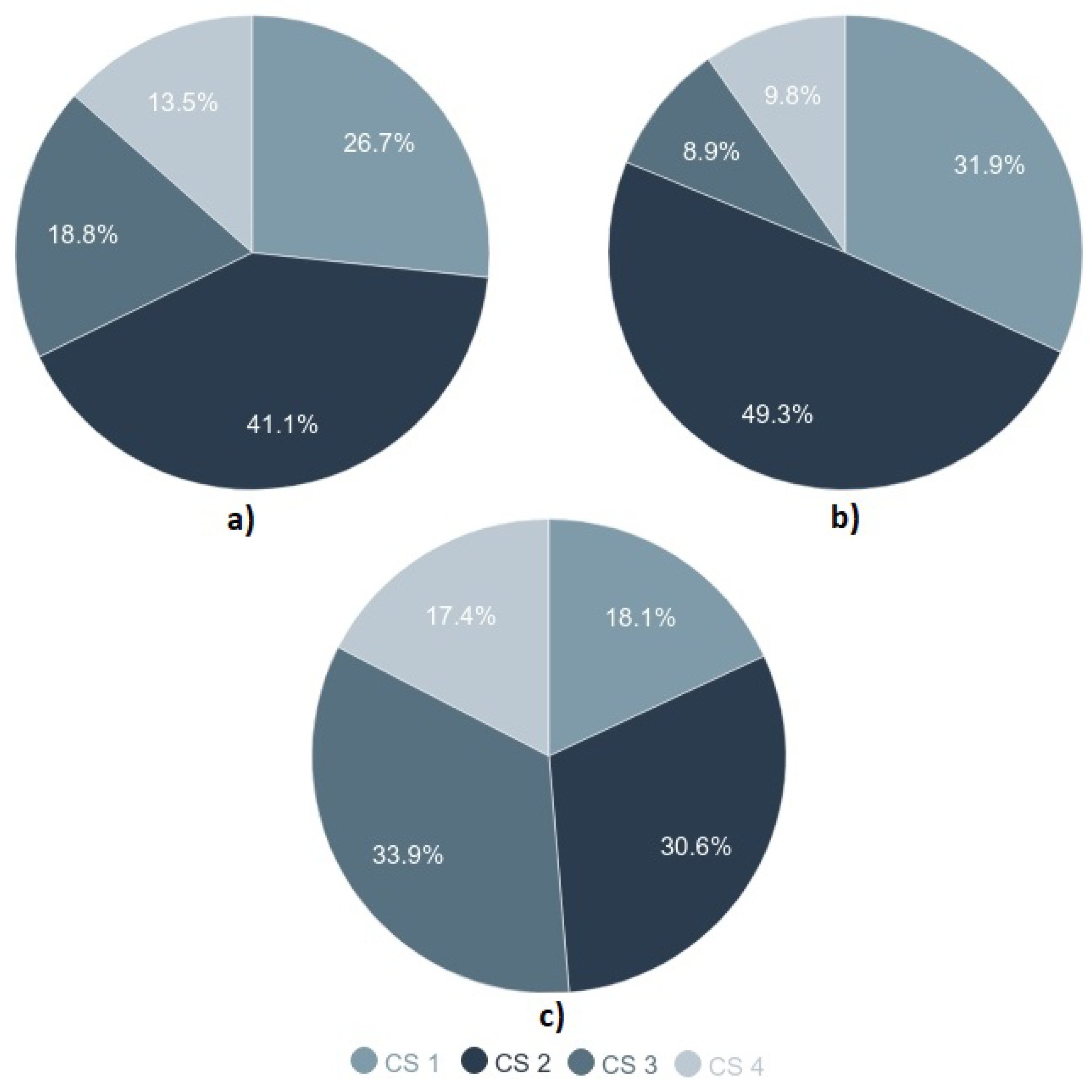
Figure 9 presents the charging session results for each Charging station in the three EV user scenarios preference considering fixed charging prices. The achieved conclusions are the same when the scenario with 2500 EVs is considered. Seeing
Figure 9a it is also checked through the presented values that CS 2 is near one to the users’ destinations. Also, when the price preference is considered, the slow charging stations are proffered (
Figure 9b), since they present the lower charging prices. When the charging time is crucial for the EVs users, the set of charging stations presents a percentage of charging sessions around 51% (
Figure 9c). Nevertheless, it is also verified that slow charging stations have a strong influence on the users’ choice.
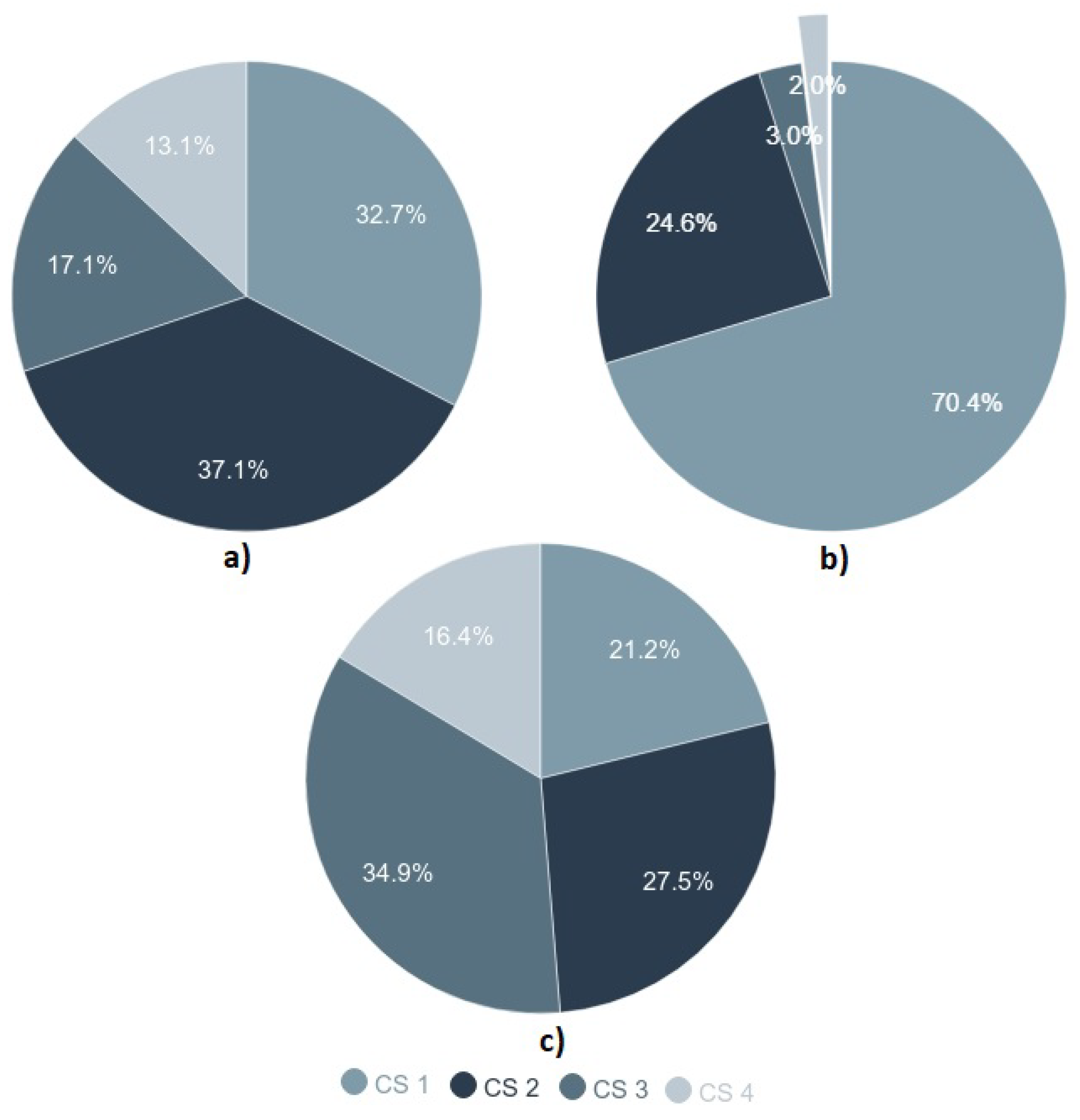
The charging sessions result considering the variable charging price model is depicted in
Figure 10. Once again, the results are very similar to the scenario with 2500 EVs, with more charging sessions in CS 2 when it is considered the user distance preference scenario (
Figure 10a)—CS 2 is the near one to the users’ destinations. For the user price preference scenario, the CS 1 presents the higher percentage of charging sessions (
Figure 10b). Thus, it can be concluded that CS presents more competitive charging prices compared to the remaining CSs. Considering the user time preference scenario, the higher percentage of EVs users’ (
Figure 10c) prefer the fast charging stations (51%).
The conclusions are the same when the scenario with 2500 EVs is considered, i.e., if time is not the most important factor, the users can be attracted by the fast charging station which can be closer to them. However, once again, it can be seen that the location of fast charging stations is not optimal (the majority of the users choose the slow charging stations even when the user distance preference scenario is considered). Also, as in the 2500 EVs scenario, when the most important factor for the users is the charging time, the slow charging stations also present a considerable preference, with the CS 2 as the second most preferred.
Figure 11 presents a comparison between the fixed charging prices and the proposed variable charging prices model. The proposed variable charging price model presents considerable advantages for the EVs users’ when distance and price preference scenarios are considered, with gains of 5% (0.0120 €) and 18% (0.0418 €), respectively. Regarding user charging time preference scenario the variable charging price model does not present advantages in terms of charge price for the EVs users when compared with fixed charging price (3% higher—0.0073 €).
6. Conclusions
This research paper presents a study of the impact of the variation of the energy charging prices on the behavior of electrical vehicle users. It also compared its benefits when using the variable and fixed charging prices. To this end, the authors developed an EV behavior simulator and combined it with an DLMP-based distribution network operation and reconfiguration optimization model. The main contributions of the conducted study can be summarized as follows: (1) EV user behavior simulator has been developed to generate a realistic population, considering the city size, and charging stations; (2) the positive impact of the variable EV charging prices on the electric vehicles users has been assessed.
The proposed methodology was tested in a case study which has been conducted on a mock-up model of a SC located at the BISITE laboratory with a 13 buses distribution network. Moreover, three users scenarios preferences (distance, price and time) were considered and were used to compare the results of the variable EV charging prices and EV fixed charging prices to demonstrate the advantage of the former.
It was verified that the use of variable pricing for EV charging is advantageous for the EV users in all scenarios when it is considered 2500 EVs. The gains are 4%, 10%, and 2%, respectively for distance, price, and time preferences. With 5000 EVs, the variable pricing does not present savings in comparison with the fixed charging prices when time scenario preference is considered. However, the proposed variable charging price model still presents considerable savings when the distance and price preference scenarios are considered. These two scenarios present for EV users 5% and 18% of gains, respectively.
The results suggest that the use of variable prices is promising, and can be used as an efficient approach in smart cities by offering to EVs’ users more options (in terms of price) when deciding where to charge their EVs.
The main disadvantages of the proposed model are: (a) the EV users profiles are not adapted to the different weekdays; (b) the decision charge method is only based on the battery charge level; (c) vehicle-to-grid is not considered.
In terms of future work, the authors will address more user profiles and additional charging decisions that depend on the energy price (increasing the flexibility), and also the possibility of vehicle-to-grid.
Author Contributions
The authors contributions were: Conceptualization, B.C., J.S., A.C., T.P., F.L., P.N., Z.V.; Methodology, B.C., J.S., A.C., T.P., F.L., P.N., Z.V.; Software, B.C., J.S., A.C., T.P., F.L., P.N., Z.V.; Validation, B.C., J.S., A.C., T.P., F.L., P.N., Z.V.; Formal analysis, B.C., J.S., A.C., T.P., F.L., P.N., Z.V.; Investigation, B.C., J.S., A.C., T.P., F.L., P.N., Z.V.; Writing—original draft preparation, B.C., J.S., A.C., T.P., F.L., P.N., Z.V.; Writing—review and editing, B.C., J.S., A.C., T.P., F.L., P.N., Z.V.; Visualization, B.C., J.S., A.C., T.P., F.L., P.N., Z.V.
Funding
This work has received funding from FEDER Funds through COMPETE program, from National Funds through FCT projects UID/EEA/00760/2019 and UID/CEC/00319/2019 and PTDC/EEI-EEE/28983/2017-CENERGETIC. Bruno Canizes is supported by FCT Funds through SFRH/BD/110678/2015 PhD scholarship. Angelo Costa is supported by the FCT Post-Doc Grant SFRH/BPD/102696/2014.
Conflicts of Interest
The authors declare no conflict of interest.
References
- United Nations. Chapter XXVII—Environment—7. d Paris Agreement. 2015. Available online: https://treaties.un.org/doc/Publication/MTDSG/Volume%20II/Chapter%20XXVII/XXVII-7-d.en.pdf (accessed on 17 April 2019).
- European Commission. Greenhouse Gas Emission Statistics—Emission Inventories; Technical Report; European Commission: Brussels, Belgium, 2018; Available online: https://ec.europa.eu/eurostat/statistics-explained/pdfscache/1180.pdf (accessed on 17 April 2019).
- Salah, F.; Ilg, J.P.; Flath, C.M.; Basse, H.; van Dinther, C. Impact of electric vehicles on distribution substations: A Swiss case study. Appl. Energy 2015, 137, 88–96. [Google Scholar] [CrossRef]
- European Environment Agency. Electric Vehicles and the Energy Sector—Impacts on Europe’s Future Emissions; Technical Report; European Union: Copenhagen, Denmark, 2017; Available online: https://www.eea.europa.eu/themes/transport/electric-vehicles/electric-vehicles-and-energy (accessed on 17 April 2019).
- Daina, N.; Sivakumar, A.; Polak, J.W. Electric vehicle charging choices: Modelling and implications for smart charging services. Transp. Res. Part C Emerg. Technol. 2017, 81, 36–56. [Google Scholar] [CrossRef]
- Latinopoulos, C.; Sivakumar, A.; Polak, J. Response of electric vehicle drivers to dynamic pricing of parking and charging services: Risky choice in early reservations. Transp. Res. Part C Emerg. Technol. 2017, 80, 175–189. [Google Scholar] [CrossRef]
- International Energy Agency. Global EV Outlook 2018; Technical Report; International Energy Agency: Paris, France, 2018; Available online: https://webstore.iea.org/global-ev-outlook-2018 (accessed on 17 April 2019).
- EVBox. Manifesto of Electric Mobility; Technical Report; EVBox: Amsterdam, The Netherlands, 2017; Available online: https://info.evbox.com/manifesto-electric-mobility (accessed on 17 April 2019).
- Corchero, C.; Gonzalez-Villafranca, S.; Sanmarti, M. European electric vehicle fleet: Driving and charging data analysis. In Proceedings of the 2014 IEEE International Electric Vehicle Conference (IEVC), Florence, Italy, 17–19 December 2014. [Google Scholar] [CrossRef]
- Franke, T.; Krems, J.F. Understanding charging behaviour of electric vehicle users. Transp. Res. Part F Traffic Psychol. Behav. 2013, 21, 75–89. [Google Scholar] [CrossRef]
- Marmaras, C.; Xydas, E.; Cipcigan, L. Simulation of electric vehicle driver behaviour in road transport and electric power networks. Transp. Res. Part C Emerg. Technol. 2017, 80, 239–256. [Google Scholar] [CrossRef]
- Neubauer, J.; Wood, E. The impact of range anxiety and home, workplace, and public charging infrastructure on simulated battery electric vehicle lifetime utility. J. Power Sources 2014, 257, 12–20. [Google Scholar] [CrossRef]
- Nicholas, M.A.; Tal, G.; Turrentine, T.S. Advanced Plug-in Electric Vehicle Travel and Charging Behavior Interim Report; Research Report—UCD-ITS-RR-16-10; Institute of Transportation Studies—University of California: Davis, CA, USA, 2017. [Google Scholar]
- Xu, M.; Meng, Q.; Liu, K.; Yamamoto, T. Joint charging mode and location choice model for battery electric vehicle users. Transp. Res. Part B Methodol. 2017, 103, 68–86. [Google Scholar] [CrossRef]
- Biegel, B.; Andersen, P.; Stoustrup, J.; Bendtsen, J. Congestion Management in a Smart Grid via Shadow Prices. IFAC Proc. Vol. 2012, 45, 518–523. [Google Scholar] [CrossRef]
- Bohn, R.E.; Caramanis, M.C.; Schweppe, F.C. Optimal Pricing in Electrical Networks over Space and Time. RAND J. Econ. 1984, 360–376. [Google Scholar] [CrossRef]
- Sotkiewicz, P.M.; Vignolo, J.M. Nodal pricing for distribution networks: Efficient pricing for efficiency enhancing DG. IEEE Trans. Power Syst. 2006, 21, 1013–1014. [Google Scholar] [CrossRef]
- O’Connell, N.; Wu, Q.; Østergaard, J.; Nielsen, A.H.; Cha, S.T.; Ding, Y. Day-ahead tariffs for the alleviation of distribution grid congestion from electric vehicles. Electr. Power Syst. Res. 2012, 92, 106–114. [Google Scholar] [CrossRef]
- Li, R.; Wu, Q.; Oren, S.S. Distribution Locational Marginal Pricing for Optimal Electric Vehicle Charging Management. IEEE Trans. Power Syst. 2014, 29, 203–211. [Google Scholar] [CrossRef]
- Liu, W.; Wu, Q.; Wen, F.; Ostergaard, J. Day-ahead congestion management in distribution systems through household demand response and distribution congestion prices. IEEE Trans. Smart Grid 2014, 5, 2739–2747. [Google Scholar] [CrossRef]
- Huang, S.; Wu, Q.; Oren, S.S.; Li, R.; Liu, Z. Distribution Locational Marginal Pricing Through Quadratic Programming for Congestion Management in Distribution Networks. IEEE Trans. Power Syst. 2015, 30, 2170–2178. [Google Scholar] [CrossRef]
- Krajzewicz, D.; Erdmann, J.; Behrisch, M.; Bieker-Walz, L. Recent Development and Applications of SUMO—Simulation of Urban MObility. Int. J. Adv. Syst. Meas. 2012, 5, 128–138. [Google Scholar]
- Axhausen, K.W. The Multi-Agent Transport Simulation MATSim; Ubiquity Press: London, UK, 2016. [Google Scholar] [CrossRef]
- Sewall, J.; Wilkie, D.; Merrell, P.; Lin, M.C. Continuum Traffic Simulation. Comput. Graph. Forum 2010, 29, 439–448. [Google Scholar] [CrossRef]
- de Arcaya, A.D.; Lázaro, G.A.; González-González, A.; Sanchez, V. Simulation Platform for Coordinated Charging of Electric Vehicles. In Proceedings of the 6th IC-EpsMsO: International Conference on “Experiments/Process/System Modelling/Simulation/Optimization”, Athens, Greece, 8–11 July 2015; pp. 8–11. [Google Scholar]
- Strehler, M.; Merting, S.; Schwan, C. Energy-efficient shortest routes for electric and hybrid vehicles. Transp. Res. Part B Methodol. 2017, 103, 111–135. [Google Scholar] [CrossRef]
- Mou, Y.; Xing, H.; Lin, Z.; Fu, M. Decentralized Optimal Demand-Side Management for PHEV Charging in a Smart Grid. IEEE Trans. Smart Grid 2015, 6, 726–736. [Google Scholar] [CrossRef]
- Bae, S.; Kwasinski, A. Spatial and Temporal Model of Electric Vehicle Charging Demand. IEEE Trans. Smart Grid 2012, 3, 394–403. [Google Scholar] [CrossRef]
- Soares, J.; Canizes, B.; Lobo, C.; Vale, Z.; Morais, H. Electric Vehicle Scenario Simulator Tool for Smart Grid Operators. Energies 2012, 5, 1881–1899. [Google Scholar] [CrossRef]
- Brooker, A.; Gonder, J.; Wang, L.; Wood, E.; Lopp, S.; Ramroth, L. FASTSim: A Model to Estimate Vehicle Efficiency, Cost, and Performance; SAE Technical Paper 2015-01-0973; SAE International: Warrendale, PA, USA, 2015. [Google Scholar] [CrossRef]
- V2G-Sim. Available online: http://v2gsim.lbl.gov/ (accessed on 17 April 2019).
- Alegre, S.; Míguez, J.V.; Carpio, J. Modelling of electric and parallel-hybrid electric vehicle using Matlab/Simulink environment and planning of charging stations through a geographic information system and genetic algorithms. Renew. Sustain. Energy Rev. 2017, 74, 1020–1027. [Google Scholar] [CrossRef]
- RStudio. Available online: https://www.rstudio.com/ (accessed on 17 April 2019).
- Canizes, B.; Soares, J.; Vale, Z.; Corchado, J.M. Optimal Distribution Grid Operation Using DLMP-Based Pricing for Electric Vehicle Charging Infrastructure in a Smart City. Energies 2019, 12, 686. [Google Scholar] [CrossRef]
- Conejo, A.J.; Carrión, M.; Morales, J.M. Decision Making Under Uncertainty in Electricity Markets; International Series in Operations Research & Management Science; Springer: Boston, MA, USA, 2010; Volume 153. [Google Scholar] [CrossRef]
- Soares, J.; Canizes, B.; Ghazvini, M.A.F.; Vale, Z.; Venayagamoorthy, G.K. Two-Stage Stochastic Model Using Benders’ Decomposition for Large-Scale Energy Resource Management in Smart Grids. IEEE Trans. Ind. Appl. 2017, 53, 5905–5914. [Google Scholar] [CrossRef]
© 2019 by the authors. Licensee MDPI, Basel, Switzerland. This article is an open access article distributed under the terms and conditions of the Creative Commons Attribution (CC BY) license (http://creativecommons.org/licenses/by/4.0/).

 ,
, 


