1. Introduction
Understanding the pressure state in the Austin Chalk and Eagle Ford shale reservoirs and their possible communication is important for petroleum engineering operations in several technical and proprietary ways. First, the pressure depletion history in each of the reservoirs controls the production rate of its wells. Since the Austin Chalk has been producing several decades prior to the development of the Eagle Ford Formation, knowing the state of their respective pressure depletion remains important for production forecasting and future field development planning.
Second, limiting pressure communication between adjacent reservoirs during hydraulic fracturing is important in order to minimize the loss of costly frack fluid and to avoid undue damage to pumps of nearby wells via unintended proppant pollution, a problem commonly faced by operators (reported by the managing director of E2 Operating, via personal communications with the authors on 29 October 2017). During a hydraulic fracture treatment proppant pollution is the invasion of proppants into the stimulated rock volume of an offset well. The fracture treatment can also affect the downhole equipment of offset wells.
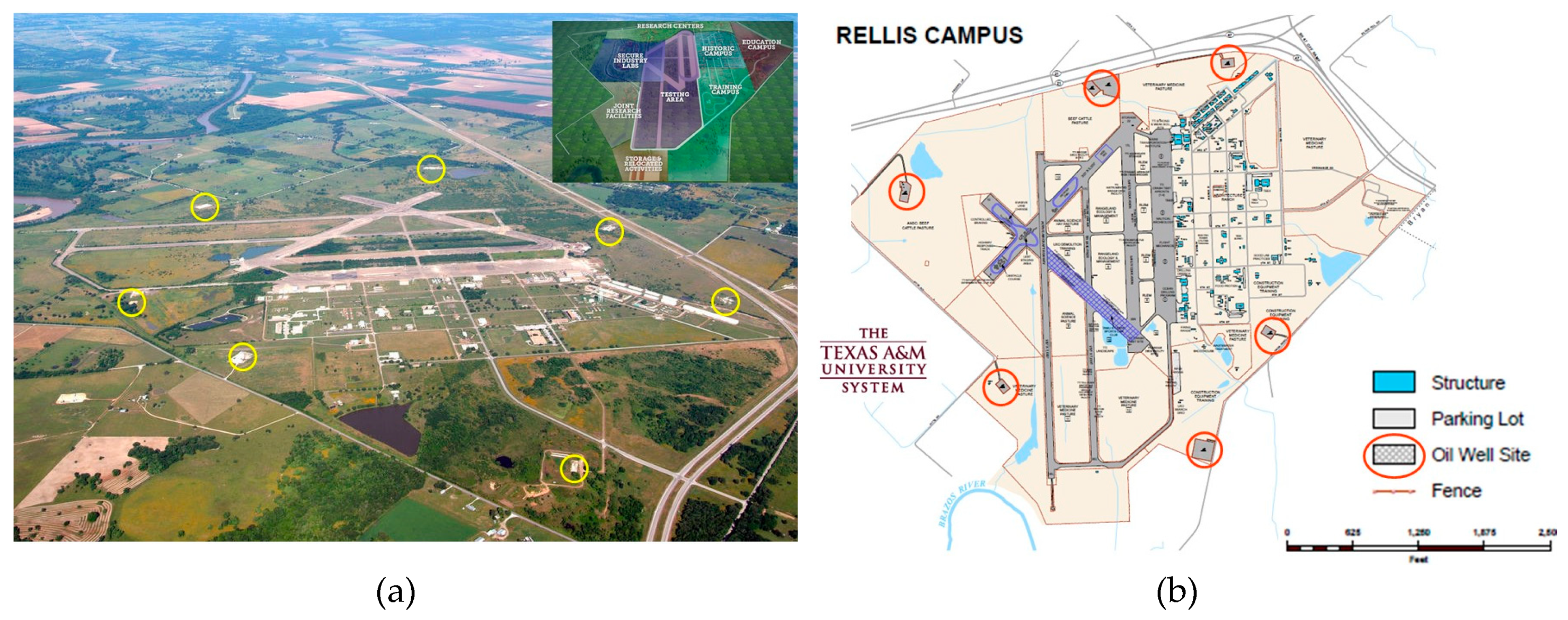
The main focus of this study is on the analysis of pressure response data of shut-in Austin Chalk wells during Diagnostic Fracture Injection Tests (DFIT) and subsequent zipper fracking of the two nearby Eagle Ford wells. Our study was conducted on a lease space beneath the RELLIS campus, a research facility that is administered by the Texas A&M University System in Brazos County (TX, USA). A physical image and schematic map of the RELLIS campus are displayed in
Figure 1a,b. The aerial view of the RELLIS Campus (
Figure 1a) highlights the relevant oil well site locations in relation to the schematic map (
Figure 1b). The images show that the individual wells considered are noticeably spaced apart. Interwell distances vary between several hundreds of ft to over a thousand ft (see later).
Our field study on the pressure communication between the wells of the individual companies was conducted using data provided by each of the operators (i.e., Austin Chalk and Eagle Ford leases, respectively). Well data are reported to the Texas A&M System in connection to their royalty share. Each reservoir is part of a split estate, which means that the mineral rights of the Austin Chalk and Eagle Ford Formation are leased to two different operators. Operators are pragmatic and have no incentive for judicial recourse in case of subsurface trespassing, which refers to the potential impact on mutual well productivity due to engineering interventions in adjacent petroleum reservoirs. Prior proceedings in the Texas High Court of Justice between adverse operators has declared the mutual responsibility to resolve any dispute lies with the individual operators [
1].
This study explains the reservoir setting and well layout, initial pressure state in both reservoirs (Eagle Ford and Austin Chalk), and then proceeds to report the pressure data collected. Our study confirms there exists no pressure communication between the two reservoirs, either prior to, or after the fracture treatment. However, a significant temporal pressure response was measured in the Austin Chalk legacy wells during both the 2017 DFIT and the zipper frac operations in the Eagle Ford landing zone. We analyze the initial pressure state, temporal changes induced during, and the final pressure state in each reservoir after the interventions. The second part of the paper presents a conceptual model that can explain the physical process of the interwell pressure communication based on the field pressure data analyzed in the first part of our study.
2. Project Overview and Data Acquisition
We have collaborated extensively with several operators in the Eagle Ford Formation below the RELLIS Campus and used the provided field data to develop pressure depletion models [
2,
3] and production forecasts [
4]. However, the overlying Austin Chalk Formation was developed in the early 1990s and although some logs are available from nearby wells in the formation, few details other than production data can be obtained for those older wells.
Six horizontal legacy wells, each with 4000 ft lateral length in the Austin Chalk reservoir landing zone beneath the RELLIS campus have either ceased to produce (3) or are marginal producers (3). These wells, named “Riverside 1 to 6” (or more simply R1 to R6) form the principal object of our study. The drilling and completion of two new wells in the Eagle Ford, with zipper fracking under extremely high hydraulic pressures used during fracture treatment of two Eagle Ford wells drilled in Nov/Dec 2017, provided a unique opportunity to gather pressure response data in the overlying Austin Chalk Formation via five pressure gauges, each mounted on a different Austin Chalk Riverside well.
2.1. Well Location and Trajectories
The Texas A&M University System administers the mineral rights of the RELLIS Campus in College Station, Texas, which includes the Eagle Ford shale, Austin Chalk and Buda Limestone plays that produce oil, and to a lesser degree, some associated natural gas. The development of the hydrocarbon plays (involving drilling, completion and necessary production operations such as shut-ins, artificial stimulations, including hydraulic fracturing and well workovers) is leased out to private operators. Our field study on the pressure communication between the wells of the individual companies was conducted using data provided by the various prior and current operators (i.e., for Austin Chalk and Eagle Ford leases, respectively). Well data are reported to the Texas A&M System in connection to their royalty share.
The RELLIS lease area hosts 12 wells drilled and completed during different epochs.
Table 1 displays the names and parameters of the wells studied, with the well specifics based on data from the Texas Railroad Commission. The six Austin Chalk legacy wells are currently owned by E2 Operating, a subsidiary of Exponent Energy, which acquired the wells in 2014 from a bankruptcy sale. There have been many changes in ownership of the Austin Chalk wells, which were first completed in 1990s, not further elaborated here, as can be traced via the Texas Railroad Commission. The more recently developed six Eagle Ford wells are currently operated by Hawkwood Energy (
Table 1), who bought the lease from Halcon Resources in 2017. Subsurface and production data were provided to us by various lease operators (i.e., E2 operation, Halcon Resources and Hawkwood Energy). All the companies mentioned in
Table 1 are oil and gas operators in Brazos county, Texas, USA.
A diagram of the well trajectories completed in the RELLIS lease area is shown in
Figure 2a. Eagle Ford Wells H2 and H3 were completed most recently (2017) and can be considered the child wells of parent Wells R, O, M, H1, all of which were completed in 2014.
Figure 2b illustrates the chronology of the development of the RELLIS lease area considered in our study. The dates of first production for the Eagle Ford Wells are the same as the dates of completion reported in
Table 1.
Prior to the recent rush to develop the Eagle Ford shale with modern multistage hydraulic fracturing techniques, only the Austin Chalk was developed in the RELLIS lease, because it is naturally fractured and production required only little well stimulation. Production for all the Austin Chalk wells started nearly three decades ago, first reported as of 1 July 1991, which is when the common production facility was completed for use by Well R1 initially. Each of the six Austin Chalk wells was fractured as a single stage with 7-inch casing and 30,000 bbl water, 11,000 lbs of diverter, and 18,000 gal of 15% hydrochloric acid. Additional completion data was not available. In 1992, the Austin Chalk Formation in Texas had a total of 4425 wells completed, which produced 330 million bbl of cumulative oil [
5]. A more recent well count gives the 9500 wells in total and a cumulative production of 1.7 billion BOE [
6]. The Austin Chalk, however still contains a large amount of unrecovered hydrocarbon resources, so the expansion of exploration in this formation could prove to be very profitable [
6].
2.2. Initial Pressures of the Austin Chalk and Eagle Ford Hydrocarbon Reservoirs
Three of the six Austin Chalk wells have been recently plugged and abandoned (R2 and R5 in January 2018; R6 in spring 2019) by the operator to make room for building operations. Over the course of their lifespan from July 1991 to January 2018 (28 years of production), the six Austin Chalk wells have cumulatively produced 1 million bbl of oil and 3.5 bcf of natural gas. Wells R2, R5 and R6 were already not producing for several years and remaining producers R1, R3 and R4 were shut-in during the fracture treatment of Wells H2 and H3. Currently, of the three remaining Austin Chalk wells, one is inactive (not pumping) and the two active ones only produce a marginal 2–3 bbl/day.
Knowing the pressure of the Austin Chalk reservoir space immediately prior to the fracturing operation on Nov/Dec 2017 is relevant in order to better understand how the hydraulic pressure of Eagle Ford well stimulation communicated with the ambient pressure in the Austin Chalk reservoir space. The pressure depletion in the Austin Chalk reservoir just before the fracturing of Wells H2 and H3 can be estimated based on historic production and decline curves using production data from Texas RRC online.
2.2.1. Initial Pressure in the Austin Chalk Formation
All six original Austin Chalk wells (R1–R6) were connected to a single production gathering system. The cumulative hydrocarbon output of the aggregated production system since first production started is graphed in
Figure 3a. The monthly decline of the hydrocarbon production over the 27-year well-life is separately plotted in
Figure 3b. Note that all the gas produced in this formation is dissolved gas. For most of its production history, there existed no free gas under reservoir conditions since the reservoir pressure was above its bubble point pressure such that there was only liquid in the formation. Further, low productivity of Austin Chalk can be attributed to reduced reservoir pressures and dissolved-gas-drive mechanisms [
7]. The Riverside wells were operated by pump jack for most of their production histories.
Using monthly production data, the reservoir pressure near the Austin Chalk wells at the time of the fracture treatment in Wells H2 and H3 was modeled based on the material balance technique outlined in [
8], reproduced in Equation (1). The detailed methodology and parameters used are explained in
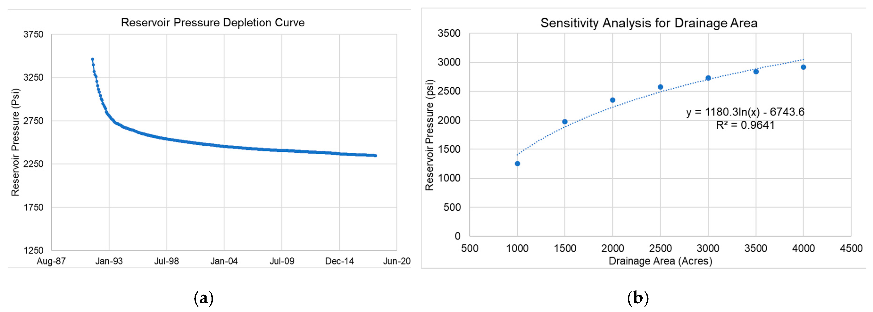
Appendix A. The pressure depletion curves obtained are shown in
Figure 4a. Keeping all other variables constant, a sensitivity analysis for the drainage area is presented in
Figure 4b, which shows that the effect of depletion is stronger for small drainage areas. The logarithmic correlation obtained indicates that the pressure depletion effect is dependent on the amount of hydrocarbon in place, which can be represented through drainage area, (with all other variables kept constant). The equation for original oil in place, (
) is presented in Equation (2). Details of the nomenclature/parameters used in Equations (1) and (2), assumptions made and method of the depletion calculation are further discussed in
Appendix A:
Based on
Figure 4a, the current reservoir pressure of the Austin Chalk is estimated at 2354 psi, corresponding to an assumed drainage area of 2000 acres, which is the approximate acreage of the RELLIS campus lease area [
9]. This value will be used in building a pressure response model (See
Section 4.4).
2.2.2. Initial Pressure Eagle Ford Formation
Although the Eagle Ford shale is an ultra-low permeability formation with negligible natural fractures in the area studied, the occurrence of pressure communication between Eagle Ford shale and the naturally fractured Austin Chalk would mean the fracture stimulation pump schedule may need adjustment when optimizing the fracking process.
The wells recently completed in the Eagle Ford Formation confirmed that the initial reservoir pressure remained intact [
2,
3], despite nearly three decades of oil and gas extraction in the overlying Austin Chalk Formation. The initial reservoir pressure of the Eagle Ford prior to first well completion in 2014 (
Table 1) was estimated based on history matching to be 4891 psi [
2].
The initial pressure in the Eagle Ford of 4891 psi is higher than the depleted state of the Austin Chalk, at 2354 psi. Interestingly, the lower pressure allows fluid to migrate to the Austin Chalk Formation during the fracking of wells in the Eagle Ford. We will further analyze the pressure communication between the Austin Chalk and Eagle Ford reservoirs during the 2017 fracture treatment.
2.3. Austin Chalk Pressure Gauges Monitoring Eagle Ford Zipper Fracking Operation
The main focus of this study is on the analysis of pressure response data of shut-in Austin Chalk wells during zipper fracking of the two nearby Eagle Ford wells. A gun barrel view of all the wells below the RELLIS lease area is shown in
Figure 5a to display well spacing and pressure gauge placements. Well spacing estimates are based on each well’s trajectory. The Eagle Ford wells were drilled such that all wellbore trajectories were mutually parallel and in the direction of minimum horizontal stress of the region, which is assumed to coincide with the direction of the regional dip towards the Gulf of Mexico. Eagle Ford well spacings could therefore be easily measured from a wellbore trajectory map. The Austin Chalk legacy wells spacings were estimated on a line of best fit perpendicular for each wellbore, extrapolating for R3 and R4. While reasonably accurate, the well spacings should therefore be taken as only estimates, as an uncertainty of ±100 ft exists.
Eagle Ford parent wells (R, O, M, H1) were drilled in 2014 (
Table 1). Eagle Ford child Wells H2 and H3 were drilled and completed in fall 2017, and were closely monitored for response in neighboring wells. In the case studied here, the operators adopted an optimized fracking approach called zipper fracking, which involved the staggered/alternating stimulation of the two wells on a stage by stage basis from toe to heel [
10], as shown in the timeline drawn in
Figure 5b. This is not to be confused with simultaneous fracking (“Simulfrac”), a similar technique in which the two wells are fractured simultaneously, saving valuable time for operators [
11]. In both cases, a primary aim (in addition to saving operation time and cost) is to create a network of complex hydraulic fractures, which can maximize stimulated rock volume, instead of fracturing linearly as with the traditional method [
10].
Figure 5b further shows that there is no overlap between the durations of any two stages, so each stage acts as a distinct source for pressure response. Although
Figure 5b shows only the timeline of the first 8 stages of Wells H2 and H3, we used and analyzed the pressure signals of all of the combined 101 stages involved in the fracturing operation (see
Section 2.4 and
Section 3.1).
2.4. Acquisition of Eagle Ford Pressure Data
The proprietary fracture treatment files for the Eagle Ford shale Wells H2 and H3 were supplied for our study by the operator. The files include stage by stage post stimulation reports, and data on all relevant fracture treatment parameters such as treating, wellhead, pump side, wellhead and surface casing pressures, slurry flowrates, proppant and mesh size, and additive concentrations, with respect to absolute time, at a frequency of one measurement per second for each quantity.
Table 2 shows the number of stages placed during the fracture treatment in each of the Eagle Ford well completions, along with the associated stage and cluster spacings. Wells H2 and H3, the subjects of our study, have the highest number of stages (51 and 50 stages respectively), and were fractured with an average of 9 clusters per stage.
Figure 5b showed the timeline for the 2017 fracture treatment progress for Wells H2 and H3. The base, start peak and end peak pressures are the three most important events for each stage of the fracture treatment and were therefore summarized and plotted (see
Section 3.1) to serve as a basis for correlation with the Austin Chalk response. In so doing, the voluminous data set supplied by the operator was significantly condensed, making it more suitable for further analysis. Eagle Ford well pumping schedules that were more prevalent in the recent past (2014), as well as common fracture treatment terminology used are discussed in
Appendix B.
2.5. Acquisition of Austin Chalk Pressure Data
The six Riverside wells were shut-in during the fracture treatment of Wells H2 and H3. Data logging pressure gauges were installed on the annuli of the Austin Chalk wellheads (Riverside 1–6) to measure any changes in the pressure. Processed data was logged at fifteen readings per minute. The time periods of successful and reliable data measurement for each well are reported in
Table 3. A chronology of the pressure data acquisition in the monitored wells is developed in
Figure 6. Diagnostic Fracture Injection Tests (DFIT) were conducted in both Wells H2 and H3 prior to the fracture operation in early November 2017, also shown in
Figure 6.
DFITs and other well testing procedures are more effectively investigated in more specialized work [
12]. In our study, we simplify the effect of this complicated procedure by considering the DFIT pressure rise in the toe of the two Eagle Ford wells (H2, H3) as a distinct source of potential pressure communication with the Austin Chalk wells.
The pressure response readings for Wells R1, R4 and R6 are continuous during the DFIT and subsequent fracture treatment of the Eagle Ford wells and are therefore considered more extensively in developing our models and formulating conclusions. Data from Well R2 is discontinuous and is limited to just two brief entries (Part 1 and Part 2) on
Figure 6. The pressure rise in Well R5 apparently killed the gauge early in the operation, so while the data set is continuous, it is not reliable data. The data collection period for Wells R2 and R5 ended permanently during the frack job. We attribute this to either memory overload or battery failure of the gauges. In spite of these technical issues, we were able to piece together a significant pressure response pattern by analysis of both the source and the response signals (
Section 3).
3. Analysis of Results
The well head pressure data for the Eagle Ford fracture treatment were condensed to obtain a simplified input pressure signal (
Section 3.1) that could then be used to visualize the correlation with the Austin Chalk pressure responses. The analysis of a fracture stage in the Eagle Ford is given in
Section 3.1.1 and the combined pressure signal is discussed in
Section 3.1.2. The correlated pressure response profiles are shown in
Section 3.2 for Wells Riverside 1, 4 and 6, while those of Riverside 2 and 5 are discussed separately in
Appendix C.
3.1. Pressure Analysis of Eagle Ford Wells H2 and H3
3.1.1. Analysis of Raw Data
Wellhead pressures for the fracture stages of the Eagle Ford wells provided by operators were used for later correlation with our pressure gauge measurements for Austin Chalk wells. The pressure build-up and subsequent pressure dissipation for Well H2 Stage 1 are shown in
Figure 7. Treatment graphs show wellhead pressure variations plotted along time for a given stage, along with other relevant quantities like slurry rate and proppant concentration on the same axes. The base, start peak and end peak pressures are the three most important events in each stage of the fracture treatment. The three primary pressure states during the fracture treatment of each individual stage are labeled on
Figure 7. Apart from minor operational differences, the treatment graphs for each stage in Wells H2 and H3 follow the same general pattern/shape of
Figure 7.
Start Peak Pressure: Highest pressure peak, which occurs at the very start of the plateau region of the pressure-time graph and corresponds to formation break down. Circulation fluid is pumped with no proppant to ensure the fractures are wide enough to accept the proppants, which is called creating a “pad”. Proppant circulation then typically commences at 100 mesh and low concentrations (20–50 ppg) and increases over time (terminology explained in
Table A2,
Appendix B). Sometimes during this process, a viscous proppant-free solution called “sweep” is used to remove any solid residuals and clean the well before circulating more proppant.
Base Pressure: Pressure that persists for a longer time, and is represented by the lowest pressure that occurred between the starting and ending peak pressures, which is the stable pressure required for injection of the constant rate of the slurry. Base pressure is attributed to fracture propagation in all directions away from the perforation, although preferential fracture growth occurs in the direction of maximum horizontal stress, perpendicular to the wellbore in the lateral direction [
13]. Wells H2 and H3 were fracked with 27 perforations per stage (on average). This being the first stage for Well H2 fracturing, acid was circulated after formation breakdown, after which proppants of increasing concentrations are circulated up to 100 mesh. In the region between the starting peak and base pressure, the fractures propagate in all directions, confined between assumed lower and upper frack barriers. Lateral growth is assumed for the period where the pressure is stable, and subsequently increasing with respect to time, that is, between the base pressure and ending peak. In a typical fracture treatment, operators seek to maximize lateral fracture propagation to maximize the stimulated rock volume, by orienting wellbores and initiating fractures accordingly.
End Peak Pressure: This corresponds to the time when pumping ceases and a pronounced end peak pressure occurs due to the highest proppant concentrations at the tip of the fracture (“screenout”). In order to avoid further pressure rise for Well H2 Stage 1 the operator cuts proppant supply. Operators need to be careful about pressure surges when ceasing pumping to end a stage. The goal is to regulate the proppant concentration precisely enough to minimize pressure build up towards the end of the stage. The final proppant concentration value for this well was 1.80 ppg at 100 mesh. Once this value was reached, the well was flushed with a fluid with no proppants to remove any residual acid and the stage was completed.
3.1.2. Pressure Summary for all Stages of Eagle Ford Fracture Treatment
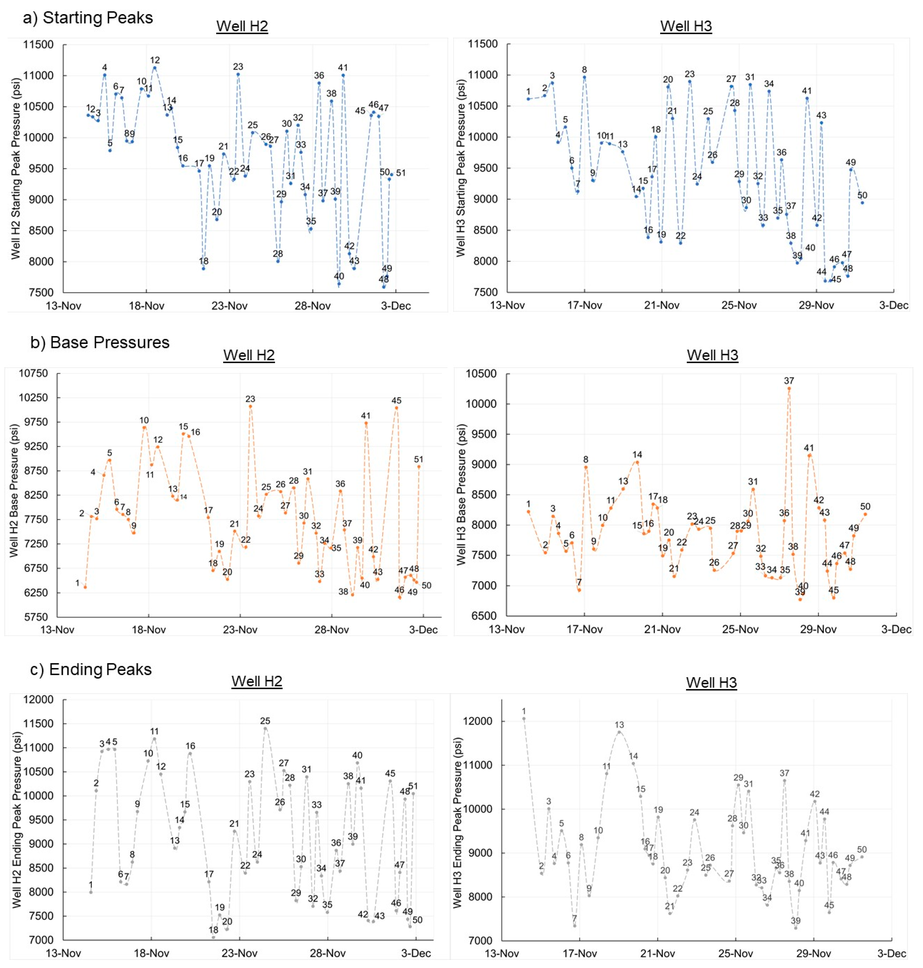
The post-stimulation reports provided by the operator were condensed by preparing summarized stage reports. The magnitudes of starting peak, base pressure and ending peak pressures of each stage in Wells H2 and H3 provide a first insight into the pressure profile, plotted in
Figure 8a–c respectively.
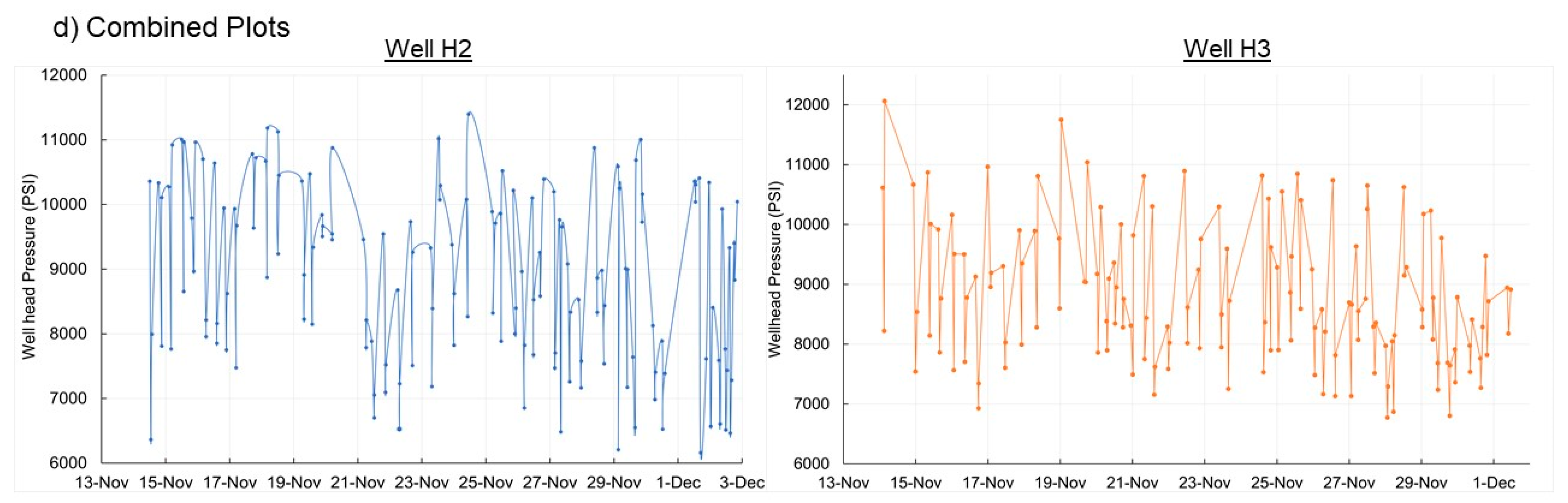
Figure 8d combines the starting peak, base peak and ending peak pressures in a combined plot for both wells. The plots provide an overview of the condensed Eagle Ford frack job pressure data against their relative timing. Next, the pressure signal of
Figure 8a–d will be used to explain the nature of the pressure communication with the Austin Chalk Formation.
3.2. Pressure Response of Austin Chalk (Wells R1–R6)
Pressure responses of the five monitored Austin Chalk wells (R1 through R6, except R3) are discussed in detail in our study. The Eagle Ford pressure signal in the plots produced in this section consists of the combined pressure sources for Wells H2 and H3 as individually condensed in
Figure 8d, but stage numbers are omitted in the correlated plots for the sake of clarity.
The following plots of Austin Chalk pressure response are based on high frequency pressure recordings (every 2 seconds) by the pressure gauges at the Austin Chalk wells. Given the difference in magnitudes between Eagle Ford and Austin Chalk pressures, the latter are plotted on a secondary axis (right-hand vertical scale in
Figure 9,
Figure 10 and
Figure 11), which produces one plot per well. Observations and interpretations made are displayed below each graph (
Table 3,
Table 4 and
Table 5). Pressure response profiles and interpretations of Wells R2 and R5 are discussed in
Appendix C.
3.2.1. Riverside 1
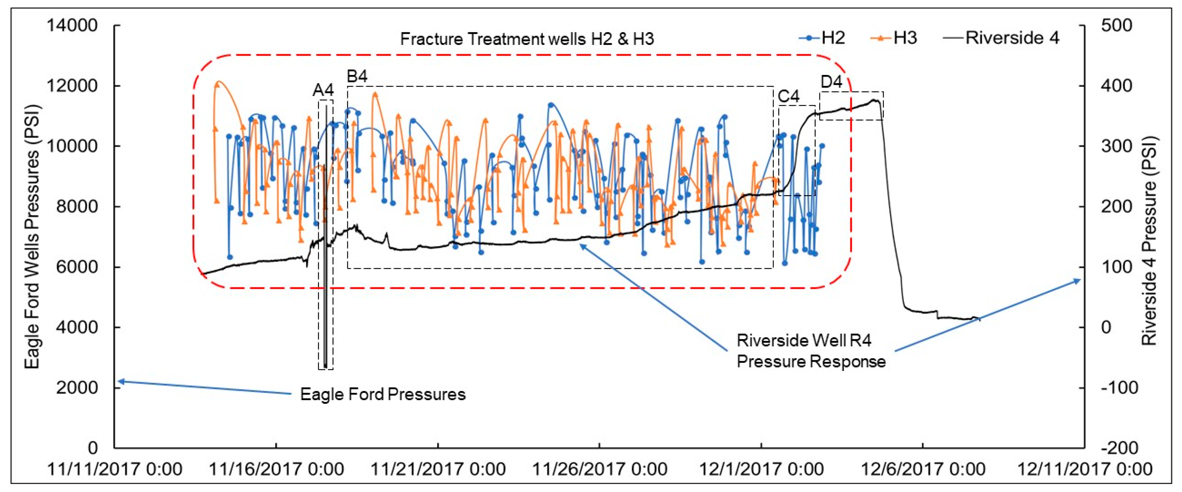
Figure 9 shows the correlations between the signal of the pressure sources of fracture treatment stages in Well H2 and H3, and the responses in Well R1 on an absolute time scale. The plot for Well R1 is annotated with more detail than for the other wells to establish the causes for pressure variations before and after the job. Little wriggles can be noticed in the flat trend of the R1 pressure response curve in region H1. These wriggles loosely correlate with the start of the stages, most likely due to formation breakdown or starting peak pressure. This trend holds for most of the Eagle Ford operation. Towards the end of the operation in region I1, there is a large increase in Well R1 pressure response that persists for a few days after the Eagle Ford frack job ceases for a certain time period, and then rapidly decreases. The steep drop of the pressure response curve is attributed to leakoff and final closure of the pressure conduit between Well R1 and the Eagle Ford pressure source, and can be observed to some degrees in all the wells.
Table 3 presents observations and interpretations for each region of the plot highlighted in
Figure 9. The table also specifies approximate date/time values for the selected regions. These observations will all be useful in developing a conceptual model for pressure communication in later sections, and recording time intervals will help in making further correlations.
3.2.2. Riverside 4
The correlated plot for Riverside 4 is shown in
Figure 10. The data for this well spans from just before the start of the fracturing in H2 and H3 and was collected until 12/8/2017, almost a week after the job in H2 and H3 ends. The plot highlights the important features of the pressure response profile (as in
Figure 9) whose durations are shown in
Table 4. Since the pre-frack data was not available, we cannot comment on the effect of the DFIT™ test conducted on 11/02/2017 on Riverside 4. Even so, the data set obtained for R4 is continuous, and is the most reliable out of all the wells studied (see
Figure 6) and shows strong response to the fracture treatment on the same time scale.
Table 6 also notes observations and durations associated with the regions of response highlighted in
Figure 10.
Similar to the response profile of Riverside 1 (
Figure 9), the little bumps on
Figure 10 correspond to the start of stages (most likely due to formation breakdown or starting peak pressure as we defined it) in region B4. Not all fracking stages produce visibly large bumps in the Austin Chalk. This trend holds for most of the Eagle Ford operation. Another similarity is in region C4 and region I1, where there is an increase in pressure towards the end of the operation. Region D4 marks the maximum pressure reached. However, unlike in Well R1 (region J1 labeled on
Figure 9) this maximum occurs over a plateau instead of one discrete point. We know that the maximum must be a plateau because the gradient of the plot decreases sharply between regions C4 and D4. Additionally, the pressure rapidly decreases in both Wells R1 and R4 after this maximum pressure point/plateau is reached. This is another important difference between R1 and R4, since in R4, the region of highest response occurs as a second plateau (with a noticeable, but minor positive gradient) instead of a discrete point, (as in Well R1), even though the maxima occur in both wells after the treatment is completed in Well H2. Further, the maxima in both Riverside wells occur at around the same absolute time (12/04/2017).
3.2.3. Riverside 6
The pressure response profile of Riverside 6 is shown on
Figure 11, and the observations and time durations were recorded in
Table 5. The key feature of this well is that there is only one significant pressure response in R6 that almost instantaneously occurs towards the end of the fracturing in Eagle Ford. Additionally, the magnitude of response is less than those of Riverside 1 and 4 (see
Figure 9 and
Figure 10 respectively) and takes significantly longer duration after the treatment ends to return to its initial reservoir state. Data for this well was collected until after the pressure returned to its initial state in about one week after the job ended. Similar to the highlighted region H1 (on
Figure 9) and B4 (on
Figure 10), the response for the majority of the frack job is characterized by a plateau region in pressure with wriggles loosely correlating with the starting times of stages. The selected region A6 (on
Figure 11) covers the entire frack operation. R6 follows the plateau trend of a steady pressure response for the almost the entire operation, unlike in Wells R1 and R4. Similar to R1 and R4, the pressure response of Well R6 peaks at the end of the operation and rapidly declines after reaching this maximum value. The difference in Well R6 is that the rise to this pressure occurs almost instantaneously, which could be attributed to equipment failure, but could also be a strong pressure communication between the wells. The significant pressure response commences almost instantly after the frack job in H2 is completed, unlike in R1 and R4 which began growing to a maximum after the job in H3 was complete, while the fracking of the final stages of Well H2 were still ongoing (recall the job for H2 was finished a day after H3 as shown in
Figure 8d). The pressure response maxima are reached at around the same time for Wells R1, R4 and R6 (i.e., at different times on 12/04/2017).
4. Interpretation of Results
The principal purpose of our study is to develop a conceptual model for the observed pressure communication between the two reservoirs (Eagle Ford and Austin Chalk). The estimated pressure acting on the boundary between the two reservoirs during the fracking of the Eagle Ford wells is modelled based on the pressure responses observed in the Austin Chalk wells discussed in
Section 3.2. Our analysis will quantify (and qualify) the correlation of the pressure response profiles using the following observations:
The relative lateral spacings between Eagle Ford Wells H2 and H3 and the Austin Chalk observation wells (
Section 4.1)
Changes in average production in wells in the vicinity of the H2–H3 pair, including impact on the Riverside production unit (
Section 4.2)
We then develop a conceptual model using the results of our analysis (
Section 4.3 and
Section 4.4) that serves to explain the principal mechanisms responsible for the observed pressure communication across the reservoir boundary between the Eagle Ford and the Austin Chalk Formations.
4.1. Vertical Communication
The reservoir pressures in the Eagle Ford an Austin Chalk reservoirs immediately prior to the the fracking operations in Wells H2 and H3 (
Section 2.2), and the Austin Chalk pressure responses during the fracture treatment (
Section 3.2 and
Appendix C) are used to better understand the detailed nature of the pressure communication between the Eagle Ford and Austin Chalk reservoirs. The principal pressure response magnitude, rate and durations for each of the observation wells are calculated in
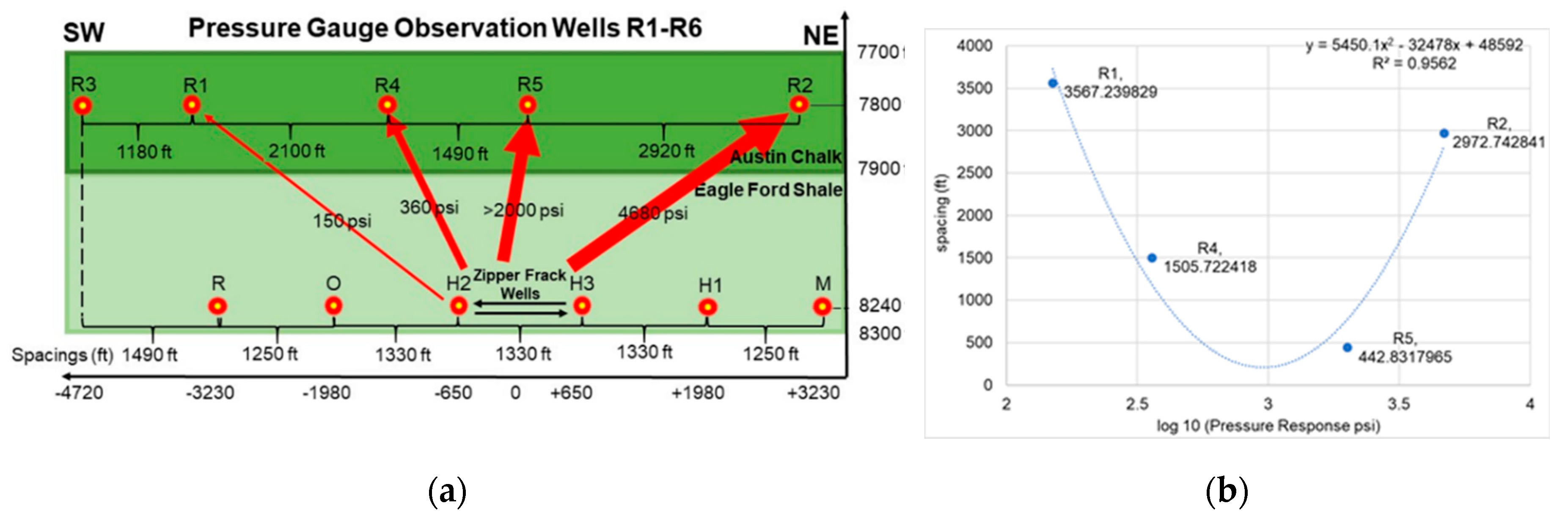
Appendix D. Pressure response magnitude is highlighted by the thickness of arrows in the gun barrel view of
Figure 12a, which shows that the pressure communication intensifies from SW to NE.
Based on the observations from
Figure 12a, one may suggest that the magnitude of pressure response is a function of distance to the fracked Wells H2 and H3. Diagonal spacings of Austin Chalk wells relative to the midpoint of H2–H3 pair are calculated and plotted against the logarithm of the pressure response in
Figure 12b, correlating the information presented in
Figure 12a. Diagonal well spacing and logarithm of pressure response therefore have a parabolic relationship. One possible explanation for the pressure communication intensifying from SW to NE is that a denser natural fracture network occurs in the NE part of the Austin Chalk, which establishes a better connection with the hydraulic fractures from the Eagle Ford. We assume that some hydraulic fractures in the vertical direction in the Eagle Ford wells will connect with a natural fracture, which will ultimately lead up to a Riverside wellbore. Natural fractures farther away from the wellbore have a better chance of activation if they fall within the influence zone of a long hydraulic fracture [
14]. Alternatively, some of the observed pressure communication may occur by fluid transmission through the primary pore network of the Austin Chalk, which has a 12% average porosity (in a potential range of 10% to 22%) and an average permeability of 0.12 mD (in a range of 0.01 md to 15 mD), according to local field studies [
7].
One may also speculate that the hydraulic fractures of Well H3 have wider apertures, because that well was fractured with coarser proppants (40/70 mesh heavy) much more frequently than Well H2 (100 mesh heavy), which would allow transmission of more frack-fluid and energy, and therefore could have resulted in a stronger series of connections with the natural fracture network in the Austin Chalk. In any case, Wells R2 and R5 show the highest intensity pressure response because these wells are relatively close to Well H3.
4.2. Observed Production Uplifts
Independent evidence for temporary pressure uplift in the Austin Chalk due to the fracking operation in the Eagle Ford Wells H2 and H3 is provided by increases in nearby Austin Chalk well productivity. For example, the Fazzino Well (API 04131486) operated by Wild Horse showed a distinct production uplift (
Figure 13), which more than doubled its production of both oil and natural gas on the time scale of the fracture operation, and persisted for several months afterwards. We reason that the natural fracture networks being activated through the intensity of the hydraulic fractures from the Eagle Ford is responsible for the uplift. The temporary pressure uplift observed resembles a fracture hit [
6,
15] which in our case did not result in permanent interwell communication. Earlier production uplifts seen in
Figure 13 can be attributed to well workovers and shut-ins. Typically, such periods of zero production are followed by brief episodes of enhanced production. However, no shut-in preceded the latest rise in the Fazzino well, which the operator therefore attributed to the nearby fracking operation in the Eagle Ford Wells H2 and H3.
Further, although Texas RRC reports that the Fazzino Well of approximately 3000 ft from the pressure signal (i.e., the H2–H3 Well pad), it is entirely possible that the production uplift observed was caused as a result of pressure communication due to the fracking of Wells H2 and H3. A similar incident occurred in 2014, in which a significant frack hit was observed in two other Eagle Ford wells in the same area. In that instance, Well O responded considerably to the fracking of Well H1, which is located 4000 ft away (in horizontal direction to the wells) from Well O.
Additionally, production data from the Texas Railroad Commission was considered in computing average changes in production for offset wells in the vicinity of the H2–H3 pair in the three months prior to and succeeding the fracture operation (which started on 14 November 2018). Three-month averages were computed for both oil and natural gas. The most significant production uplifts are summarized in
Table 6. Some of the production uplifts may have occured as a result of other refracks and workover operations taking place in the county at about the same time. Additionally, whether or not a well shows an average increase or decrease in production depends on how the average values are computed. For
Table 6, average before includes monthly data from August, September and October 2017 and average after includes December 2017, January and February 2018. However, the data in
Table 6 shows that the production uplift of the Fazzino Well emphasized in
Figure 13 is attributable to the fracture operations, given that
Table 6 reports 387% and 83% increases in oil and gas production, respectively.
4.3. Interpretations of Pressure Response Profiles and Conceptual Model
To build a conceptual model that can explain the temporary nature of and the physical process of pressure communication, we first consider the following additional details from the pressure response profiles presented in
Section 3.2. Our reference is the response of Riverside 1 (
Figure 9), but similar pressure response patterns and inferences were observed in the other Riverside wells (see
Figure 10,
Figure 11,
Figure A2 and
Figure A3)
The typical DFIT response [
16] is characterized by a sudden surge in pressure that is dominated by the input pressure signal, followed by a rapid release of pressure, known as the reservoir dominated region in which the reservoir returns to its original pressure state. Interestingly, the response patterns for the main fracture treatments of all five observation wells (see
Figure 9,
Figure 10 and
Figure 11,
Figure A2 and
Figure A3) also shows this pattern, to varying degrees. We identify four phases that characterize the pressure response pattern of Well R1, as follows:
- (1)
The first increase in pressure (regions F1 and G1 labeled on
Figure 9) is due to the hydraulic fractures propagating outwards in the vertical direction and connecting to the naturally fractured Austin Chalk system. As frack fluid enters the natural fracture network, the reservoir pressure of the Austin Chalk increases, which causes fluids to migrate towards Riverside wellbores, which were shut-in for the period of the fracking operation, but resumed production soon after the operation concluded. (Correspondingly,
Table 6 showed the later increase in both oil and gas production of the Riverside production pad, as a result of the fracture treatment, in the months following the operation).
- (2)
The plateau region (region H1 labeled on
Figure 9) can be attributed to the zipper fracturing nature of the operation. In a zipper fracking operation, the fractures propagate towards each other so that the induced stresses near the tips force fracture propagation in a direction perpendicular to the wellbores [
10]. The lateral fracture propagation prevents further vertical fracture growth, which results in a nearly constant pressure response in the Riverside well, given that each stage of the Eagle Ford fracture treatment was conducted in a similar way. The small bumps on the pressure response (region H1 labeled on
Figure 9) suggest that the Austin Chalk reservoir pressure would increase further, if not restricted by the induced stresses at the fracture tips caused by the zipper fracking operation. This method of zipper fracturing is also highly effective in creating an altered zone within the Eagle Ford itself (in the horizontal direction).
- (3)
The second increase in pressure (region I1 labeled on
Figure 9) begins towards the end of the treatment of Well H3. Since there is no more interference from an additional fracture treatment, the pressure increases until after the treatment of Well H2 ends, and pressure declines to its original state.
- (4)
The rapid decline in pressure occurs after a small time delay due to the residual effect of fracture treatment. If we model the entire response phenomena as a single fracture stage, the maximum response point (point J1 labeled on
Figure 9) would be analogous to a closure pressure after which the flow becomes reservoir dominated. Stress shadows are then able to close the induced/connected fractures and fracture fluid is no longer forced into the Austin Chalk. Correspondingly, the production uplift effect for the Riverside well pad declined over a longer time span, as was shown by production data for three months after the fracking operation ended (
Table 6).
The above pressure response observations for Well R1 largely apply to the other Riverside wells as follows:
Riverside 4: Although there is no early pressure increase in Well R4, the pressure is slowly increasing throughout the frack job (regions B4, C4 and D4 labeled on
Figure 10), and the magnitude of pressure communication is higher than for Riverside 1 (
Figure 9), suggesting that Riverside 4 has better communication with a naturally fractured zone, allowing for greater extent of fracture network development. The sudden spike in pressure in the middle of the fracture treatment job (Region A4 on
Figure 10) could mean that a direct fracture connection was formed, allowing for pressure to surge, that even momentarily stuns the gauge as shown by a momentary negative pressure value (region A4, labeled on
Figure 10). Similar to Riverside 1 (region I1 labeled on
Figure 9), Riverside 4 shows a second pressure increase (region C4 labeled on
Figure 10) at the end of the treatment of Well H3 that ends when the treatment of H2 ends, after which there is a slight increase for a short duration, due to the residual effect of the treatment. Reservoir dominated portion subsequently returns the reservoir to its original state.
Riverside 6: Similar to Wells Riverside 1 and 4 (region H1 labeled on
Figure 9, and region B4 labeled on
Figure 10 respectively), Well R6 shows a plateau region (region A6 labeled on
Figure 11) for the entirety of the frack job. The difference is that for Well R6, the increase in pressure (region B6 labeled on
Figure 11) occurs immediately after the end of the treatment of H2. The pressure subsequently declines in the same way as in Wells R1 and R4. The magnitude of communication is significantly lower in this well because it is spaced further apart from wells H2 and H3 than the other Riverside wells (Well R6 does not appear on the gun barrel cross section in
Figure 5a and
Figure 12a) Further, the lateral section of this well could have a weak connection to natural fractures, which means fewer hydraulic fractures can develop a network.
Riverside 2: Even though there is not enough data available, a region of pressure communication can be observed (Point B2 on
Figure A2), although it is followed by a sudden decline in pressure.
Riverside 5: Strong pressure surges are seen during and after the DFIT tests (conducted on Eagle Ford Wells H2 and H3 on 2 November 2017), in addition to observed response in middle of the fracture treatment (regions A5 and B5 respectively, labeled on
Figure A3). The surges once again can be attributed to events similar to those assumed for Riverside 1 (see above), except in this case in lieu of higher quality data, we conclude that the surges correspond to two discrete, strong connections being formed.
4.4. Conceptual Model
We assume that the Eagle Ford shale and Austin Chalk form a single hydrocarbon system, in which the Eagle Ford shale is the underlying source rock [
17].
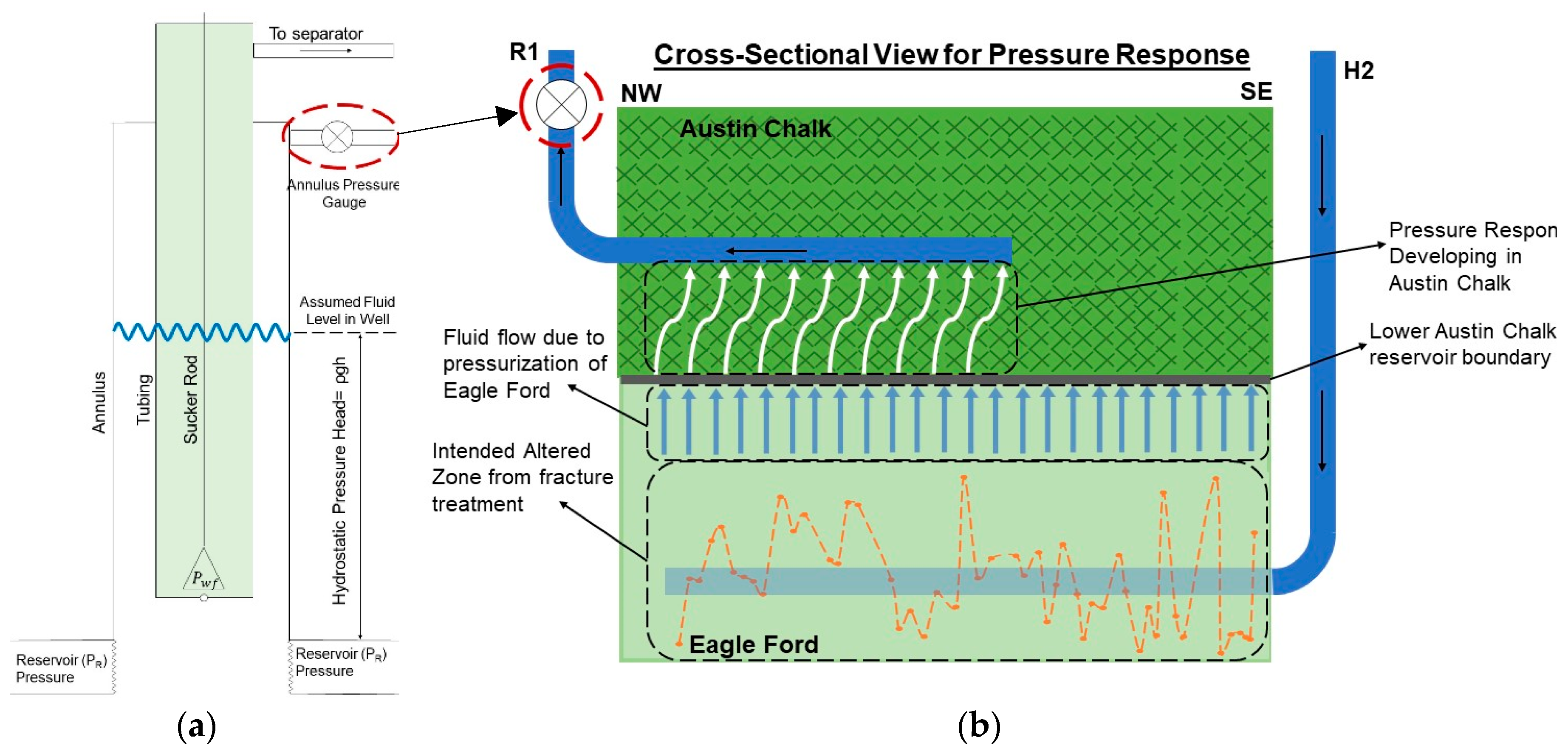
Section 2.2 showed that there exists a significant pressure (2354 psi) difference between the Eagle Ford and Austin Chalk Formations. The pressure difference could cause oil from the hydrocarbon-rich Eagle Ford shale to naturally migrate upwards into the lower pressured Austin Chalk Formation. However, without any form of human intervention, this migration must happen over geologic time, since both reservoirs have very low permeabilities. The hydraulic fracture treatment in the Eagle Ford pressurized the reservoir significantly and temporarily increased the pressure difference with the Austin Chalk. The hydraulic fracture treatment creates a fracture pattern in the Eagle Ford, which may connect to the existing natural fracture network in the Austin Chalk. Frack fluid used in the stage stimulation of Wells H2 and H3 is the ultimate source of the temporary pressure communication across the two fracture networks.
Figure 14a shows a schematic wellbore diagram of the vertical section of the Austin Chalk observation wells, highlighting the annular location of the wellhead where the pressure gauges were mounted.
Figure 14b shows a conceptual model for the observed pressure communication, with a vertical cross section of the reservoirs, taken perpendicular to the panel (of the gun barrel view) shown in
Figure 5a.
Figure 14b shows the base pressure signal introduced in
Figure 8b superimposed onto the lateral section to show the pressure experienced for the longest duration on each section of the wellbore over the course of the fracture treatment. Arrows indicate pressure transmission which ultimately causes pressure responses in Riverside wells. Pressure communication and fluid mobility in the model are both facilitated by the network of natural fractures in the Austin Chalk.
Often when fracture pressure communication is discussed, the observed pressure communication effects are attributed to changes in the in-situ stress of monitored well fractures, due to the propagation of hydraulic fractures in an offset well in the same reservoir, described further in [
18]. Poroelastic interactions between monitor fractures and propagating hydraulic fractures, for a general unconventional reservoir and well configuration, are also modeled in cases where the wells are in the same, typically shale, formation [
19]. These effects are not considered in our work since the Austin Chalk is a naturally fractured carbonate, which allows it to act as a conduit for actual physical fluid-based communication.
5. Conclusions
Our study analyzed empirical evidence for pressure communication with the Austin Chalk Formation during the stimulation of two new (2017 child) wells in the Eagle Ford shale, which caused the pressure to locally surge in both reservoirs. The conductive fracture network formed in the Austin Chalk is assumed to have transmitted some fluid pressure from the Eagle Ford to the annulus of five monitoring wells in the Austin Chalk. Pressure gauge responses in the Austin Chalk wells were measured during the fracture treatment in the Eagle Ford. The magnitude of pressure response in the Austin Chalk wells is only a fraction of the Eagle Ford injection pressures. The pressure stimulation of the two Eagle Ford wells occurred in alternating stages (zipper fracking).
The Riverside wells began responding to the Eagle Ford frack job through an initial increase in pressure as hydraulic fractures begin to propagate outwards and connect to the naturally fractured network of the Austin Chalk. The initial rise in pressure is followed by a plateau region, which is limited by the stresses induced in a zipper fracking operation that causes fractures to propagate towards each other, in a direction perpendicular to the wellbore. Immediately after the fracture treatment in Well H3 was completed, a second pressure rise occurred, which persisted until after the operation in Well H2 was completed. The pressure response rapidly declined to its pre-treatment state, which confirms that pressure communication was temporary in nature. The observed time delay was a result of stress shadows closing the induced/connected fractures, after which frack fluid is no longer forced into the Austin Chalk.
Our conceptual model of pressure communication takes into account the pressure depletion of the Austin Chalk reservoir due to decades of production, prior to the fracture treatment in the nearby Eagle Ford wells. The depleted, average reservoir pressure near the Austin Chalk wells is estimated to be 2354 psi. Based on history matching of earlier Eagle Ford (2014 parent) wells, the pressure in the Eagle Ford landing zone immediately prior to the fracture treatment was 4891 psi. The initial pressure in the annulus of the five Austin Chalk observation wells was approximately 20 psi immediately prior to the Eagle Ford fracture treatment. However, the pressure rose to 265.8 psi in Riverside 1, 378 psi in Riverside 4, and 63.3 psi in Riverside 6. Pressure response profiles of wells Riverside 2 and 5 show similar trends.
We summarize conclusions, based on our interpretations of the pressure response profiles in wells R1–R6, as follows:
- (1)
Pressure communication between the two well sets (Eagle Ford-Austin Chalk) is a temporary phenomenon, taking approximately up to three days (from the start of the zipper fracking of the H2–H3 Well pair) to establish, lasting approximately 11 to 12 days to reach a plateau, which is followed by a brief final screen out peak that drops off nearly instantaneously. In all the pressure response profiles considered, the pressure rise in the Austin Chalk wells rapidly declines back to pre-treatment annulus pressures.
- (2)
The magnitude of pressure rise in the Austin Chalk is significantly lower than Eagle Ford fracture treatment injection pressures (about 6%)
- (3)
Pressure communication is thought to occur due to pressurization of isolated fracture stages in the Eagle Ford wells, which temporarily increases the pressure differential between the Austin Chalk and Eagle Ford shale.
- (4)
Coeval production uplifts in the months following the fracking of the Eagle Ford wells were observed in the offset Austin Chalk wells, in addition to the Riverside wells themselves, and are associated with the natural fractured network of the Austin Chalk, that is further activated through the fracking of the Eagle Ford wells.
- (5)
Hydraulic fractures from the Eagle Ford open due to fluid injection during fracture treatment and are assumed to temporarily connect with the natural fracture system in the Austin Chalk reservoir. Poroelastic effects are not considered in our work due to the nature of the Austin Chalk.
- (6)
The pressure response in the annulus of the Austin Chalk wells is characterized by a time delay, because the pressure surges in Wells Riverside 1 and 4 ceased shortly after (35.2 h in Riverside 1 and 38.7 h in Riverside 4) the zipper fracking operation of Eagle Ford Wells H2 and H3 was completed.
Author Contributions
Data curation, S.S.; Investigation, S.S.; Methodology, R.W., I.A. and S.N.; Supervision, R.W.; Writing—review & editing, R.W. and S.S.
Funding
This project was sponsored by startup funds of the senior author (R.W.) from the Texas A&M Engineering Experiment Station (TEES).
Acknowledgments
We would like to thank Hawkwood Energy, Exponent Energy and the Texas A&M University System for providing access to the RELLIS lease wells and data sets, which facilitated our study. Tyler Moehlman is thanked for help as an undergraduate student collecting pressure data in the field.
Conflicts of Interest
The authors declare no conflict of interest.
Appendix A. Pressure Depletion Calculation in Austin Chalk
When the pressure in the Austin Chalk is below its bubble point pressure, the oil formation volume factor is given as a function of pressure as shown in Equation (A1). The formation volume factor
is an important parameter in calculating pressure depletion. Equation (A2) shows the calculation of pressure depletion from initial reservoir pressures based on production data. Equation (A2) is derived from material balance [
8]. The pressure in the reservoir can be iteratively calculated using monthly production data by solving Equation (A3) which is obtained from substituting Equation (A1) into Equation (A2) and solving for pressure
. Gas production is not a part of Equation (A2) (and hence Equation (A3)) since there is no free gas initially in the reservoir:
When the reservoir pressure is above the bubble point, the expression for formation volume factor changes, requiring the use of Equation (A4), which calculates the formation volume factor in an undersaturated reservoir. As in the below bubble point case, we substitute Equation (A2) to obtain the expression for pressure depletion, shown in Equation (A5), which needs to be solved using iterative techniques. The bisection method, which gives results to any desired level of precision (we use 0.01%) [
20] was used to solve Equation (A5):
The methodology adopted was to first calculate pressure depletion using Equation (A5) from monthly production data, replacing the initial reservoir pressure term
with the calculated pressure
after every interval. When pressure falls below the bubble point, Equation (A3) would need to be used instead. Using monthly production data (from Texas RRC online), we can calculate the resulting reservoir pressure at the time of the fracture treatment in Wells H2 and H3. All the parameters required for the above calculations (with nomenclature) are shown in
Table A1. The original reservoir pressure is first calculated from pressure gradient of 0.45 psi/ft and the average true vertical depth of the six Riverside wells. Petrophysical parameters are needed to perform original oil and water in place calculation. Although there is understandably a large uncertainty in values, we consider a scenario, in which the water saturation is the highest and therefore the percentage of water produced (to that of oil produced) is an arbitrarily chosen high value. The bubble point pressure and composition of the reservoir fluids present in the Eagle Ford are the same as that for the Austin Chalk vertically above, which is reasonable since the Austin Chalk and Eagle Ford shale likely form a single hydrocarbon production system [
17].
Table A1.
Variables used for pressure depletion model for Austin Chalk.
Table A1.
Variables used for pressure depletion model for Austin Chalk.
| Symbol | Parameter | Value | Unit |
|---|
| | Pressure Gradient | 0.45 | psi/ft |
| | True Vertical Depth (TVD) | 7731.3 | ft |
| Reservoir pressure before production | 3479.1 | psi |
| | Percentage of water produced | 50 | % |
| Rock Compressibility | | 1/psi |
| | Drainage Area | 4000 | acres |
| | Thickness | 200 | ft |
| | Water Saturation | 0.8 | No Unit |
| | Oil Saturation | 0.2 | No Unit |
| Initial Oil Formation Volume Factor | 1.15 | RB/STB |
| Initial Water Formation Volume Factor | 1.0 | RB/STB |
| | Porosity | 0.12 | No Unit |
| | Unit Conversion (for OOIP and OWIP calculation) | 7758 | Conversion |
| Original Oil in Place | | bbl |
| Original Water in Place | | bbl |
| Bubble Point Pressure | 2398 | psi |
| Undersaturated Oil compressibility | | 1/psi |
| Maximum Oil Formation Volume Factor | 1.16 | RB/STB |
The pressure depletion curves obtained are shown in
Figure 4a Keeping all other variables constant, we perform a sensitivity analysis for the drainage area and present the results in
Figure 4b, which shows that the effect of depletion is stronger for small drainage areas. For small drainage areas,
falls below the bubble point pressure, requiring use of Equation (A3) (see
Section 2.2.1 for
Figure 4a,b). The initial reservoir pressures plotted refer to the average of the reservoir pressures calculated for the duration of the fracture treatment. When the drainage area becomes infinitely large, the pressure depletion effect becomes negligibly small. Likewise, the reservoir pressure goes to zero for small drainage areas. The relationship is logarithmic in nature, with the correlations shown on the plot. Given that the RELLIS field spans over an area of 2000 acres [
9], we will use the corresponding reservoir pressure from
Figure 4a (2354 psi) in building our pressure response model.
Appendix B. Pumping Schedule of Well H1 in Fracture Treatment of 2014
This appendix presents pumping schedule used for hydraulic fracture treatment in Well H1, which is representative for all present wells (
Table 1) of the RELLIS area. Common terminology used in stimulation reports is also shown. The pumping process of 2014 fracture treatment of Well H1 was also similar to that used in 2017 fracture treatment of Wells H2 and H3. Wells were acidized, padded, and circulated with increasing levels of proppant concentration and decreasing proppant size as the stage progressed.
Figure A1 shows the treatment graph for Well H1 Stage 7 for comparison with pumping schedules of Wells H2 and H3, in
Figure 7. (shown in
Section 3.1). The most common terms used in a post-stimulation report are summarized in
Table A2.
Figure A1.
Well H1 Stage 7. The same properties apply as in Wells H2 and H3 (
Figure 7) except there is much more variation in Well H1, with regards to the proppants used, both in terms of grain and mesh size, which explains the high increase in proppant concentration (red line). In H2 and H3, 100 mesh is mostly used, with 40/70 being employed for select stages, so the corresponding graph would have a lower gradient or be flatter. Type of proppant and gels used are labeled.
Table A2.
Common fracturing terminology.
Table A2.
Common fracturing terminology.
| Term | Meaning |
|---|
| Start Peak Pressure | Wellhead pressure peak at the start of the job |
| Base Pressure | Minimum pressure that persisted for the longest time (in the plateau region) |
| End Peak Pressure | Wellhead pressure peak at the end of the job |
| Breakdown | The pressure/applied stress at which the formation breaks down |
| Acid | When acid is being circulated to loosen the formation |
| Shut Down | When pressure pumps shut down |
| Displace acid/Pump Ball | Stop circulating acid and start circulating slurry |
| Pad | Circulate fluid with no solid in it until the fracture is wide enough to accept proppant |
| Sweep | Circulate small volume of viscous fluid called a carrier gel to clean/remove solid residue from the well |
| Flush | Circulate a fluid that removes any remaining acid |
| End Stage | Indicates the end of stage. We may still take measurements for a few more minutes |
| x ppg 100 Mesh | When slurry at that proppant weight is circulated. Mesh is inversely proportional to grain size. 100 Mesh proppants are therefore fine-grained |
| x ppg 40/70 Mesh | When slurry at that proppant weight is circulated. 40/70 mesh proppants are coarser than 100 mesh. |
| ppg | A common unit of density; |
Appendix C. Pressure Response Profiles for Riverside 2 and Riverside 5
This appendix presents the pressure response profiles of Wells R2 and R5 in the same fashion as the profiles for Wells R1, R4 and R6 (shown in
Section 3.2) Not enough reliable data was collected for Wells R2 and R5 to produce a complete correlation, but results are still included since valuable insights can be gained from even the limited data available.
Riverside 2
The data collected for Riverside 2 is very limited (as discussed in
Section 2.5 and shown in
Figure 6). As a result, the pressure response profile shown in
Figure A2 consists mostly of interpolations (indicated by thin black lines). The data is sparse due to equipment failure, however
Figure A2 still shows that the gauges did detect an increased pressure in R2 during the treatment, even if for a short time. The data for Riverside 2 was unavailable after 11/27/2017, so B2 does not necessarily represent a maximum pressure. This would be since the gauge ran out of battery at that time or was otherwise unable to continue taking accurate readings.
Table A3 discusses the estimated point of increase and the approximate timings of events A2 and B2. The important observation from Well R2 response lies not in the correlation trend, but rather in the magnitude. Even for the minimal data connected, the figure shows the data in region B2 has magnitudes in regions of 3000 to 5000 psi, which is significantly more than Wells R1 and R4. Interestingly, there was no pressure response detected for the duration of the DFIT Test, even though pressure data was collected during this time (11/02/2017 to 11/03/2017).
Figure A2.
Correlated plots for Riverside 2. The left vertical axis is the pressure in Wells H2 and H3. The right axis is the pressure in the annulus of the Riverside wellhead. The significance of each labeled box is discussed in
Table 1. The lighter black lines in the plot are interpolations that connect between the missing data.
Table A3.
Observations and interpretations for Riverside 2.
Table A3.
Observations and interpretations for Riverside 2.
| Symbol | Comments/Interpretations |
|---|
| A2 | The point selected occurs on 11/15/2017 19:02 and corresponds to Wells H2 and H3 between stages 4 and 5. This point indicates the assumed start of pressure increase. For Well R2, the pressure increase approximates to a single straight line and takes place early on in the frac job. |
| B2 | 11/15/2017 13:15 H2 between stages 2 and 3, and H3 between stages 3 and 4. This point is the end of the pressure increase and what appears to be an instantaneous pressure drop. |
Riverside 5
The response profile for Riverside 5 presents almost no viable continuous data set, as shown in
Figure A3. While it is easy to assume this was caused by faulty gauges, the fact remains that there still does exist a pressure communication signal on the time scale of major events. Data is unavailable for Riverside 5 after 11/22/2017 05:21 AM. This well does not show any of the trends as the other Riverside wells studied. This would be since the gauge ran out of battery at that time or were otherwise unable to continue taking accurate readings.
Figure A3.
Correlated plots for Riverside 5. The left vertical axis is the pressure in Wells H2 and H3. The right axis is the pressure in the annulus of the Riverside wellhead. The significance of each labeled box is discussed in
Table A3.
Figure A3.
Correlated plots for Riverside 5. The left vertical axis is the pressure in Wells H2 and H3. The right axis is the pressure in the annulus of the Riverside wellhead. The significance of each labeled box is discussed in
Table A3.
Table A4.
Observations and interpretations for Riverside 5.
Table A4.
Observations and interpretations for Riverside 5.
| Symbol | Comments/Interpretations |
|---|
| A5 | The highlighted region is from 11/02/2017 10:13 AM to 11/04/2017 05:32 AM and corresponds to the DFIT™ test conducted on both wells on 11/02/2017 around 09:30 AM in Well H2 and 10:20 AM to 10:40 AM in Well H3. This should be the cause of the sudden rises and drops in the pressure. The pressure spike suggests that the pressure response was a surge strong and sudden enough to kill the gauge. |
| B5 | The region is from 11/21/2017 18:28 to 11/22/2017 05:21 AM, which corresponds to H2 between stages 19 and 20 and H3 between stages 22 and 23. The stimulation reports for these stages mention nothing unusual. The gauge picked up this spike even though it was potentially killed from the DFIT Test pressure response. |
The pressure gauges installed could read a maximum value of 2000 psi, which means the responses recorded for this well could exceed this value, since the highlighted regions indicate that the gauges were recording values beyond its maximum, which is what killed the gauge to begin with. As identified in
Table A4, Riverside 5 shows the strongest response to the DFIT test and fracture treatment of all the wells studied, which is identified even in the case of faulty equipment and an incomplete data set.
Appendix D. Austin Chalk Pressure Response Calculations
Table A5 describes in detail the pressure response calculations made for each Riverside observation well. Magnitude, duration and rate of pressure response in each of the Austin Chalk wells were determined from observations of the pressure response profiles of each well (shown in
Figure 9,
Figure 10 and
Figure 11,
Figure A2 and
Figure A3 respectively)
Table A5.
Rate, duration and intensity calculations for communications measured from available wellhead data. Timings are based on accurate date values.
Table A5.
Rate, duration and intensity calculations for communications measured from available wellhead data. Timings are based on accurate date values.
| Parameter | Value | Units | Comments |
|---|
| Riverside 1 |
| Average pressure | 21.42 | psi | Average wellhead pressure before DFIT™ test (until 10/31/2017 16:00, after that it increases sharply) |
| DFIT™ test intensity of response | 232.48 | psi | Peak value (C1 on Figure 9-Average. pressure |
| Duration of total response | 473.65 | hours | Duration of the total shape; start at 11/14/2017 14:15, 27 psi, end at 12/04/2017 07:54 |
| Rate of 1st increase | 1.073 | psi/hour | Average slope (pressure rise/duration); start at 11/14/2017 14:15, 27 psi, 11/20/2017 11:22, 178.4 psi |
| Duration of Plateau | 254.67 | hours | Duration of H1 block |
| Average response of plateau | 153.68 | psi | Average of plateau minus average pressure (175.1-21.43) =153.68 psi |
| Max response | 244.38 | psi | J1 Peak occurs on 12/04/2017 07:33 minus average |
| Rate of 2nd increase | 1.17 | psi/hour | Gradient of line from end of H1 block to J1 peak; use average response value of plateau to calculate; 77.52 hrs; |
| Duration of clustered region at the end | 41.92 | hours | Taken from 12/05/2017 23:55 to 12/07/2017 17:50 (end of data set) |
| Time delay to start response | Negligible | hours | Negligible time delay from the first stage data in Well H3 |
| Time delay after the job | 35.20 | hours | Between end of job in Well H2 and point J1 |
| Riverside 4 |
| Average pressure | 19.30 | psi | Taken from the end of the data set |
| Initial response | 81.80 | psi | This is the first pressure response including time delay on 11/16/2017 22:43; value-average |
| Time delay to start response | Negligible | hours | Time from the first Eagle Ford data point to initial response |
| Plateau region duration | 314.42 | hours | Consider region B4 |
| Plateau region avg response | 141.64 | psi | Plateau avg minus Avg. pressure 160.95-19.30 |
| Plateau region rate | 0.315 | psi/hour | 99.20/314.42 max-min/duration |
| Rate of 2nd increase | 5.19 | psi/hour | 121.1 psi/23.33 hrs; consider C4 |
| Max response | 358.70 | psi | Signifies end of response; Max-Average |
| Time delay end point | 38.67 | hours | Job end time to max point time |
| Rate of 2nd plateau | 0.6 | psi/hour | (378-352.9)/41.83; Consider region D4 |
| Riverside 6 |
| Average pressure | 14.18 | psi | Average pressure |
| Max response | 49.09 | psi | Max point minus average; 63.27-14.18; Other meaningful quantities cannot be calculated since the pressure rises almost instantaneously |
| Rate of decrease | 0.32 | psi/hour | This should be a negative value;(60.64-18.07)/131.67 |
| Riverside 2 |
| Average pressure | 148.48 | psi | Average pressure |
| Max response | 4676.82 | psi | Max point minus average; 4825.3-148.48 |
| Duration of response | 282.22 | hours | Time from A2 to B2; Time of interpolated line |
| Rate of response | 16.57 | psi/hour | Rate of increase for interpolated line; 4676.82/282.22 |
| Riverside 5 |
| Average pressure | 250.52 | psi | Taken from the flat region between the two responses |
| Duration of flat region between responses | 429.04 | hours | Taken from the flat region between the two responses |
| Duration of DFIT™ response | 43.32 | hours | First response; duration of A5 |
| Duration of start job response | 10.88 | hours | Second response; duration of B5 |
| Time delay for start job response | 184.25 | hours | Time when B5 region started minus time when the job started in H3 |
| Rate of response (gradient of flat region) | 0.409 | psi/hour | 175.3/429.04 |
References
- Rodgers, L. Subsurface Trespass by Hydraulic Fracturing: Escaping Coastal v. Garza’s Disparate Jurisprudence through Equitable Compromise. Tex. Tech Law Rev. Online Ed. 99. 2013, 45. Available online: http://texastechlawreview.org/volume-45/ (accessed on 2 November 2018).
- Khanal, A.; Weijermars, R. Pressure depletion and drained rock volume near hydraulically fractured parent and child wells. J. Pet. Sci. Eng. 2019, 172, 607–626. [Google Scholar] [CrossRef]
- Weijermars, R.; Alves, I.N. High-resolution visualization of flow velocities near frac-tips and flow interference of multi-fracked Eagle Ford wells, Brazos County, Texas. J. Pet. Sci. Eng. 2018, 165, 946–961. [Google Scholar] [CrossRef]
- Hu, Y.; Weijermars, R.; Zuo, L.; Yu, W. Benchmarking EUR estimates for hydraulically fractured wells with and without fracture hits using various DCA methods. J. Pet. Sci. Eng. 2018, 162, 617–632. [Google Scholar] [CrossRef]
- McGowen, H.E.; Krauhs, J. Development and Application of an Integrated Petroleum Engineering and Geologic Information System in the Giddings Austin Chalk Field. Soc. Pet. Eng. 1992. [Google Scholar] [CrossRef]
- Parshall, J. Can Austin Chalk Expansion Lead to Revival? Soc. Pet. Eng. 2017. [Google Scholar] [CrossRef]
- Hester, C.T.; Walker, J.W.; Sawyer, G.H. Oil Recovery by Imbibition Water Flooding in the Austin and Buda Formations. Soc. Pet. Eng. 1965. [Google Scholar] [CrossRef]
- Dake, L.P. Fundamentals of Reservoir Engineering, 8th ed.; Elsevier: Amsterdam, The Netherlands, 2001. [Google Scholar]
- Weijermars, R.; Burnett, D.; Claridge, D.; Noynaert, S.; Pate, M.; Westphal, D.; Yu, W.; Zuo, L. Redeveloping depleted hydrocarbon wells in an enhanced geothermal system (EGS) for a university Campus: Progress report of a real-asset-based feasibility study. Energy Strategy Rev. 2018, 21, 191–203. [Google Scholar] [CrossRef]
- Rafiee, M.; Soliman, M.Y.; Pirayesh, E. Hydraulic Fracturing Design and Optimization: A Modification to Zipper Frac. Soc. Pet. Eng. 2012. [Google Scholar] [CrossRef]
- Vermylen, J.; Zoback, M.D. Hydraulic Fracturing, Microseismic Magnitudes, and Stress Evolution in the Barnett shale, Texas, USA. Soc. Pet. Eng. 2011. [Google Scholar] [CrossRef]
- Craig, D.P.; Barree, R.D.; Warpinski, N.R.; Blasingame, T.A. Fracture Closure Stress: Reexamining Field and Laboratory Experiments of Fracture Closure Using Modern Interpretation Methodologies. Soc. Pet. Eng. 2017. [Google Scholar] [CrossRef]
- Economides, M.J.; Hill, A.D.; Ehlig-Economides, C.; Zhu, D. Petroleum Production Systems, 2nd ed.; Prentice Hall: Upper Saddle River, NJ, USA, 2013; Available online: http://ezproxy.library.tamu.edu/login?url=http://search.ebscohost.com/login.aspx?direct=true&db=cat03318a&AN=tamug.4023753&site=eds-live (accessed on 2 November 2018).
- Daneshy, A. Effect of Dynamic Active Fracture Interaction DAFI on Activation of Natural Fractures in Horizontal Wells. Soc. Pet. Eng. 2016. [Google Scholar] [CrossRef]
- Yu, W.; Wu, K.; Zuo, L.; Tan, X.; Weijermars, R. Physical Models for Inter-Well Interference in shale Reservoirs: Relative Impacts of Fracture Hits and Matrix Permeability. In Proceedings of the 4th Unconventional Resources Technology Conference, San Antonio, TX, USA, 1–3 August 2016. [Google Scholar] [CrossRef]
- Valko, P.P. Hydraulic Fracturing Short Course: Fracture Design, Fracture Dimensions, Fracture Modeling. 2005. Available online: http://slideplayer.com/slide/4948692/ (accessed on 10 November 2018).
- Martin, R.; Baihly, J.D.; Malpani, R.; Lindsay, G.J.; Atwood, W.K. Understanding Production from Eagle Ford-Austin Chalk System. Soc. Pet. Eng. 2011. [Google Scholar] [CrossRef]
- Seth, P.; Manchanda, R.; Kumar, A.; Sharma, M. Estimating Hydraulic Fracture Geometry by Analyzing the Pressure Interference Between Fractured Horizontal Wells. Spe Annu. Tech. Conf. Exhib. 2018. [Google Scholar] [CrossRef]
- Seth, P.; Manchanda, R.; Zheng, S.; Gala, D.; Sharma, M. Poroelastic Pressure Transient Analysis: A New Method for Interpretation of Pressure Communication Between Wells During Hydraulic Fracturing. Soc. Pet. Eng. 2019. [Google Scholar] [CrossRef]
- Chapra, S.C.; Canale, R.P. Numerical Methods for Engineers; McGraw-Hill: New York, NY, USA, 2015. [Google Scholar]
Figure 1.
(a) Aerial view of the RELLIS area (left image) highlights oil well sites (yellow circles); (b) Map view (right image) shows a more abstract schematic of the campus, with oil sites highlighted. Our study presents evidence of pressure communication between wells hundreds to thousands of feet apart.
Figure 2.
(
a) RELLIS wellbore trajectories. The white arrows represent the surface location of each well. The dotted outline represents the landing zone. The rectangular panel shows the portion of the gun barrel view introduced in
Section 2.3. Wells labeled R, O, M, H1, H2, H3 are completed in the Eagle Ford shale and wells labeled 1 to 6 are the Riverside wells completed in the Austin Chalk. The two Eagle Ford shale child wells, H2 and H3, are drilled from approximately the same location on the surface, and Wells H1, H2, H3 and O are mutually parallel. Wells H2 and H3 are 350 ft deeper at the toe (8450 ft) than at the heel side (8100 ft), due to a gentle slope of the producing landing zone of the wells. (
b) Chronology of development of RELLIS oil and gas lease area. Dates of well completion are displayed. The black bar represents a time lapse from 1996 to 2012. The Eagle Ford Wells (H1, H2, H3, R, O, M) are much younger than the Austin Chalk Wells (R1–R6) which have been operational for over 25 years.
![Energies 12 01469 g002]()
Figure 3.
(a) Cumulative production of the six Riverside wells (R1-R6). (b) Monthly production decline curves for six Riverside wells. Oil (blue curve) is measured in bbl and gas (orange curve) in Mcf.
Figure 3.
(a) Cumulative production of the six Riverside wells (R1-R6). (b) Monthly production decline curves for six Riverside wells. Oil (blue curve) is measured in bbl and gas (orange curve) in Mcf.
Figure 4.
(a) Pressure depletion curve for the Austin Chalk Formation with an assumed drainage area of 2000 acres. The depletion rate declines after long term production. (b) Sensitivity analysis for the effect of drainage area on reservoir pressure depletion. A strong logarithmic correlation is obtained.
Figure 5.
(
a) Pressure sources and positions. Gun barrel view of all the hydrocarbon wells completed in the RELLIS lease area used for our pressure communication study. Red arrows indicate possible connections between pressure signal source and the observation pressure gauges, which monitored the annulus pressures on wellheads of Wells R1-R6. No pressure gauge was mounted on Well R3. Section is taken from panel in
Figure 2a from South West to North East as outlined. Well R6 is outside the section and is therefore not shown in gun barrel. Well spacings are estimated using Well R3 as a reference line. The horizontal axis represents spacing relative to the midpoint of Wells H2 and H3. Vertical axis represents true vertical depth, and is exaggerated 6.6×. (
b) Pressure signal timeline. Example of timeline depicting the relative durations of the first 8 stages of the zipper frack operation for Wells H2 and H3 (around the clock). The inset table represents the order of events in the operation. There was a slight delay at the start of the project and Stage 1 in Well H2 began almost half a day later than in H3. The remainder of the procedure experienced no delays and the zipper frack pattern occurred with no incidents reported.
![Energies 12 01469 g005]()
Figure 6.
Chronology for Austin Chalk Pressure Data Collection. High quality pressure readings obtained from Wells R1, R4 and R6.
Figure 6.
Chronology for Austin Chalk Pressure Data Collection. High quality pressure readings obtained from Wells R1, R4 and R6.
Figure 7.
Fracture treatment graph for Stage 1 of Eagle Ford Well H2. All stages had a similar fracture treatment schedule.
Figure 7.
Fracture treatment graph for Stage 1 of Eagle Ford Well H2. All stages had a similar fracture treatment schedule.
Figure 8.
(a) Starting peak pressure (b) Base pressure, and (c) Ending peak pressure for each stage in Eagle Ford Wells H2 and H3, interpolated to more clearly show variation. Data points are labeled with corresponding stage number. Stage 1 is at the toe end and stage 51 and 50 are the final stages of the treatment, at the heel end of Wells H2 and H3, respectively. (d) Summary of Pressure change over time for 51 stage fracturing of Well H2 and 50 stage fracturing of H3. Data points represent discrete measurements and therefore the connections presented between data points are interpolations.
Figure 9.
Correlated plots for Riverside 1. The left vertical axis is the pressure in Wells H2 and H3. The right axis is the pressure in the annulus of the Riverside wellhead. The significance of each labeled box is discussed in
Table 3.
Figure 9.
Correlated plots for Riverside 1. The left vertical axis is the pressure in Wells H2 and H3. The right axis is the pressure in the annulus of the Riverside wellhead. The significance of each labeled box is discussed in
Table 3.
Figure 10.
Correlated plots for Riverside 4. The left vertical axis is the pressure in Wells H2 and H3. The right axis is the pressure in the annulus of the Riverside wellhead. The significance of each labeled box is discussed below.
Figure 10.
Correlated plots for Riverside 4. The left vertical axis is the pressure in Wells H2 and H3. The right axis is the pressure in the annulus of the Riverside wellhead. The significance of each labeled box is discussed below.
Figure 11.
Correlated plots for Riverside 6. The left vertical axis is the pressure in Wells H2 and H3. The right axis is the pressure in the annulus of the Riverside wellhead. Significance of each labeled box is discussed below.
Figure 11.
Correlated plots for Riverside 6. The left vertical axis is the pressure in Wells H2 and H3. The right axis is the pressure in the annulus of the Riverside wellhead. Significance of each labeled box is discussed below.
Figure 12.
(
a) Gun barrel view with pressure response intensity in monitored Austin Chalk wells emphasized by arrow width. Well spacings are estimated using Well R3 as a reference line. The horizontal axis represents spacing relative to the midpoint of Wells H2 and H3. Vertical axis represents true vertical depth, and is exaggerated 6.6× relative to the horizontal length scale. (
b) Plot of logarithm of pressure response against diagonal well spacings calculated from
Figure 12a. Data labels are the Austin Chalk well names (R1, R4, R5, R2) with measured diagonal spacings in ft. A strong parabolic correlation is obtained.
Figure 13.
Production profile of Fazzino Well, including a zoomed in section showing with greater resolution the production uplift attributed to the fracturing of Wells H2 and H3. The vertical axes for both plots have the same units. That is, bbl for oil and Mcf for gas. The production data used was obtained from the Texas Railroad Commission’s public sources.
Figure 14.
(a) Schematic wellbore diagram for the vertical section of an Austin Chalk observation well, showing static fluid column for a shut-in well and highlights (in red) the annular location on the wellhead where the pressure gauges were mounted. (b) Conceptual model illustrating fluid flow and pressure communication that ultimately cause production uplifts in the Riverside production unit.
Table 1.
Dates of completion of wells in the RELLIS lease area.
Table 1.
Dates of completion of wells in the RELLIS lease area.
| Symbol | Formation | Current Operator | Date of Completion | TVD (ft) | Lateral Length (ft) |
|---|
| R1 | Austin Chalk | E2 Operating LLC | 01 Jun 1991 | 7802 | 3258 |
| R21 | Austin Chalk | E2 Operating LLC | 01 Nov 1991 | 7628 | 4793 |
| R4 | Austin Chalk | E2 Operating LLC | 01 Dec 1991 | 7628 | 4233 |
| R3 (Not studied) | Austin Chalk | E2 Operating LLC | 01 Apr 1992 | 7844 | 3566 |
| R5 1 | Austin Chalk | E2 Operating LLC | 01 Nov 1992 | 7630 | 2508 |
| R6 1 | Austin Chalk | E2 Operating LLC | 01 Oct 1992 | 7856 | 3904 |
| R (Parent well) | Eagle Ford shale | Hawkwood Energy | 01 Apr 2014 | 8240 | 8630 |
| O (Parent well) | Eagle Ford shale | Hawkwood Energy | 01 Apr 2014 | 8240 | 2942 |
| M (Parent well) | Eagle Ford shale | Hawkwood Energy | 01 Nov 2014 | 8240 | 6550 |
| H1 (Parent well) | Eagle Ford shale | Hawkwood Energy | 01 Nov 2014 | 8240 | 5950 |
| H2 (Child well) | Eagle Ford shale | Hawkwood Energy | 31 Dec 2017 | 8240 | 7905 |
| H3 (Child well) | Eagle Ford shale | Hawkwood Energy | 31 Dec 2017 | 8240 | 7359 |
Table 2.
Number of stages, stage spacing and perforation cluster spacing used in fracking operations for six Eagle Ford Wells, Brazos County, Texas.
Table 2.
Number of stages, stage spacing and perforation cluster spacing used in fracking operations for six Eagle Ford Wells, Brazos County, Texas.
| Well Type | Well Name | No. of Stages (ft) | Stage Spacing (ft) | Perforation/Cluster Spacing (ft) |
|---|
| Parent | M | 20 | 300 | 50 |
| Parent | H1 | 22 | 300 | 50 |
| Parent | O | 13 | 240 | 60 |
| Parent | R | 35 | 250 | 63 |
| Child | H2 | 51 | 56–177 | 6–19 |
| Child | H3 | 50 | 45–180 | 6–20 |
Table 3.
Observations and interpretations for Riverside 1.
Table 3.
Observations and interpretations for Riverside 1.
| Symbol | Comments/Interpretations |
|---|
| A1 | Pressure variations due to well and offset wells production, which fluctuate due to rod-pump artificial lift. |
| B1 | Pressure begins to spike due to Diagnostic Fracture Injection Test (DFIT™) conducted on 11/02/2017, for both Wells H2 and H3 almost simultaneously. The highlighted region is the full period of the pressure spike in Eagle ford Wells during the DFIT test. |
| C1 | Pressure response spike was strongest on 11/03/2017 around 5:50 AM to 6:00 AM. Response increased up to 4000 psi for about one minute during this interval. Most likely an anomaly, but could also be an after effect of the DFIT™ test conducted the day before in which injection pressures increased up to 10,000 psi. About one minute of data is excluded from the response profile in Figure 9 due to outlier values (around 4000 psi) associated with the DFIT test. |
| D1 | More distinct pressure spikes could be from the operator restarting the pumping schedule after a pause |
| E1 | Same as A1 |
| F1 | This region is during 11/16/2017 and 11/17/2018, which corresponds to stages 7 to 9 on both Well H2 and H3. |
| G1 | Large increase in pressure during 11/17/2017 20:02 to 11/19/2017 19:50 corresponding to H2 stages 10,11 and 12 and H3 stages 10 and 11 (possibly also stage 12 but stage 12 data is unavailable) |
| H1 | The selected region is from 11/20/2017 11:22 AM to 12/01/2017 02:02 AM, which corresponds to H2 stages 17 to 43 and H3 stages 17 to 49. |
| I1 | The selected region is from 12/01/2017 00:00 to 12/04/2017 00:00. This corresponds to H2 stage 45 to 51 (end of job) to H3 stage 50 (last stage). Pressure response increases towards the end of the job in H3. |
| J1 | The peak pressure response of 265.8 psi occurs on 12/04/2017 07:33 AM and occurs after the operation is completed in both wells. Also, this is the maximum pressure reached mentioned in I1. |
| K1 | This surge occurs monetarily on 12/07/2017 01:47 AM after the operation is completed in both wells, and is attributed to anomalous data, potentially due to equipment failure |
| L1 | Anomalous data in this region (between 12/06/2017 to 12/07/2017) is attributed to equipment failure |
Table 4.
Observations and interpretations for Riverside 4.
Table 4.
Observations and interpretations for Riverside 4.
| Symbol | Comments/Interpretations |
|---|
| A4 | Pressure spike occurs on 11/17/2017 between 13:07 and 13:25. The surge momentarily stuns the gauge. The highlighted region corresponds to the interval between stages 9 and 10 on both Wells H2 and H3. |
| B4 | The selected region is from 11/18/2017 on 12:04 to 12/01/2017 14:29, corresponding to H2 stages 12 to 45 and H3 stages 13 to 50 (end of the job in H3). It also includes H3 stage 12, but the data for this stage is unavailable so it remains uncertain. |
| C4 | The region starts from 12/01/2017 17:51 to 12/02/2017 17:11, which corresponds to H2 stages 46 to 50. Pressure response increases almost immediately after the end of the job in H3. |
| D4 | The region starts from 12/02/2017 17:11 (same time as when region C4 ends) and ends at 12/04/2017 11:01, which corresponds to H2 stage 51 (last stage) but is after the job in Well H3. |
Table 5.
Observations and interpretations for Riverside 6.
Table 5.
Observations and interpretations for Riverside 6.
| Symbol | Comments/Interpretations |
|---|
| A6 | The plateau region starts from H2 stage 1 (11/14/2017 12:04) to H2 stage 51 (12/02/2017 20:21) and encompasses the entirety of the fracture treatment. |
| B6 | Similar to R1 and R4, the pressure peaks at the end of the operation, and rapidly declines after reaching this maximum value. The highlighted region is from 12/02/2017 20:21 to 12/03/2017 02:17AM. |
Table 6.
Offset production data. Changes in production are based on 3-month averages before and after November 2017.
Table 6.
Offset production data. Changes in production are based on 3-month averages before and after November 2017.
| Oil Production (bbl) |
| Name | API Number | Direction Relative to H2/H3 | Aug-17 | Sep-17 | Oct-17 | Avg before | Nov (during) | Dec-17 | Jan-18 | Feb-18 | Avg after | % Change |
| Riverside Production Unit | 04131502 | Direct South | 191 | 688 | 79 | 319 | 236 | 754 | 783 | 128 | 555 | 73.80 |
| Fazzino Omni | 04131486 | South West | 162 | 156 | 183 | 167 | 510 | 915 | 826 | 699 | 813 | 387 |
| Brazos Farm | 04131474 | North West | 6 | 0 | 0 | 2 | 284 | 449 | 259 | 205 | 304 | 15117 |
| Fazzino-Penicka | 04131530 | West | 137 | 124 | 150 | 137 | 169 | 189 | 173 | 153 | 171 | 25.3 |
| Willie Kuder | 04131464 | South West | 178 | 0 | 98 | 92 | 1 | 253 | 284 | 254 | 264 | 186.6 |
| Magnolia Oil & Gas | 04131307 | North West | 151 | 173 | 185 | 170 | 155 | 125 | 120 | 163 | 136 | −19.8 |
| Brazos Farm Ltd. | 04131462 | South West | 0 | 0 | 12 | 4 | 14 | 14 | 18 | 49 | 27 | 575 |
| Gas Production (Mcf) |
| Name | API Number | Direction Relative to H2/H3 | Aug-17 | Sep-17 | Oct-17 | Avg before | Nov (during) | Dec-17 | Jan-18 | Feb-18 | Avg after | % Change |
| Riverside Production Unit | 04131502 | Direct South | 969 | 2185 | 1682 | 1427 | 871 | 1768 | 1539 | 1157 | 1488 | 4.29 |
| Fazzino Omni | 04131486 | South West | 368 | 460 | 684 | 602 | 897 | 1105 | 1234 | 967 | 1102 | 82.98 |
| Brazos Farm | 04131474 | North West | 32 | 0 | 0 | 153 | 580 | 735 | 606 | 372 | 571 | 273.20 |
| Fazzino-Penicka | 04131530 | West | 1217 | 1127 | 1180 | 1163 | 1129 | 1193 | 1137 | 999 | 1110 | −4.61 |
| Willie Kuder | 04131464 | South West | 1811 | 1993 | 1143 | 1560 | 1296 | 995 | 478 | 692 | 722 | −53.76 |
| Magnolia Oil & Gas | 04131307 | North West | 254 | 223 | 274 | 250 | 279 | 240 | 260 | 262 | 254 | 1.46 |
| Brazos Farm Ltd. | 04131462 | South West | 19 | 15 | 12 | 15.3 | 12 | 0 | 0 | 0 | 0 | −100 |
© 2019 by the authors. Licensee MDPI, Basel, Switzerland. This article is an open access article distributed under the terms and conditions of the Creative Commons Attribution (CC BY) license (http://creativecommons.org/licenses/by/4.0/).


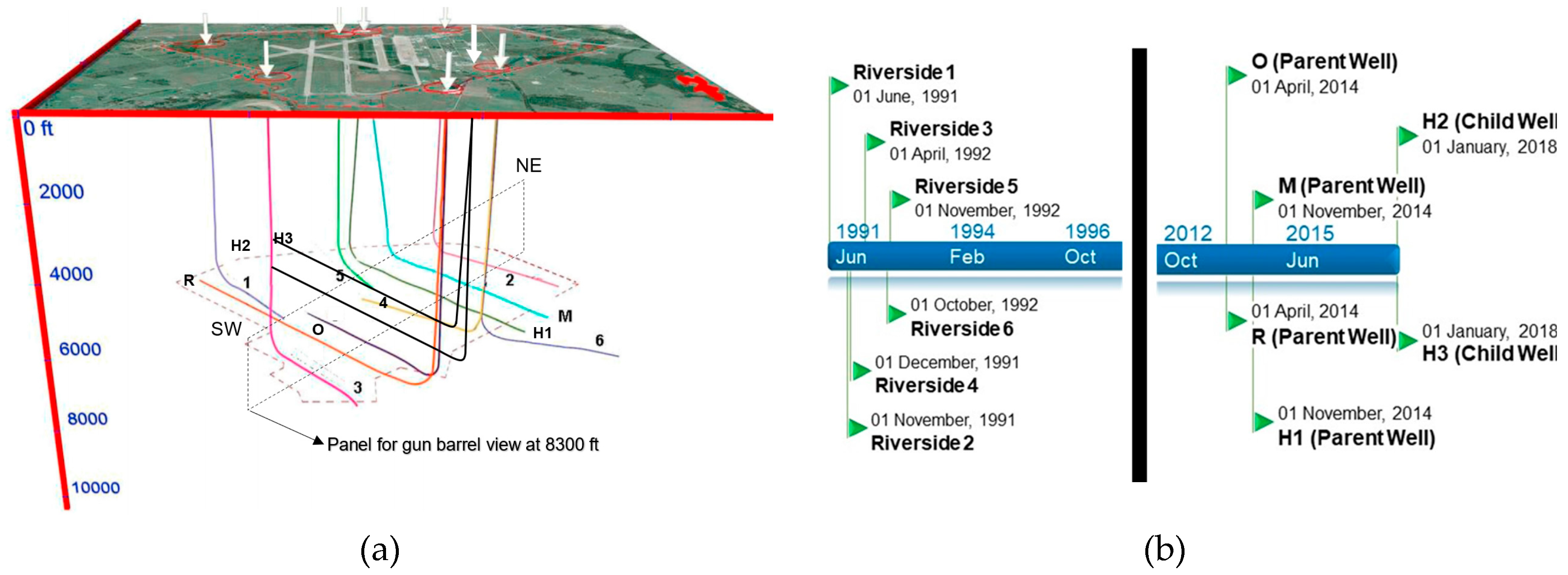
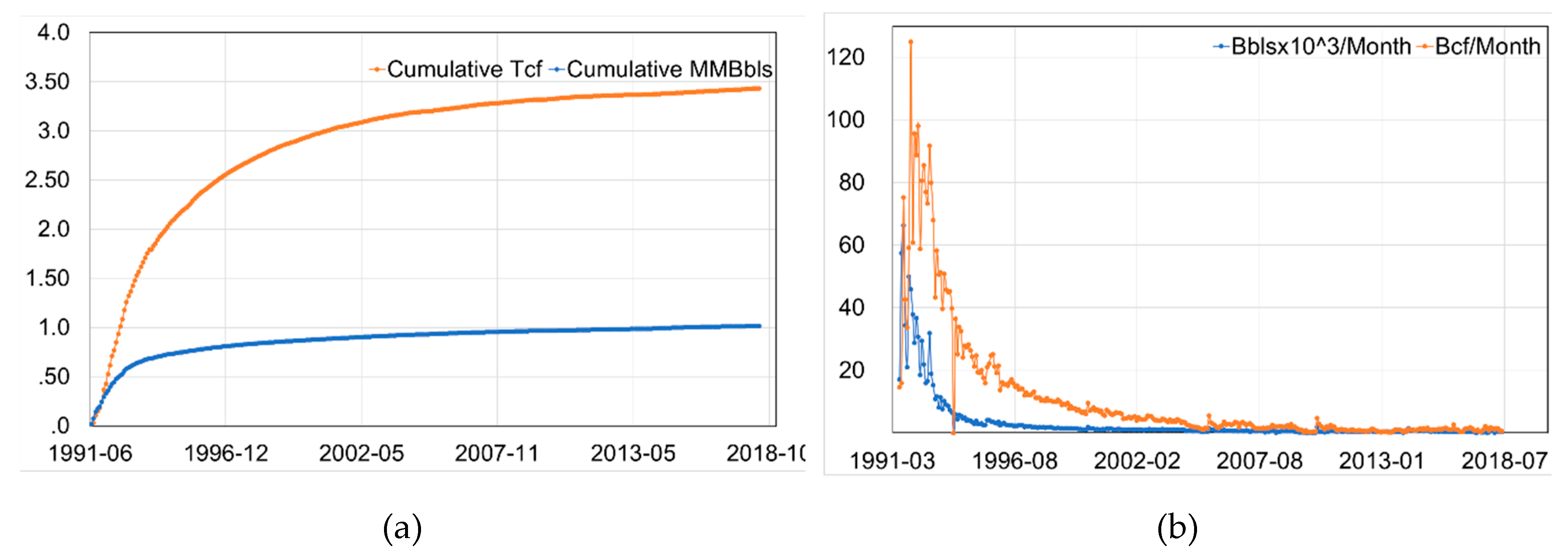
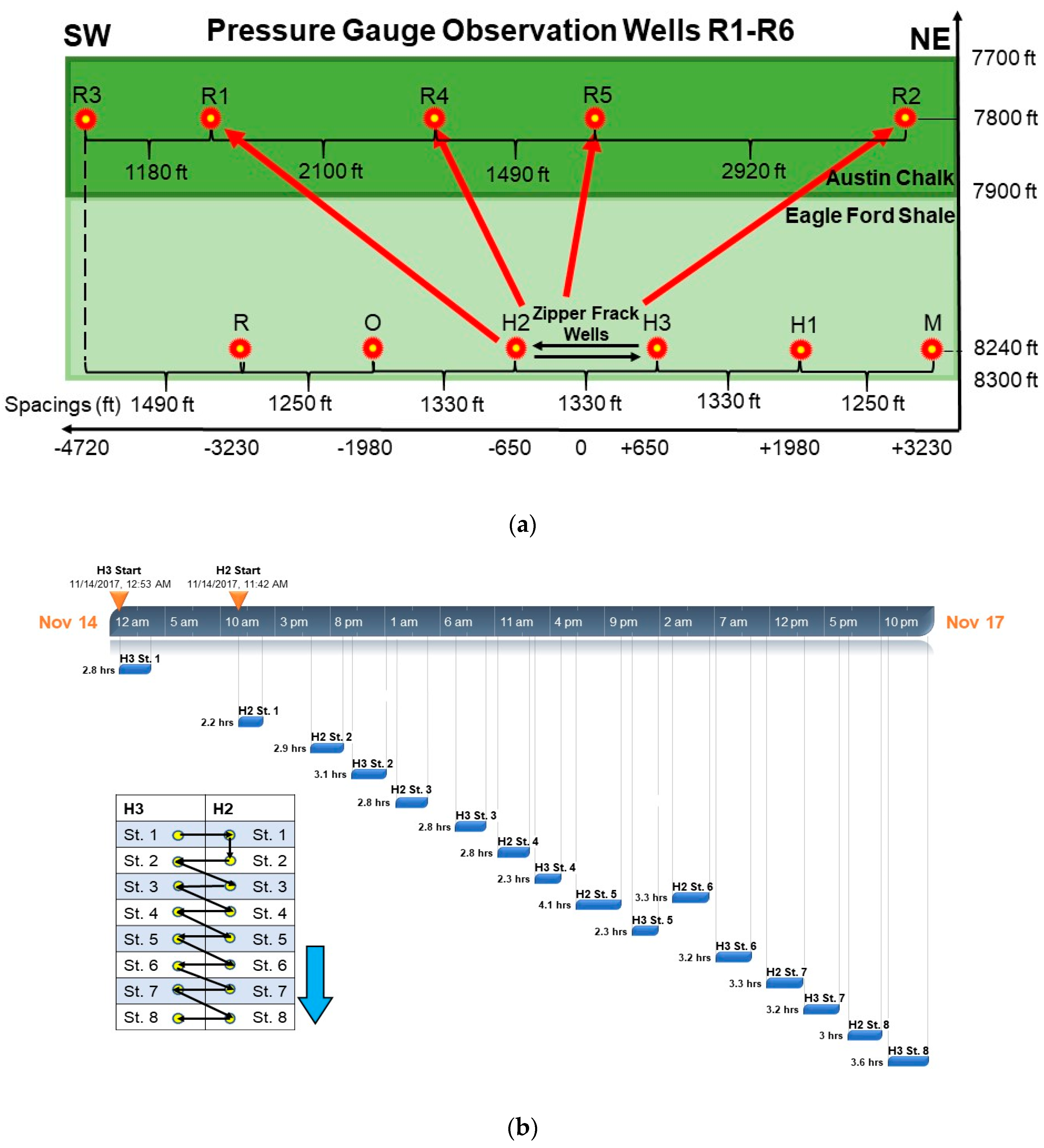
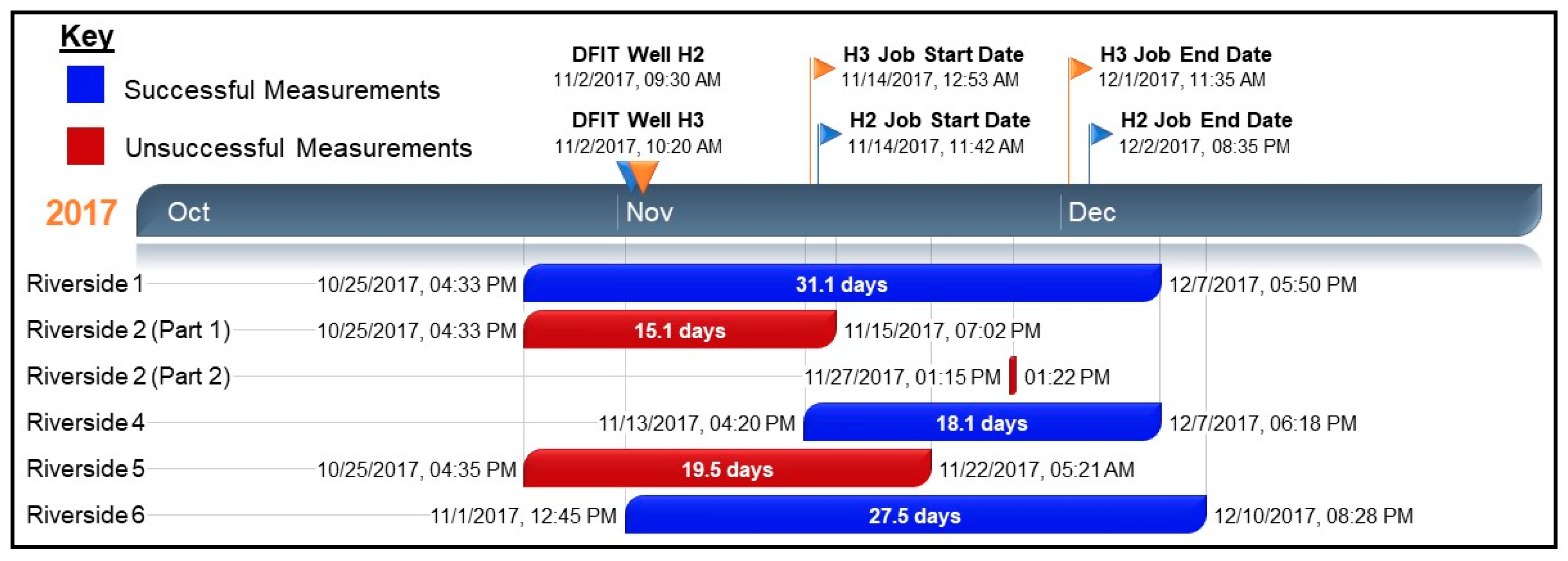
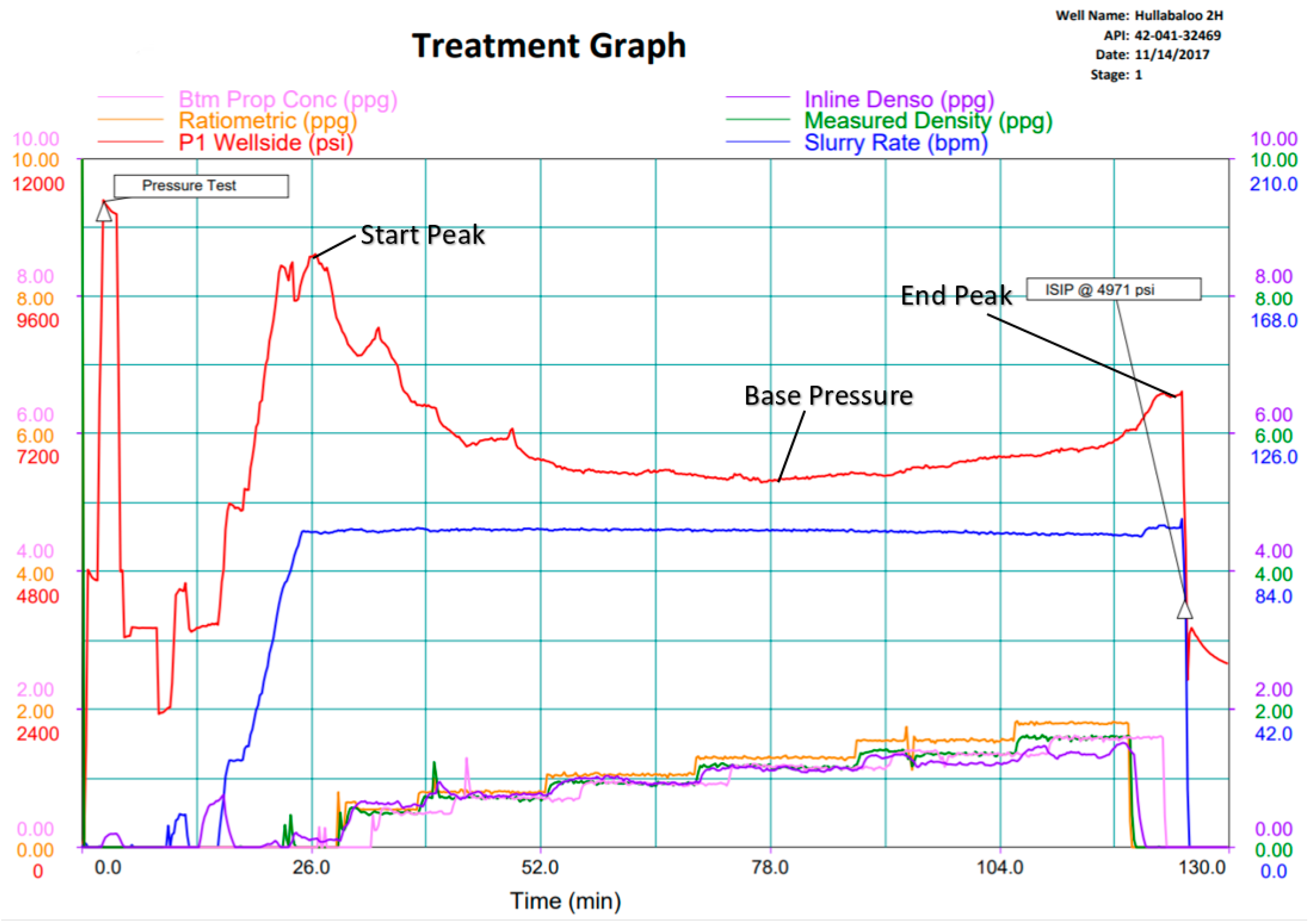
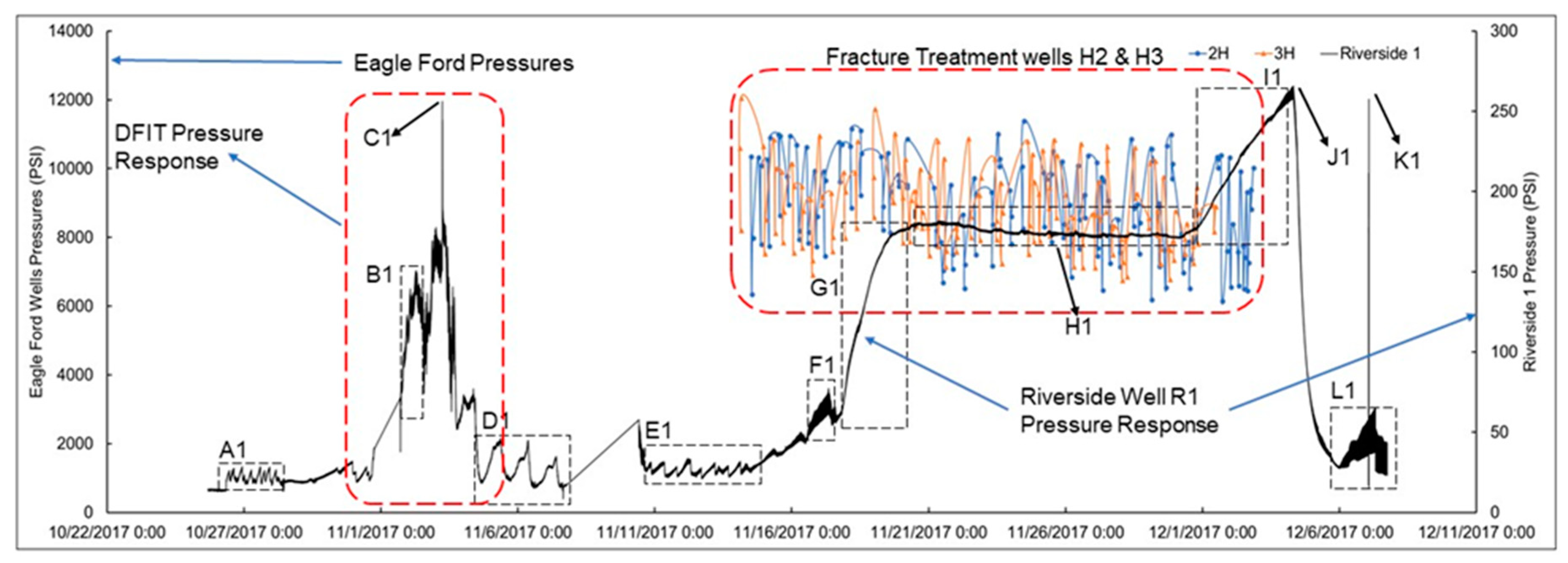
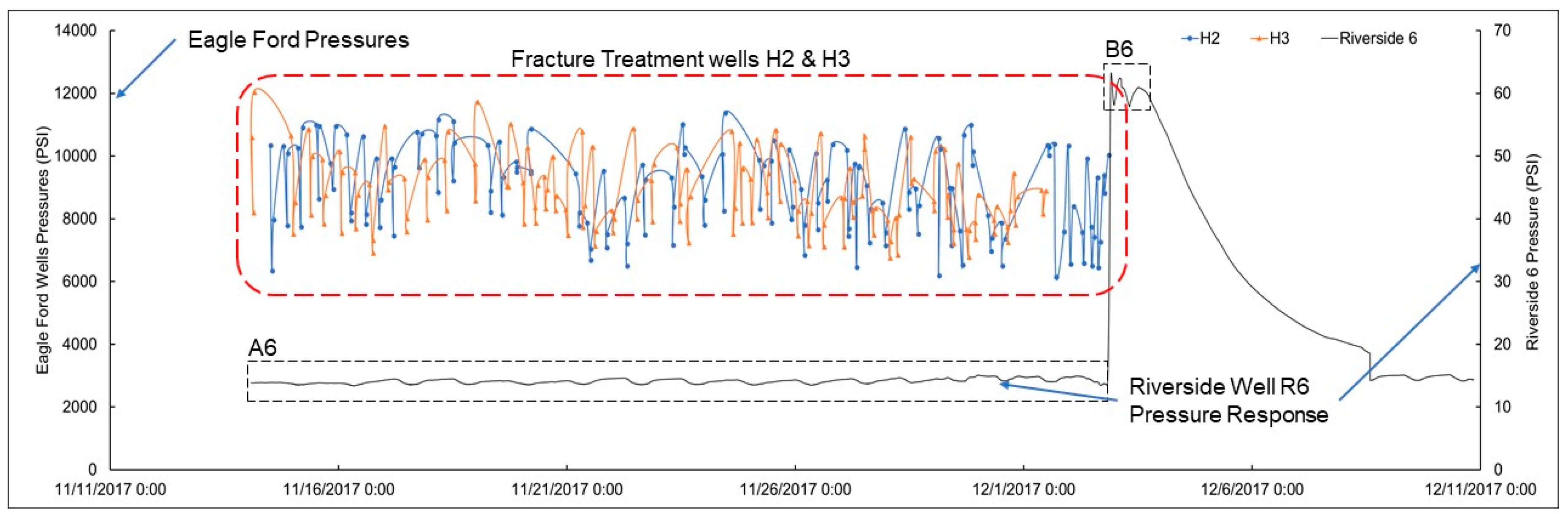
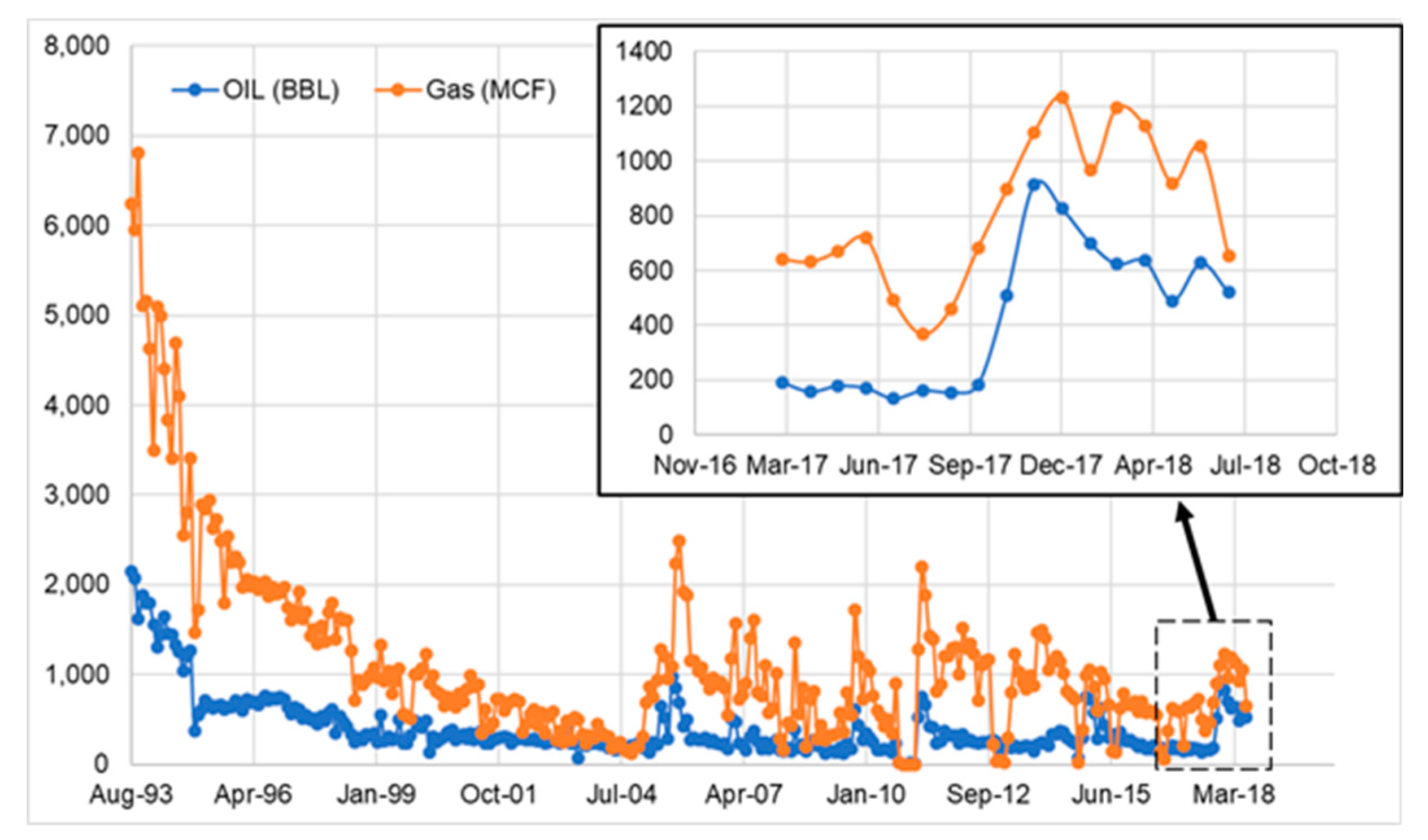
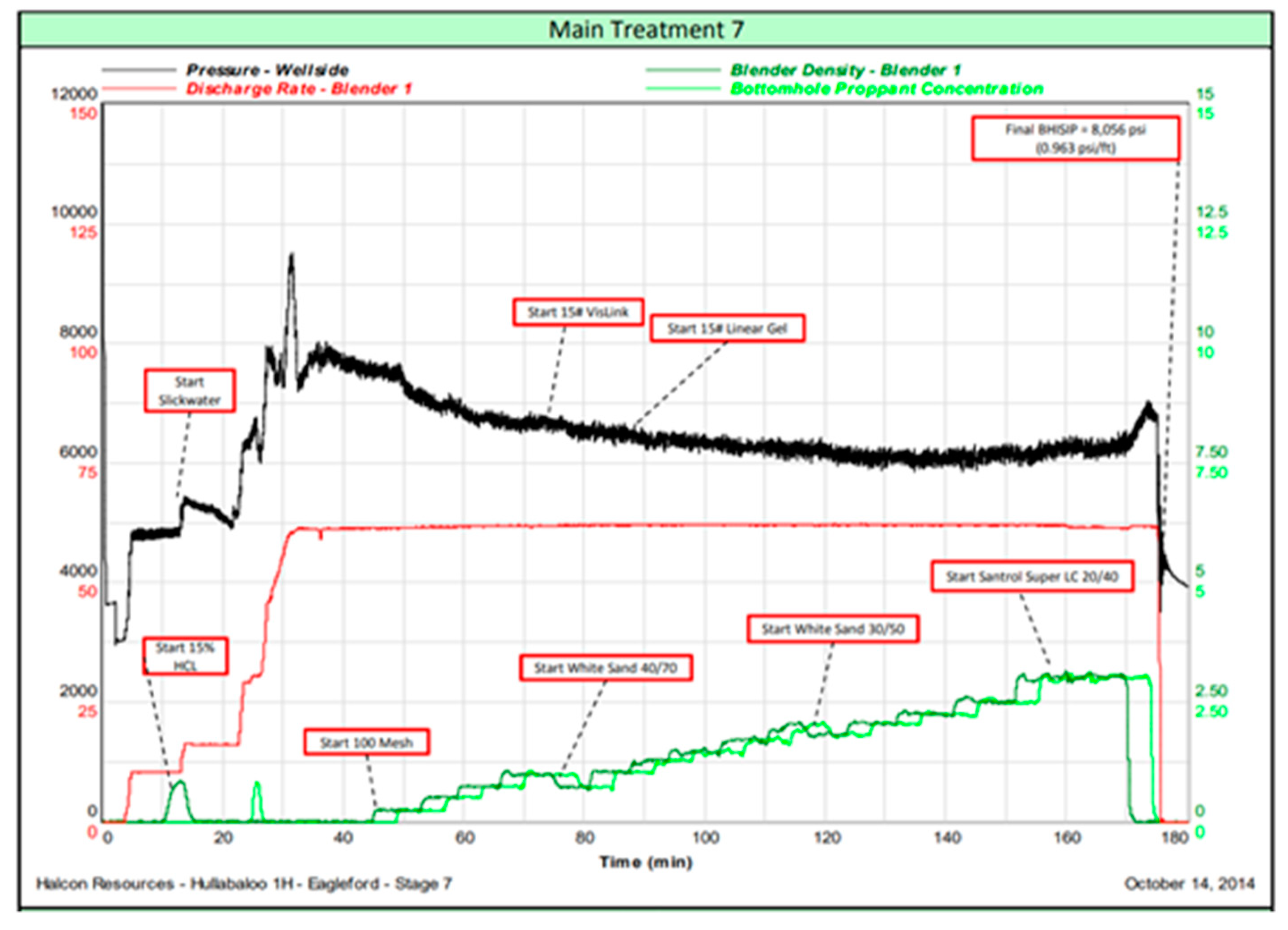
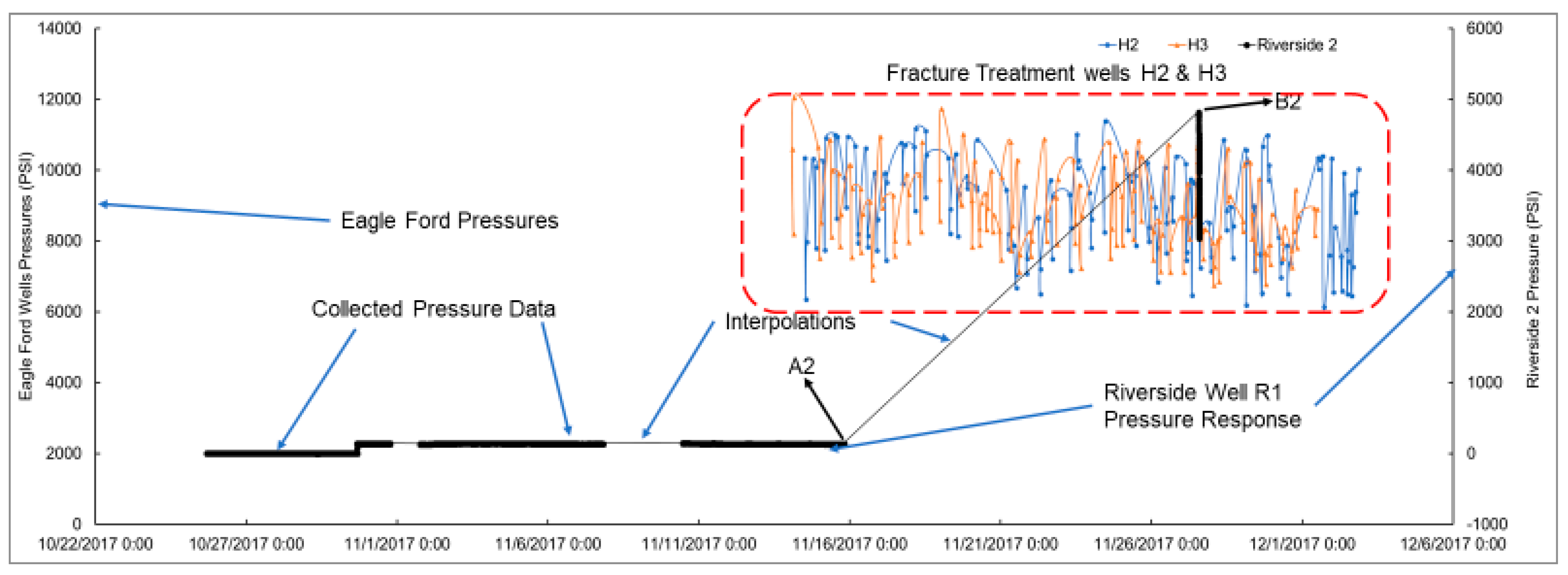
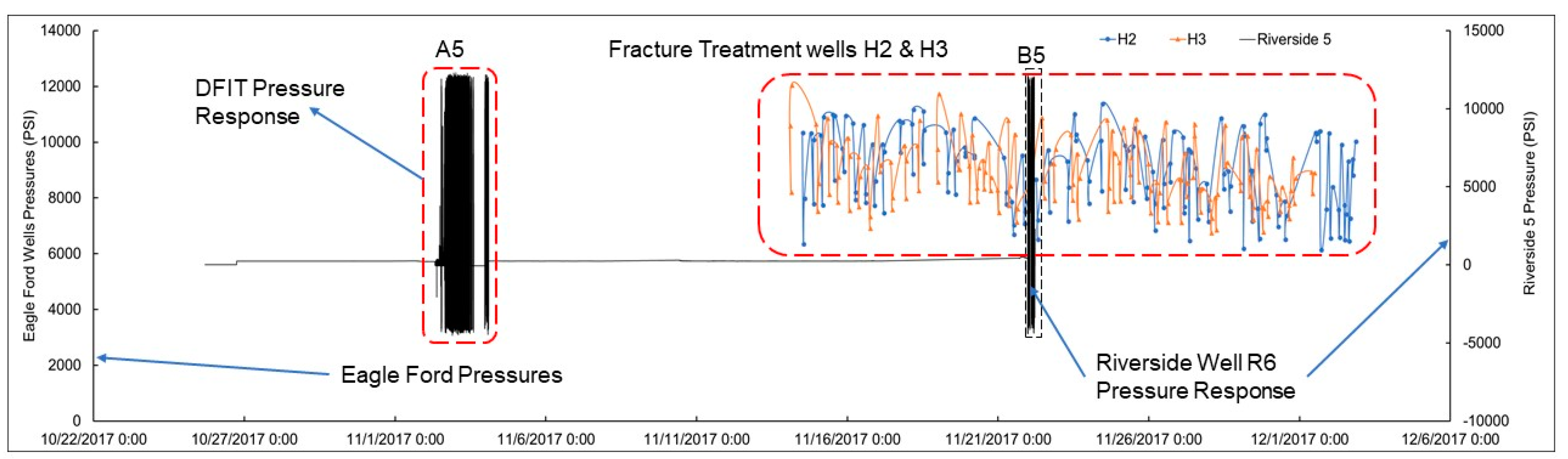