Article

Forecasting Daily Solar Radiation Using CEEMDAN Decomposition-Based MARS Model Trained by Crow Search Algorithm

1
Department of Civil Engineering, Graduate University of Advanced Technology, Kerman 76318-18356, Iran
2
Department of Civil Engineering, Pardisan University, Freidoonkenar 74715-47516, Iran
3
Department of Railroad Construction and Safety Engineering, Dongyang University, Yeongju 36040, Korea
4
Department of Civil Engineering, Tabari University of Babol, Babol 47139-75689, Iran
5
Department of Physical Education, Shahid Bahonar University, Kerman 76169-13439, Iran
6
Department of Land, Water and Environment Research, Korea Institute of Civil Engineering and Building Technology, Goyang 10223, Korea
7
Department of Civil Engineering, Monash University, 23 College Walk, Clayton, VIC 3800, Australia
*
Authors to whom correspondence should be addressed.
Energies 2019, 12(8), 1416; https://doi.org/10.3390/en12081416
Submission received: 25 February 2019 / Revised: 28 March 2019 / Accepted: 4 April 2019 / Published: 12 April 2019
(This article belongs to the Special Issue Modelling and Simulation of Smart Energy Management Systems)

Abstract

:
The precise forecasting of daily solar radiation (DSR) is receiving prominent attention among thriving solar energy studies. In this study, three standalone models, including gene expression programing (GEP), multivariate adaptive regression splines (MARS), and self-adaptive MARS (SaMARS), were evaluated to forecast DSR. A SaMARS model was classified as MARS model when using the crow search algorithm (CSA). In addition, to overcome the limitations of the standalone models, the complete ensemble empirical mode decomposition with adaptive noise (CEEMDAN) was employed to enhance the accuracy of DSR forecasting. Therefore, three hybrid models including CEEMDAN-GEP, CEEMDAN-MARS, and CEEMDAN-SaMARS were proposed to forecast DSR in Busan and Incheon stations in South Korea. The performance of proposed models were evaluated and affirmed that the accuracy of the CEEMDAN-SaMARS model (NSE = 0.878–0.883) outperformed CEEMDAN-MARS (NSE = 0.819–0.818), CEEMDAN-GEP (NSE = 0.873–0.789), SaMARS (NSE = 0.846–0.769), MARS (NSE = 0.819–0.758), and GEP (NSE = 0.814–0.755) models at both stations. Therefore, it can be concluded that the optimized CEEMDAN-SaMARS model significantly enhanced the accuracy of DSR forecasting compared to that of standalone models.

1. Introduction

Due to the negative impacts of fossil fuels on the environment, renewable energy resources have attracted the attention of governments, researchers and industries. Solar energy is a prominent infinite energy source because of its remarkably accessible properties such as radiant light and heat from the Sun, and its applications including electricity generation and air heating/cooling [1]. Recently, solar energy exploitation has become cheaper and more efficient due to the development of various techniques and market competition. Comprehensive understatement of solar radiation is essential for different technological methods of solar energy production as well as the selection of feasible installations in the future [2,3,4]. Solar radiation is spatially and temporarily variable, and therefore site measurements are necessary. However, due to various problems (e.g., lack of instruments and fiscal issues), the authentic DSR are scarce [5,6]. Thus, it is clear that applying efficient methods are important for estimating DSR based on other input variables such as meteorological and geographical variables [7].
In recent decades, data-driven methods, such as artificial neural networks (ANNs) [8], adaptive neuro fuzzy inference system (ANFIS) [9], support vector machine (SVM) [10], M5-model tree [11], multivariate adaptive regression splines (MARS) [12], and gene expression programing (GEP) [13], have been widely applied for energy demand and solar radiation forecasting studies. For instance, Yadav and Chandel [14] used ANNs to perform an exhaustive review of the prediction of solar radiation. They showed the ability of ANNs for solar radiation forecasting based on different case studies. Sozen et al. [15] validated the performance of ANNs for solar radiation prediction based on geographic parameters of Turkey. Dorvlo et al. [16] evaluated two kinds of neural network namely multilayer perceptron (MLP) and radial basis function (RBF). Alsina et al. [17] evaluated the performance of ANNs for the prediction of monthly solar radiation using 45 meteorological stations over Italy. Lou et al. [18] applied a black box model using a boosted regression tree for predicting the diffusion of SR in Hong Kong and Denver. Moreover, Mohammadi et al. [19] employed wavelet transform (WT)-based SVM to enhance the accuracy of standalone SVM. The method combined a firefly meta-heuristic algorithm with support vector regression (SVR) and was designed by Olatomiwa et al. [9] to evaluate the accuracy of developed methods for solar radiation estimation in Nigeria. Antonanzas et al. [20] evaluated SVR performance for mapping solar irradiation using exogenous input variables, whereas Monteiro et al. [21] compared the ability of two models (e.g., ANNs and SVR) to generate photovoltaic power. Chen et al. [22] estimated a solar radiation problem using least-square SVR (LSSVR) based on the atmospheric data at Chongqing meteorological station, China. Salcedo-Sanz et al. [23] also developed an integrated neuro-evolutionary wrapper-based technique for estimating DSR in Queensland, Australia. They used coral reef optimization (CRO) for the feature selection process to access an optimal set of predictor variables using an extreme learning machine (ELM) method.
Nevertheless, various investigations have been accomplished for estimating solar radiation using empirical and conventional methods, but there is an essential challenge to develop a method to overcome non-stationary time series. To address non-stationary problems, several pre-processing approaches (e.g., the principal component analysis (PCA) [24,25], continuous wavelet transform (CWT) [26,27,28], moving average (MA) [29], wavelet multi-resolution analysis (WMRA) [30], maximum entropy spectral analysis (MESA) [31], singular spectrum analysis (SSA) [32,33], and empirical mode decomposition (EMD) [34]) have been used to decompose input/output variables. These techniques are useful tools to resolve the frequency components of input/output time series data by decomposing original datasets into several sub-series, before such datasets are applied in time series estimations.
More recently, complete enhanced EMD with adaptive noise (CEEMDAN) [35] was successfully applied to reconstruct the original input/output variables precisely. It gives a better spectral separation of the intrinsic mode functions at a lower computational cost. Few studies have been accomplished to enhance the model’s performance using CEEMDAN for forecasting different types of data. Zhang et al. [36] investigated and forecast short-term wind speed on the eastern coast of China using CEEMDAN with the flower pollination algorithm (FPA). Prasad et al. [37] used CEEMDAN and EEMD integrated with ELM to improve models’ performance for soil moisture forecasting. They provided that the CEEMDAN-ELM model outperformed the other models for upper layer soil moisture forecasting. Moreover, two-phase integration of ELM and CEEMDAN algorithm was investigated by Wen et al. [38] to predict real-time runoff. They designed a two-phase hybrid model, which utilized CEEMDAN combined with the variational mode decomposition (VMD) method to resolve the frequency of the original datasets in the Yingluoxia watershed, Northwestern China.
This paper presents an integrated model that is designed for coupling CEEMDAN decomposition with data-driven models for improving forecasting accuracy of DSR. In the present research, the original time series is first decomposed by CEEMDAN for better frequency resolution. The main contribution of this study is that, for the first time, an integrated CEEMDAN algorithm with data-driven models (e.g., GEP, MARS, and SaMARS) is proposed to supply prominent frequency-based input information to forecast DSR. The proposed integrated models are applied at Busan and Incheon meteorological stations in South Korea. Then, it is benchmarked and evaluated with standalone models (e.g., GEP, MARS, and SaMARS) using several statistical criteria.

2. Data Collection

In this study, meteorological data were collected from two weather stations, namely Busan (Longitude, 129°03′ E; Latitude, 35°10′ N; Altitude, 69.2 m) and Incheon (Longitude, 126°70′ E; Latitude, 37°45′ N; Altitude, 21.12 m), in South Korea (Figure 1). These stations are operated and maintained by the Korea Meteorological Administration (KMA). The weather data consist of 16 years (from 2000 to 2016) covering daily records of air temperature (TA), sunshine duration (SD), relative humidity (RH), vapor pressure (VP), sea-level pressure (SLP), pan evaporation (PE), and daily solar radiation (DSR).
Generally, the accessibility of a long-term measured dataset is of particular importance for an accurate estimation of DSR. Furthermore, the accuracy of models for DSR forecasting is affected by the quality of DSR time series data. In measured DSR data, there have been some contradictions and abnormalities in the values mainly because of malfunctioning instruments [6]. After the data sorting, every missing value was replaced with interpolated values by means of various approaches for time series analysis. In addition, this method provides that if there are some missing days or a datum is incorrect, it can be replaced with the means of two nearest non-missing values [39].
In the present study, the data were divided into two sub-sets: the first for calibration and the second for validation. Hence, the first data cover the period from 1 January 2000 to 31 December 2012, while the second data include the period from 1 January 2013 to 31 December 2016. The calibration dataset was applied for creating and statistically analyzing a suitable model, while the second data were used to validate the accuracy and efficiency of selected models. Table 1 presents the statistical parameters related to climatic variables in the selected stations.

3. Methodology of CEEMDAN and Data-Driven Models

3.1. Complete Ensemble EMD with Adaptive Noise (CEEMDAN)

The EEMD introduced by Wu and Huang [40] is an adaptive technique for representing non-linear and non-stationary signals as the sum of signal elements with modulated parameters of domain and frequency; a noise-assisted analysis method is given by the popular EMD [41]. The EMD is as a self-adaptive decomposition model, without initial knowledge of the number and nature of intrinsic mode functions (IMFs) and is embedded in the data [40,41]. However, research has shown that EMD has a limitation regarding mode mixing [40]. Mode mixing is either a single IMF including vast disparate scale elements or a similar scale element, which exist in IMFs [42]. EEMD is introduced as an enhanced procedure for overcoming the mode mixing problem in EMD.
Even if EEMD solves this problem, a finite average, the Gaussian white noise added using the EEMD may not be canceled after resulting in an error of reconstruction. The complete ensemble EMD with adaptive noise (CEEMDAN) is defined as an enhanced EEMD approach. However, there is a high level of computational cost (associated with the exhaustive search) and includes residual noise in the EEMD method. An increase in the number of trials can potentially increase the number of sifting process. A CEEMDAN was employed for declining the trials number while keeping the capacity for resolving the problem of mode mixing [43].
In brief, the CEEMDAN steps are as follows:
(1) This method applies for computing the first mode function as following Equation (1).
IMF 1 ¯ ( t ) = 1 N j = 1 N IMF 1 j ( t )
The first residue is also given as following Equation (2).
r 1 ( t ) = x ( t ) IMF 1 ¯ ( t )
(2) Determine emd(t) as the kth IMF element using the EMD method and decompose the sequence r1(t) + p1emd1(nj(t)) to reach the second component of IMF.
IMF 2 ¯ ( t ) = 1 N j = 1 N e m d 1 ( r 1 ( t ) + p 1 e m d 1 ( n j ( t ) ) )
A residual signal is provided.
r 2 ( t ) = r 1 ( t ) IMF 2 ¯ ( t )
(3) Likewise, in the previous step, the kth residual signal is estimated.
r k ( t ) = r k 1 ( t ) IMF k ¯ ( t )
The component of k + 1th IMF is then derived.
IMF k + 1 ¯ ( t ) = 1 N j = 1 N e m d 1 ( r k ( t ) + p k e m d k ( n j ( t ) ) )
(4) Iterate these steps while the residual signal is reached. Suppose, there are L components of IMF. Hence, the original sequence can be computed as:
y ( t ) = i = 1 L IMF 1 ¯ ( t ) + r ( t )
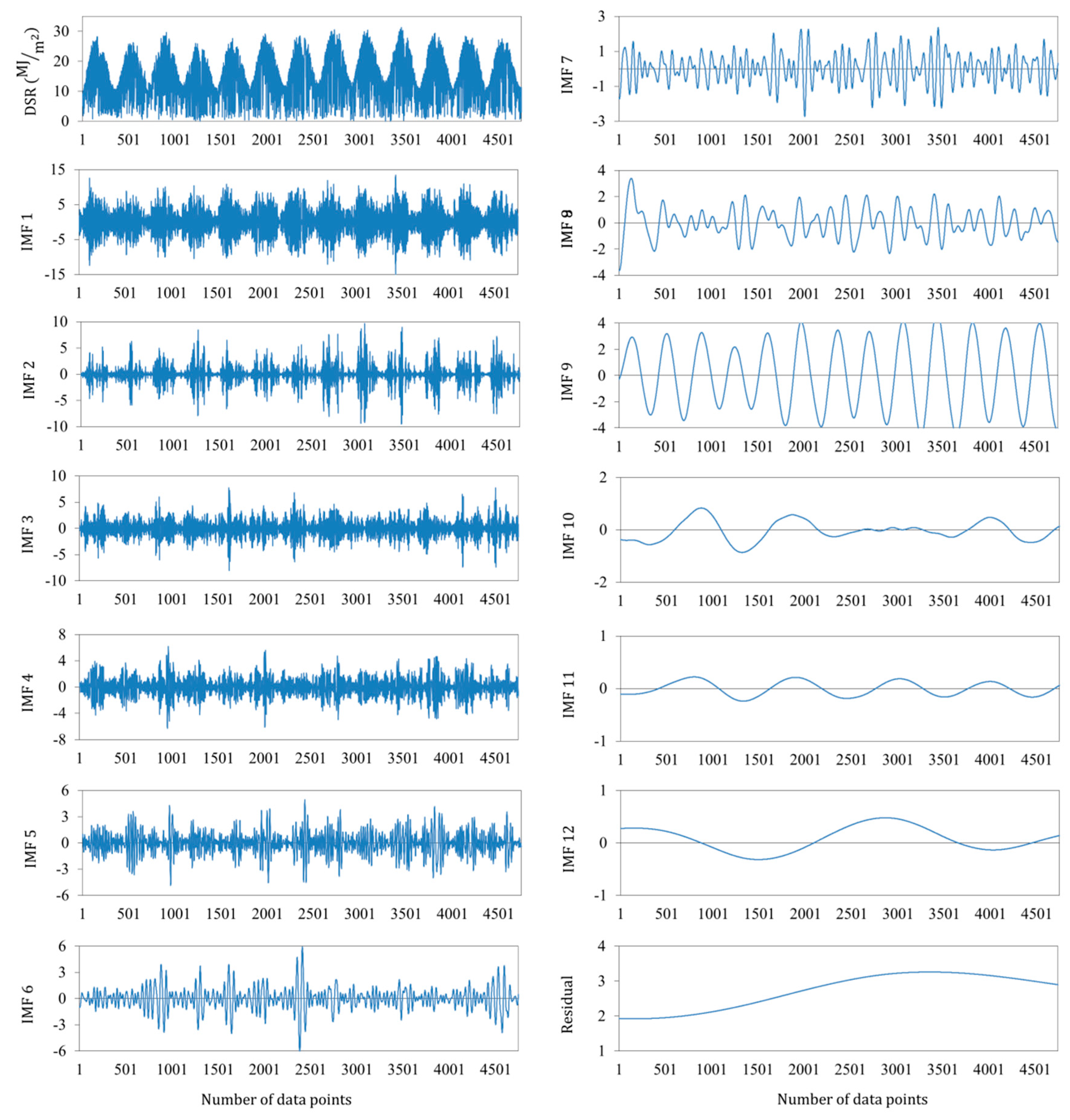
where r(t) is the final residual signal. In this study, the optimum standard deviation is equal to 0.5 and L = 500. According to Figure 2, the original DSR data series was decomposed using CEEMDAN.

3.2. Gene Expression Programing (GEP)

GEP model is a subset of GP introduced by Ferreira [44], and consists of five components namely the terminal set, terminal condition, function set, control parameters and fitness function. The GEP model applies character strings of fixed lengths for solving the problems, while parse structures of trees with various lengths are used. Moreover, the GEP model can develop complicated non-linear programs by several subprograms because of its multigenic system. A gene of GEP model is created by two symbol types: the first symbol is fixed length variables and another is constants which is known as terminal set (e.g., {a, b, c, 6}) and some operations as the function set (e.g., {+, −, log}) [45]. The generated chromosomes by the GEP model indicate parse trees which are used for reading the encoded information at the strings using Karva language. After that, these chromosomes can be described as expression trees (branched structures). The nodes recorded between the root and the deepest layers can be utilized for inverse expression tree transformation to the Karva expression (K-expression) for generating the primary string [46]. In this way, the K-expression length should be either equal or less than the GEP gene [47].
A GEP model begins while the chromosomes related to fixed lengths are generated randomly in each. When these chromosomes are revealed, all individuals are investigated in case of fitness. The individuals are subsequently determined to reproduce based on their fitness. In every generation, this process is iterated until a solution is found. In this method, genetic operations (e.g., mutation and crossover) are also used to convert population [44,45].

3.3. Multivariate Adaptive Regression Splines (MARS)

A MARS model is a sort of non-linear model, which was introduced by Friedman [48]. Regarding this approach, there is no presumption about basic function relations among input/output variables. The segment endpoints, which are defined as nodes, can determine the endpoint at each region [49,50].
The MARS model builds basis functions using the step searching means. In addition, the MARS model is built using a two-step method. At first, functions are added until probabilistic nodes are found (primary phase). The second step involves removing the minimum real terms (secondary phase). Suppose y is a deterministic output and X = ( X 1 , …, X p ) is the input variable. Thus, it can be said that data are obtained from an unknown “real” model. Consequently, the response is as follows [51]:
y = f ( x 1 , , x p ) + e = f ( x ) + e
where, e is the error distribution. The MARS model is recruited to approximate function f by means of the basis functions (BFs). In fact, BFs are referred to splines (smooth polynomials) including piecewise-cubic and piecewise-linear functions. Equation (9) is extracted from the MARS model when alinear combination of BFs and their mutual relations is created [52],
f ( x ) = β 0 + m = 1 M β m λ m ( x )
where, each λ m ( x ) is a BF which might be a spline function or product of two or more spline functions. Coefficients β are constant values and can be evaluated by least squares (LS) method.
The MARS model is known as one of data-driven models. Firstly, the primary method is accomplished for training data. By cutting off the β0 and basis pair, one model is built that has the maximum reduction of training error. The next pair is added to the current model on the basis of the M BFs as follows (10) [53],
β ^ M + 1 λ 1 ( X ) m a x ( 0 , X j t ) + β ^ M + 2 λ 1 ( X ) m a x ( 0 , t X j )
where the LS technique is used for estimating β. In addition, mutual interactions among the BFs in the model are carefully considered when new BF is added to the model space. Then, BFs are added into the model to achieve the maximum specified number of terms that bring about a perfect fitness model. After that, a backward removal discipline is applied to decrease the number of terms. The main aim of this deletion approach is finding an optimal number of parameters (terms) by getting rid of the unessential variables.

3.4. Crow Search Algorithm (CSA)

Crows are capable of memorizing faces, communicating in sophisticated ways, as well as hiding and retrieving food during different seasons. These characteristics of crows allow them to discover where other crows hide their food and steal it when the owner leaves. Considering this, Askarzadeh [54] proposed a novel evolutionary algorithm, named crow search algorithm (CSA), to solve complex optimization issues. This algorithm follows given principles:
(1) Crows live in the flock form; (2) They memorize the places that they hid their food; (3) They follow each other to conduct thievery, and (4) They preserve their caches from being pilfered using a probability.
Similar to other optimization-based algorithms, CSA starts the optimization process with a dimensional environment compared to the population of crows. The crow number is N and the position i of crow at each iteration in the search space is computed using a vector x i , i t e r = [ x 1 i , i t e r , x 2 i , i t e r , , x d i , i t e r ] where i = ( 1 ,   2 ,   ,   N ) and i t e r = ( 1 ,   2 ,   ,   i t e r m a x ) . itermax is the number of maximum iterations.
There is a parameter in CSA named awareness probability which its role is to balance the intensification and diversification [55] to increase the intensification using small values for awareness probability by searching on a local space and by increasing the awareness probability value; CSA can tend to determine the searching space on the global scale. CSA implementation for optimization can be briefly explained as [54]:
  • Defining the optimization problem with all of its constraints, determining the decision variables and setting the CSA parameters, flock size (N), the flight length (fl), maximizing the iteration number (itermax), and the awareness probability (AP).
  • Initializing the position and memory in a d-dimensional search space randomly for crows according to Equations (11) and (12). Each crow can be suitable solution for the problem and d indicates the quantity of the decision variables.
    Position = [ x 1 1 x 2 1 x d 1 x 1 2 x 2 2 x d 2 x 1 N x 2 N x d N ]
    Memory = [ m 1 1 m 2 1 m d 1 m 1 2 m 2 2 m d 2 m 1 N m 2 N m d N ]
  • Evaluating the fitness function for each crow by placing the decision variables into the objective function.
  • Generating new positions as follows: crow i can generate a new situation and select ones among other cows (crow j) randomly and follows it to discover crow j’s hidden food source.
  • The possibility of the new positions for all crows is checked as follows: If new position of crows is possible, the position of that crow is updated. Else, the crow remains in the current situation and new position is not generated for that crow.
  • The fitness function for the new position of each crow is evaluated.
  • The crows update their memory by Equation (13):
    m i , i t e r + 1 = { x i , i t e r + 1 f ( x i , i t e r + 1 )   is   better   than   f ( m i , i t e r ) m i , i t e r   otherwise
    where f(.) is an objective function, xi,iter is the position of crow i in iteration, iter and mi,iter are the memory of crow i in iteration iter. The termination criterion is checked (repeat steps 4–7 until itermax). Eventually, the best memory position based on the objective function value is considered as the optimum solution.

3.5. Self-Adaptive Multivariate Adaptive Regression Splines (SaMARS)

In computer science, a careful choice of parameters belonging to data-driven models, such as ANN, ANFIS, and SVM, is a crucial step to attain outstanding performance in modeling processes. For instance, the number of hidden nodes and layers (both discrete) or the weights and biases are the necessary parameters, which need to be optimized in an ANN model. Even if the model provides appropriate consequences to an addressed problem, its parameters due to incorrect choices may result in a worse performance than expected. The common technique to find desirable parameters is to combine prior experiences with a limited heuristic search of optimal solutions which takes a lot of time for the user and might not address the issue.
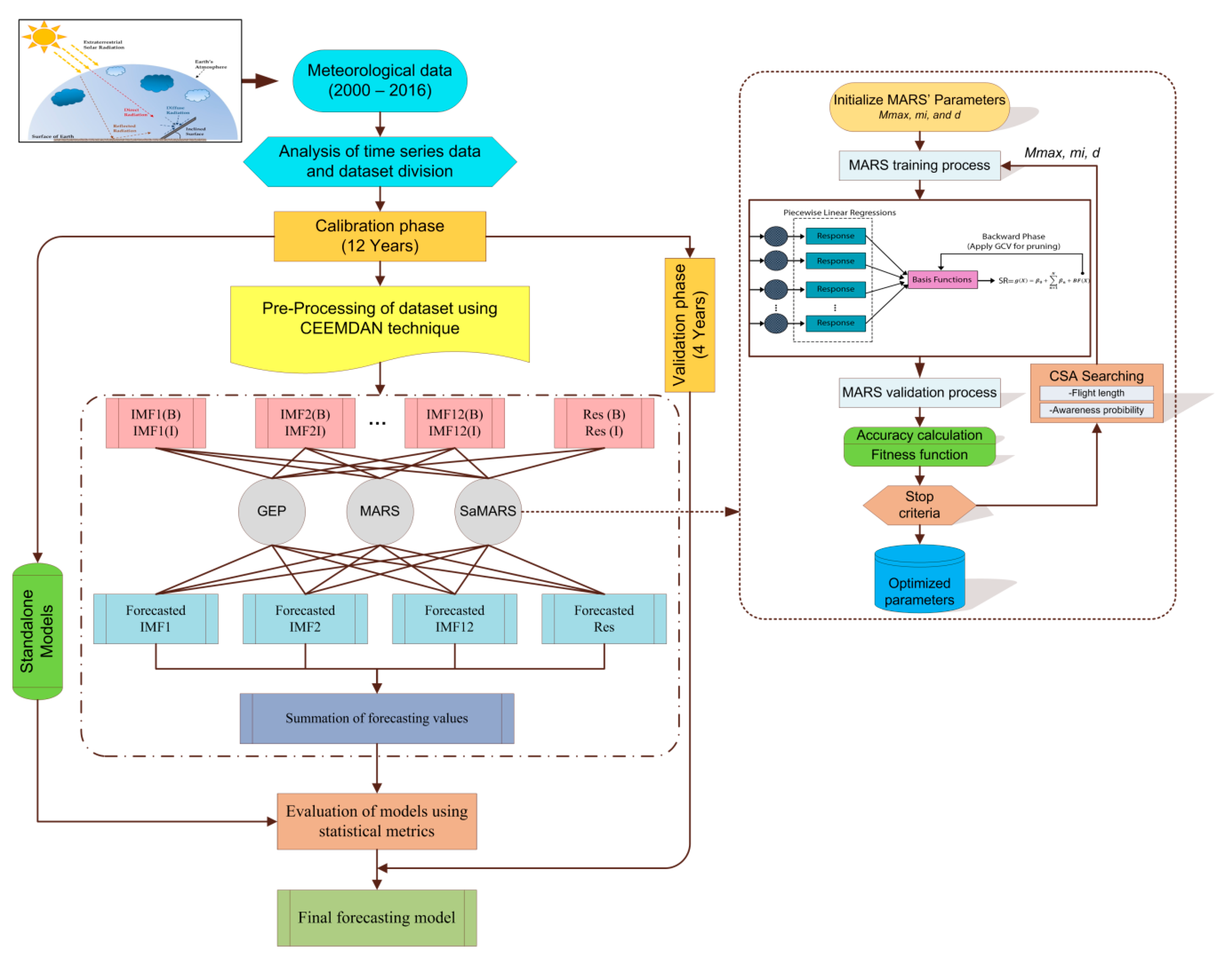
In addition, the MARS model depends on its parameters containing penalty parameter d, maximum BF Mmax, and interaction mi. Using MARS model, however, makes it difficult to find optimal parameters simultaneously due to its large range of choices, which appropriate parameters can significantly improve MARS model’s forecasting accuracy, and also suitable values can still lie outside suggested ranges. Thus, this study presents SaMARS model as a helpful method to assist users encounter this challenging issue (Figure 3). Firstly, the MARS model is deployed for handling the underlying function. A new MARS method is created based on each set of values of the CSA-provided parameter. CSA’s greedy selector compares the quality of proposed model quality regarding evaluation of fitness function. After the calibration processing, the MARS model is employed to verify the validation dataset. The following objective function is applied to check the fitness function of the model:
f = E c a l i b r a t i o n + E v a l i d a t i o n
where, Ecalibration and Evalidation indicate calibration and validation error, respectively. In Equation (14), root mean square error (RMSE) is applied as the estimation error index. It is worth pointing out that the fitness function in Equation (14) represents the trade-off between complexity complexity and generalization of model. Due to the fact that the over-fitting occurs more in the training stage, the combination of calibration and validation errors can build a model to balance optimally with minimum calibration error and model generalizability. In the second step, CSA conducts the search for selecting the best parameter values, containing: Mmax, mi, and d. Once the stop criterion is satisfied, the optimization process is terminated. In this work, a generator number is used as the stop criterion. Prior to reaching the certain generation number, the model is underway. Finally, the optimal forecasting model with the best parameter settings is found when the stop criterion is performed. In other words, the training process of SaMARS has been completed and is ready to forecast DSR using testing data).

4. Model Performance

The accuracy and reliability of the proposed models need to be evaluated and assessed. Therefore, several statistical criteria were employed as follows:
  • Root mean square error (RMSE)
    RMSE = 1 n i = 1 n [ DSR o b s DSR f o r ] 2
  • Relative root mean square error (RRMSE)
    RRMSE = RMSE 1 N i = 1 N DSR o b s
  • Mean absolute error (MAE)
    MAE = 1 N i = 1 N | DSR o b s DSR f o r |
  • Nash-Sutcliffe efficiency (NSE)
    NSE = 1 i = 1 n [ DSR o b s DSR f o r ] 2 i = 1 n [ DSR o b s DSR ¯ o b s ] 2
  • Willmott’s index of agreement (WI)
    WI = 1 [ i = 1 n ( DSR o b s DSR f o r ) 2 i = 1 n ( | DSR f o r DSR ¯ o b s | + | DSR o b s DSR ¯ o b s | ) 2 ]
  • Legates-McCabe’s index (LMI)
    LMI = 1 [ i = 1 n | DSR f o r DSR ¯ f o r | i = 1 n | DSR o b s DSR ¯ o b s | ]
    where DSR o b s and DSR f o r are the measured and forecasted DSR values; DSR o b s ¯ and DSR f o r ¯ indicate the observed and forecasted mean values of DSR; and N is the number of DSR data points. The first criterion, RMSE [Range = (0, +∞); Ideal value = 0] provides the standard deviation of estimating errors; and MAE [Range = (0, +∞); Ideal value = 0] gives an information about the average discrepancies between observed and forecasted values. Both RMSE and MAE criteria are known as the absolute error measures [37]. In addition, RRMSE [Range = (0, +∞); Ideal value = 0] is an adequate criterion when comparing models of different stations. NSE [Range = (−∞, 1); Ideal value = 1] can be applied for evaluating the capability of hydrological approaches. The highest value of NSE indicates a perfect fit between measured and forecasted DSR. A negative value of NSE presents that the proposed model can perform worse than the mean value of time series dataset [56]. Moreover, WI [Range = (0, 1); Ideal value = 1] is a standardized error value of model prediction. Both criteria (e.g., NSE and WI) are sensitive to outliers because of the squaring of difference terms [37,57]. However, LMI [Range = (−∞, 1); Ideal value = 1] is not inflated using the squared values and is not sensitive to outliers [58].

5. Results and Discussion

In this study, hybrid forecasting models (i.e., CEEMDAN-GEP, CEEMDAN-MARS, and CEEMDAN-SaMARS) are designed using MARS model with CEEMDAN to eliminate non-stationary time series. The efficiency and capability of the proposed hybrid models are compared with three standalone models (e.g., GEP, MARS, and SaMARS) for DSR forecasting in Busan and Incheon stations, South Korea. Figure 3 indicates the main steps of proposed models for enhancing the model’s performance. Also, the design parameters of GEP and MARS models for calibration at Busan and Incheon stations are presented in Table 2.

5.1. Implementation of CEEMDAN Based Models

In this study, DSR was selected as the target variable based on the different input variables including vapor pressure (VP), air temperature (TA), relative humidity (RH), sea-level pressure (SLP), pan evaporation (PE), and sunshine duration (SD).
Firstly, the meteorological input variables were classified as calibration (from 2000 to 2012) and validation (2013 to 2016) dataset. In the second step, the datasets of calibration and validation phases were separately decomposed into various components (sub-series) and one remaining value (residual). The decomposition of time series dataset into twelve IMFs (from IMF1 to IMF12) and one residual component is provided in Figure 2. Then, the GEP, MARS, and SaMARS models were employed as estimation approaches to estimate each decomposed IMF and residual component, and finally, the estimated decomposed IMFs and residual values using the proposed models were aggregated to generate DSR time series to calculate each component using the same sub-series (IMF1) of six input variables, respectively.
To summarize, the hybrid forecasting models (i.e., CEEMDAN-GEP, CEEMDAN-MARS, and CEEMDAN-SaMARS) apply the conceptual idea of “decomposition and ensemble”. The decomposition and ensemble features can simplify the estimation task and formulate a consensus predicting the original dataset, respectively.

5.2. Standalone and Hybrid GEP Models

Results of the GEP and CEEMDAN-GEP models for forecasting DSR in both stations are presented in Table 3. It can be found from Table 3 that the accuracy of the CEEMDAN-GEP model is better compared with the GEP model based on RMSE, RRMSE, MAE, NSE, WI, and LMI values.
At Busan station, the forecasted values of DSR using the GEP model have RMSE = 2.992 (MJ/m2), RRMSE = 0.189, MAE = 2.402 (MJ/m2), NSE=0.814, WI = 0.955, and LMI = 0.585, while the CEEMDAN-GEP model produces the forecasted values with RMSE = 2.514 (MJ/m2), RRMSE = 0.171, MAE = 1.995 (MJ/m2), NSE = 0.873, WI = 0.974, and LMI = 0.654 in the validation phase.
At Incheon station, the CEEMDAN-GEP gave more accurate results compared with the GEP model. That is, the CEEMDAN-GEP model could forecast DSR values with higher accuracy (RMSE = 2.862 (MJ/m2), RRMSE = 0.192, MAE = 2.324 (MJ/m2), NSE = 0.789, WI = 0.952, and LMI = 0.564) compared with the GEP model (RMSE = 3.086 (MJ/m2), RRMSE = 0.211, MAE = 2.501 (MJ/m2), NSE = 0.755, WI = 0.944, and LMI = 0.528) in the validation phase. In brief, the CEEMDAN-GEP model was superior to GEP for DSR forecasting in both stations.
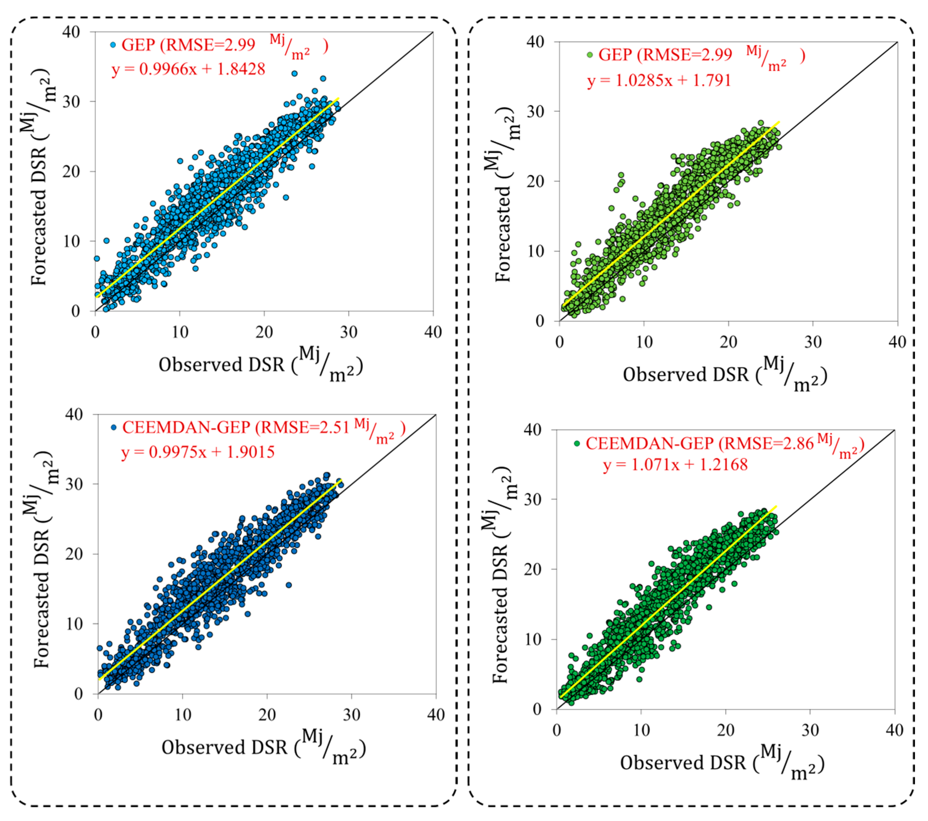
Scatterplots between observed and forecasted DSR values for both stations in the validation phase are presented in Figure 4.
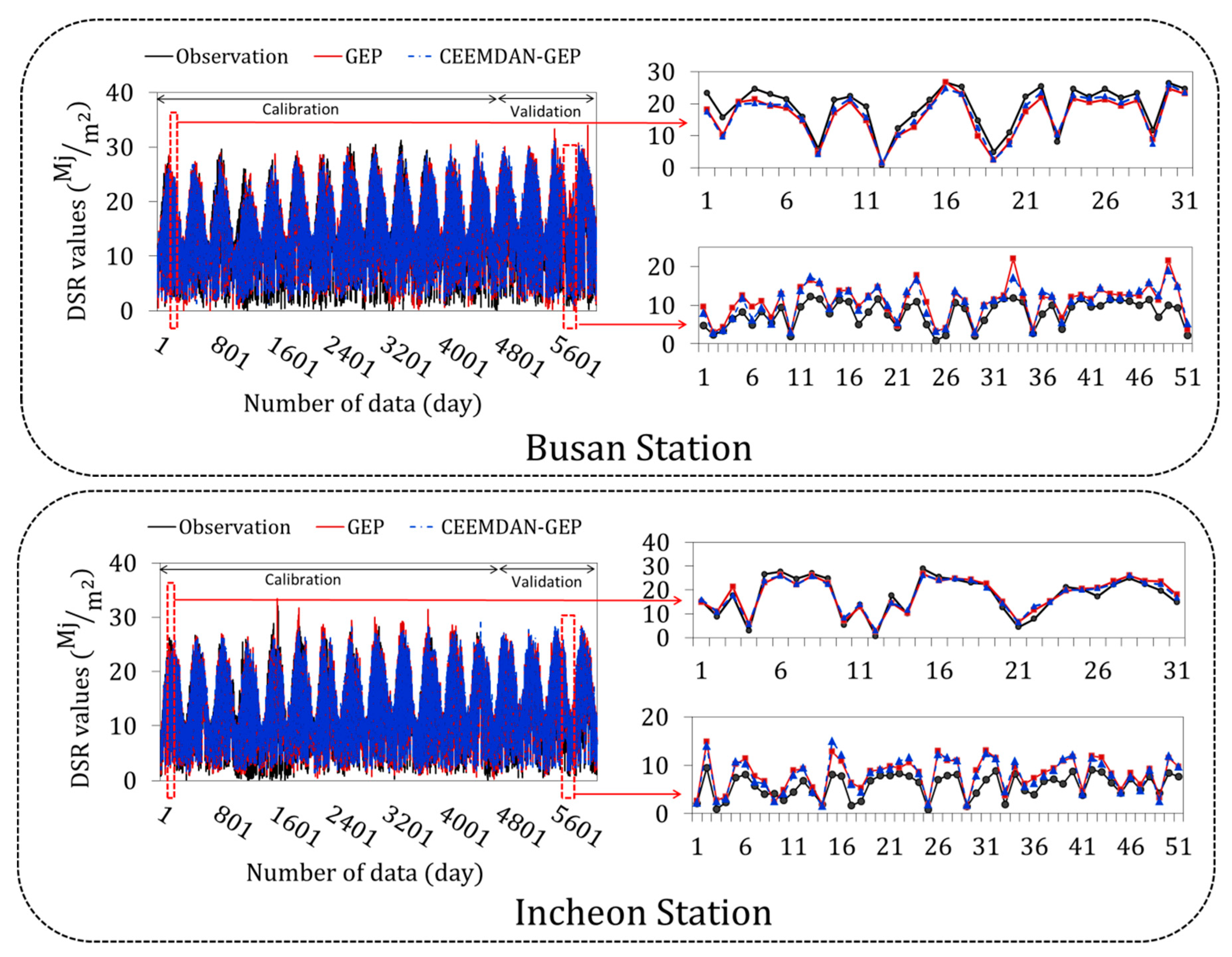
It can be seen from the scatterplots that the CEEMDAN-GEP model’s best-fit lines in the validation phase between the estimated (y) and the observed (x) values are closer to the ideal line (y = x). Figure 5 shows that time-series plots between observed and forecasted DSR for calibration and validation phases in both stations, the CEEMDAN-GEP outperforms GEP model for DSR forecasting in both stations.

5.3. Standalone and Hybrid MARS Models

Based on Table 4, the CEEMDAN-MARS model could forecast DSR with better precision compared with MARS model for calibration and validation phase at Busan station.
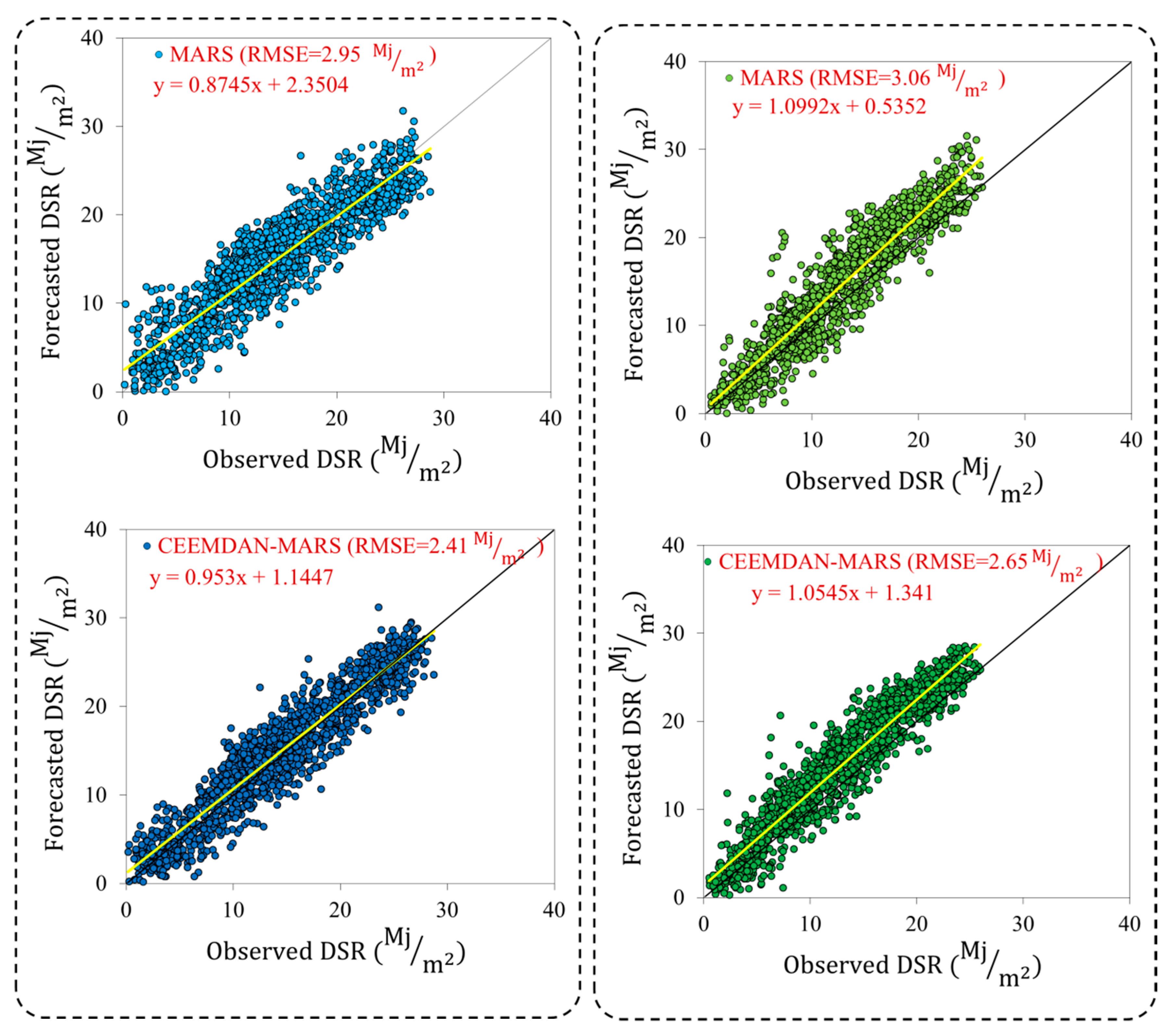
For the validation phase, the CEEMDAN-MARS model showed optimal values with RMSE = 2.412 MJ/m2, RRMSE = 0.166, MAE = 1.983 MJ/m2, NSE = 0.879, WI = 0.969, and LMI = 0.667 compared with the MARS model (RMSE = 2.951 MJ/m2, RRMSE = 0.207, MAE = 2.437 MJ/m2, NSE = 0.819, WI = 0.951, and LMI = 0.581) at the Busan station. This illustrates the ability of the CEEMDAN-MARS model for DSR forecasting at the Busan station. Results of statistical criterion at the Incheon station were completely similar to those of Busan. Comparison between MARS and CEEMDAN-MARS models indicated that the CEEMDAN-MARS model produces outstanding results (RMSE = 2.659 MJ/m2, RRMSE = 0.185, MAE = 2.221 MJ/m2, NSE = 0.818, WI = 0.957, and LMI = 0.582) compared with MARS model (RMSE = 3.066 MJ/m2, RRMSE = 0.214, MAE = 2.421 MJ/m2, NSE = 0.758, WI = 0.948, and LMI = 0.544) for the validation phase at the Incheon station. Therefore, the MARS model has not permissible result than the CEEMDAN-MARS model for DSR forecasting at the Incheon station.
To confirm the accuracy of MARS and CEEMDAN-MARS models, scatterplots between observed and forecasted DSR at both stations are provided in Figure 6. Figure 6 illustrates that the forecasted DSR values using the CEEMDAN-MARS model were much closer to the corresponding observed DSR values than those of MARS model.
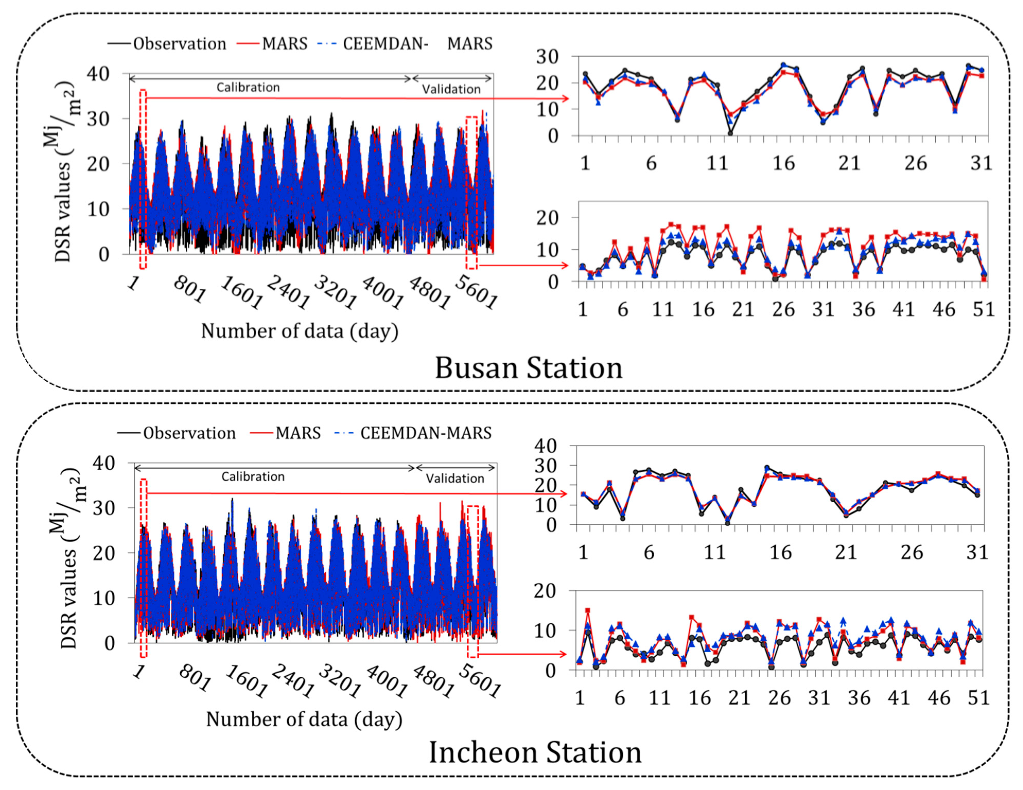
In addition, time series plots between forecasted and observed DSR values in the calibration and validation phases are shown in Figure 7. This figure explained that the observed and forecasted DSR values using CEEMDAN-MARS model showed better agreement than MARS model.

5.4. Standalone and Hybrid SaMARS Models

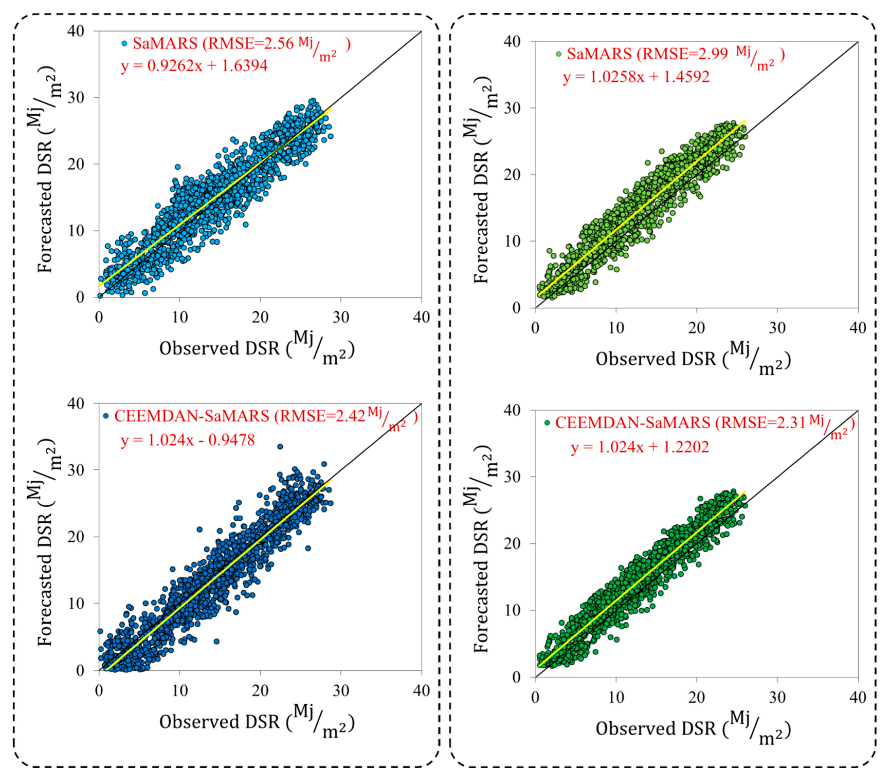
Table 5 explains that the CEEMDAN-SaMARS model outperforms the SaMARS model to forecast DSR in the calibration and validation phases at Busan. A combination of MARS model, CEEMDAN data pre-processing approach and CSA algorithm (RMSE = 2.427 MJ/m2, RRMSE = 0.181, MAE = 1.894 MJ/m2, NSE = 0.878, WI = 0.971, and LMI = 0.672) produces better results compared with the standalone SaMARS model (RMSE = 2.562 MJ/m2, RRMSE = 0.174, MAE = 2.092 MJ/m2, NSE = 0.864, WI = 0.964, and LMI = 0.638) for the validation phase at Busan.
At Incheon, comparison between SaMARS and CEEMDAN-SaMARS models suggested that the CEEMDAN-SaMARS model produces outstanding results (RMSE = 2.311 MJ/m2, RRMSE = 0.164, MAE = 1.931 MJ/m2, NSE = 0.883, WI = 0.967, and LMI = 0.659) compared with the SaMARS model (RMSE = 2.999 MJ/m2, RRMSE = 0.206, MAE = 2.455 MJ/m2, NSE = 0.769, WI = 0.948, and LMI = 0.537) for the validation phase at Incheon. Therefore, SaMARS model could not perform more efficiently than the CEEMDAN-SaMARS model for DSR forecasting at Incheon.
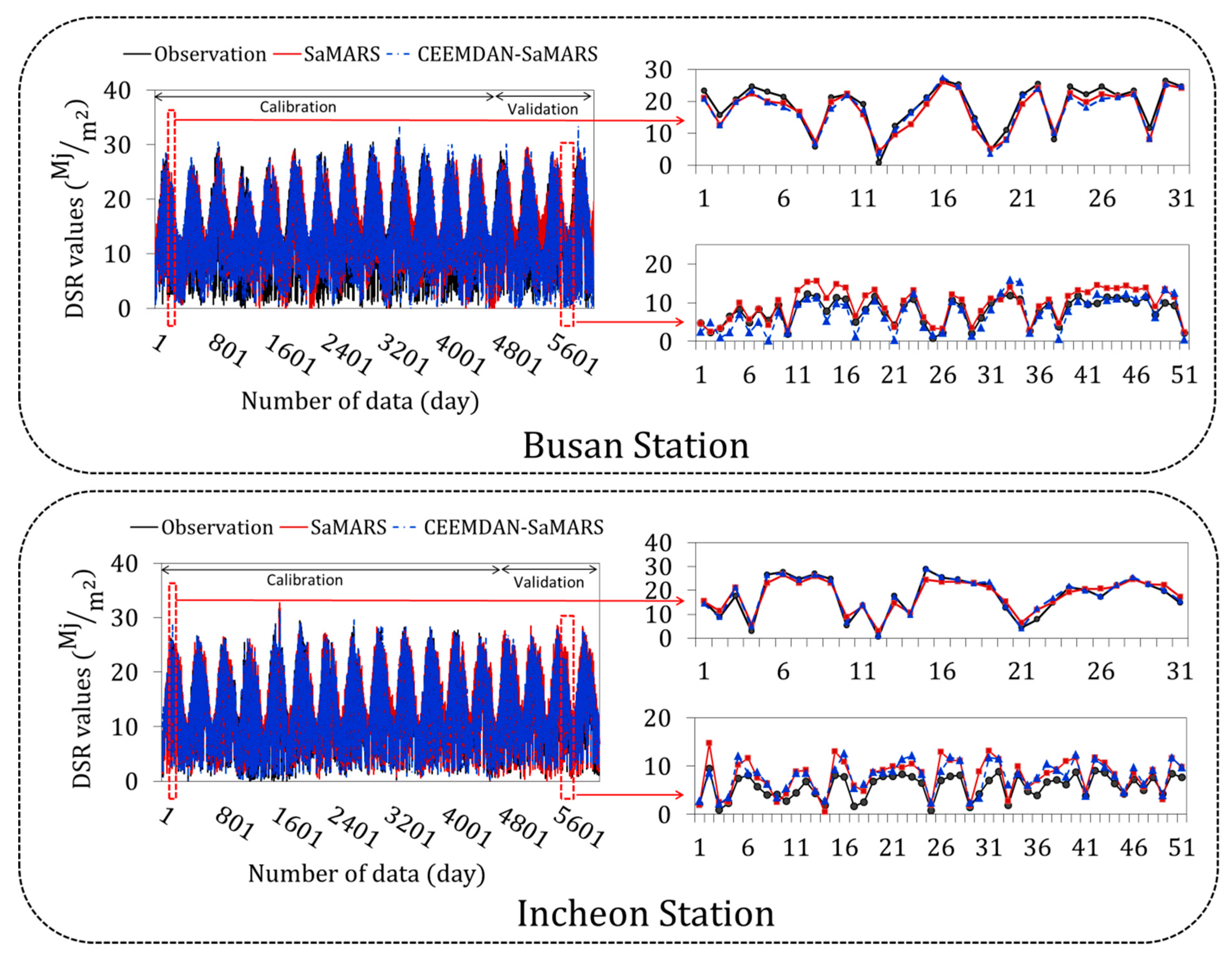
Scatterplots and time-series between observed and estimated DSR values at Busan are presented in Figure 8 and Figure 9, respectively. It can be found from Figure 8 and Figure 9 that the slopes of the forecasted DSR values using CEEMDAN-SaMARS are much close to the ideal value (y = x); this model performs better in comparison with SaMARS.
Likewise, at Incheon, Figure 8 and Figure 9 provide that the CEEMDAN-SaMARS model give fewer scattered estimates compared with SaMARS. In addition, the accuracy of the forecasted peak values from CEEMDAN-SaMARS is improved compared with SaMARS model. Therefore, the CEEMDAN-SaMARS model is found to be relatively more suitable for forecasting DSR peak values than SaMARS model in the validation phase in Incheon.

5.5. Comparison of Proposed Hybrid and Standalone Models

After the investigation of the standalone and hybrid models for DSR forecasting, the performance of the proposed models was generally compared to select the best for DSR forecasting of both stations. It can be seen from Table 3, Table 4 and Table 5 at Busan, that the values of forecasted DSR using CEEMDAN-MARS and CEEMDAN-SaMARS provided a reliable and efficient performances compared with CEEMDAN-GEP, GEP, MARS, and SaMARS. In a similar comparison at Incheon, the CEEMDAN-SaMARS produced the best results to forecast DSR compared with CEEMDAN-GEP, CEEMDAN-MARS, GEP, MARS, and SaMARS models. From the results at both stations, the conjunction of MARS model, CEEMDAN data pre-processing approach, and CSA algorithm produced the best results to forecast DSR. Therefore, it can be judged from this investigation that the application of CEEMDAN and CSA to standalone data-driven model can clearly enhance the model accuracy and efficiency.
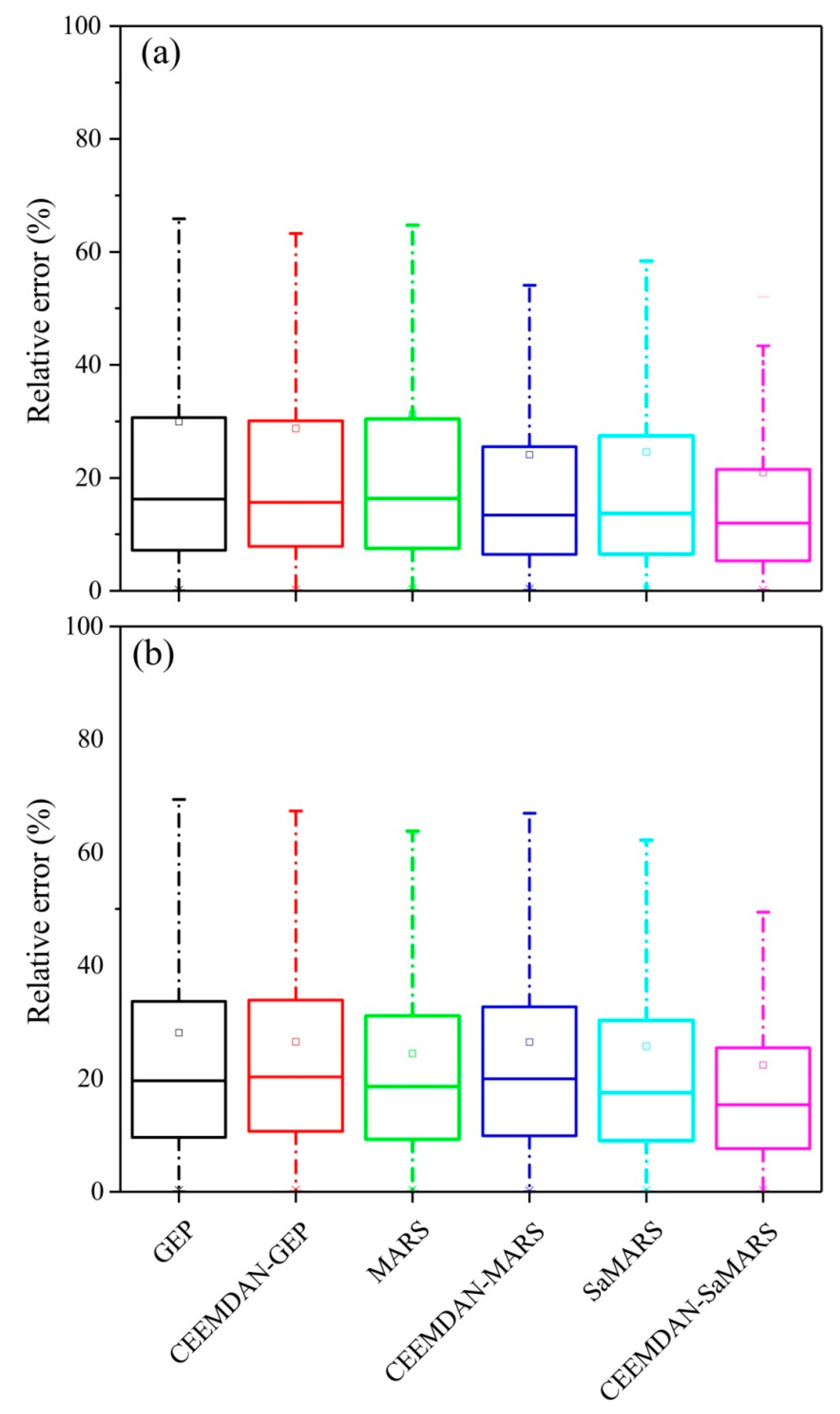
In addition, the forecasting accuracy of the proposed models is shown using box-plots diagrams (Figure 10). Box-plots can be expressed as the spread of observed and forecasted DSR data according to their quartiles. The whiskers indicate the outside variation of 25th (lower) and 75th (upper) percentiles [37]. Using the box-plots, the CEEMDAN-SaMARS model gave higher accuracy and ability to forecast DSR compared with the other models.
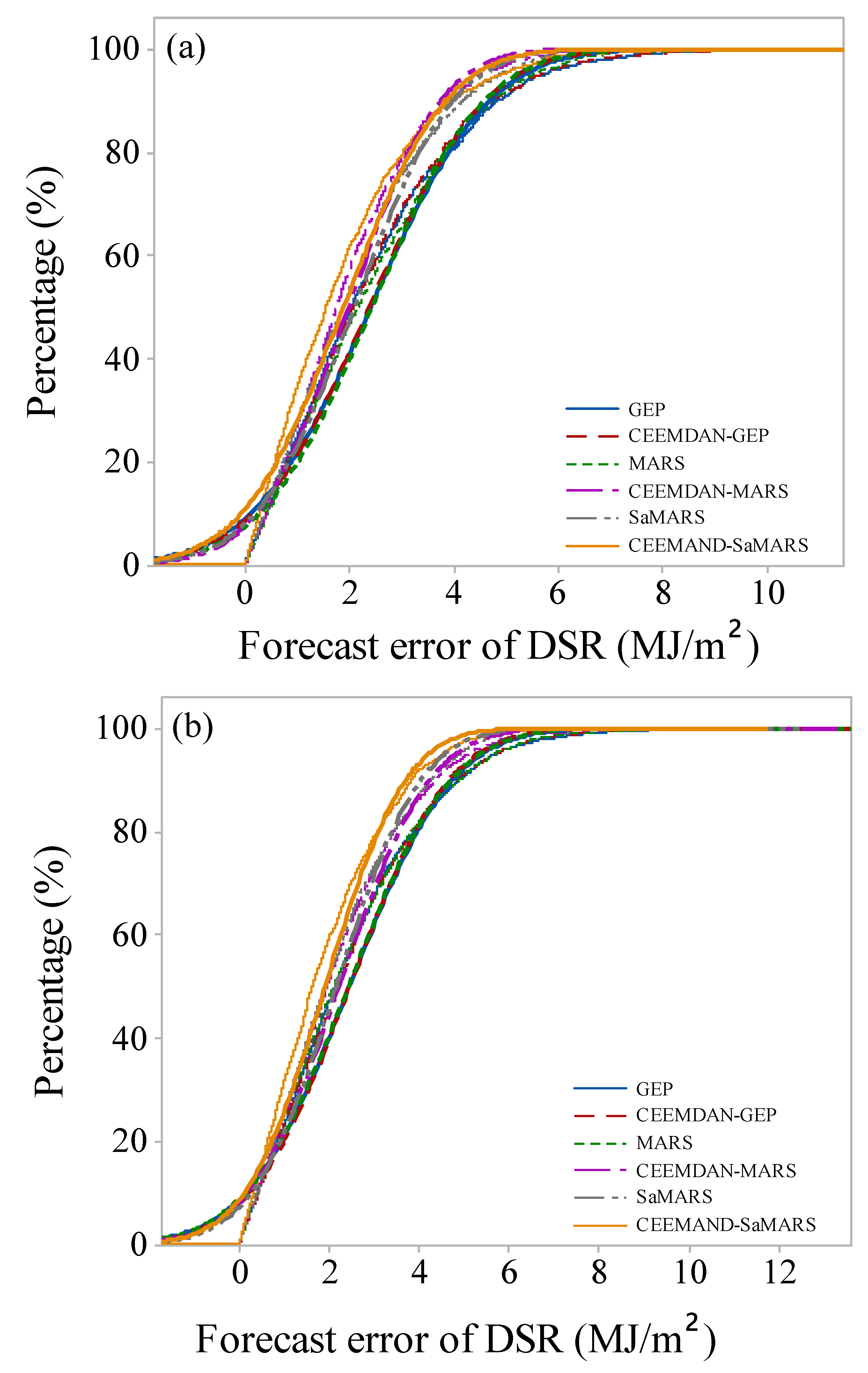
Furthermore, the percentage of absolute forecasted error value is represented using the empirical cumulative distribution function (ECDF) for the validation phase at both stations (Figure 11). Using the error percentage that indicates the minimum error (i.e., from 0 to ±4 MJ/m2), the CEEMDAN-SaMARS model gave the best performance compared with the other models for forecasting DSR values.
Overall, the results of this research indicate that the CEEMDAN-based GEP, MARS, and SaMARS models capture the non-linear and non-stationary dynamics of DSR time series datasets effectively and can provide optimal DSR forecasting. Although the GEP, MARS, SaMARS models could forecast DSR values, they were not efficient and accurate as CEEMDAN-GEP, CEEMDAN-MARS, and CEEMDAN-SaMARS models. Though, this study proposed and assessed the hybrid models (i.e., CEEMDAN-GEP, CEEMDAN-MARS, and CEEMDAN-SaMARS) for DSR forecasting, the identified limitations on DSR research must be taken into account for future studies.
This study explains that the GEP, MARS, and SaMARS models can improve the precision of DSR forecasting when the CEEMDAN method is integrated for decomposing data time-series into components. However, one of the main disadvantages of using the CEEMDAN data pre-processing approach would be classified as time-consumption. In addition, even if CSA algorithm shows excellent performance for determining three parameters of MARS, it has to develop and verify other meta-heuristic algorithms that help to identify the adequate parameters of MARS. The reason can be expressed that CSA algorithm requires a long time to find the parameter of MARS model. Although the outcomes are suitable for this research, other alternative methods have to be found, and investigated to solve this issue.

6. Conclusions and Future Research

Solar radiation is one of the most renewable and accessible energy sources, and plays a crucial role in global energy demand. Hence, accurate forecasting of DSR is one of the major problems for scientists, engineers, and decision makers. This study attempts to investigate the efficiency of GEP, MARS, and SaMARS models for DSR forecasting at Busan and Incheon stations, South Korea. To overcome the non-stationary and non-linear characteristics of time-series values, the CEEMDAN is utilized as the data pre-processing approach to decompose all input/output variables, which improves the accuracy of DSR forecasting.
Comparing the results of standalone models (e.g., GEP, MARS, and SaMARS) and hybrid models (e.g., CEEMDAN-GEP, CEEMDAN-MARS, and CEEMDAN-SaMARS) confirms the accuracy and efficiency of the proposed models. It is shown that the CEEMDAN data pre-processing approach has a significant influence on models’ accuracy and provides better results. At the Busan station, the forecasted DSR using CEEMDAN-GEP, CEEMDAN-MARS, and CEEMDAN-SaMARS models have a higher accuracy in term of NSE, 0.873, 0.879, and 0.878, compared to the standalone GEp, MARS, and SaMARS models. Furthermore, the results indicate that the CEEMDAN-SaMARS model is an effective tool and a promising method for DSR forecasting. The performance of the hybridized CEEMDAN-SaMARS model at both stations was the best, with RRMSE ≤ 18.1% at Busan and 19.3% at Incheon. In addition, this research reveals that the usage of a data pre-processing model (e.g., CEEMDAN) plays a main role in achieving an accurate forecast. Furthermore, future study is necessary to improve the model’s accuracy using feature selection methods to attain optimal input variables.
In spite of some limitations, this study can provide the basic information for future work, particularly the use of a hybrid model which can be integrated with a physically-based approach to create a DSR simulation model. Moreover, it is suggested that a two-phase decomposition is utilized to increase IMF1 estimating values which have a high frequency.

Author Contributions

M.R.-B. and F.B.-M. conceived and designed the study; S.K. and A.A. collected and pre-processed the data; M.R.-B. and N.M. implemented the models and performed the analyses; M.R.-B. and N.M. wrote the original draft of manuscript; N.W.K. and I.-M.C. analyzed the results; S.A. reviewed and edited the manuscript.

Funding

This research was funded by the Korea Institute of Civil Engineering and Building Technology, grant number 20190153-001.

Acknowledgments

This research was supported by a grant from a Strategic Research Project (Development of Hydrological Safety Assessment System for Hydraulic Structures) funded by the Korea Institute of Civil Engineering and Building Technology.

Conflicts of Interest

The authors declare no conflict of interest.

References

  1. Wu, Y.; Wang, J. A novel hybrid model based on artificial neural networks for solar radiation prediction. Renew. Energy 2016, 89, 268–284. [Google Scholar] [CrossRef]
  2. Demirhan, H.; Atilgan, Y.K. New horizontal global solar radiation estimation models for Turkey based on robust coplot supported genetic programming technique. Energy Convers. Manage. 2015, 106, 1013–1023. [Google Scholar] [CrossRef]
  3. Despotovic, M.; Nedic, V.; Despotovic, D.; Cvetanovic, S. Evaluation of empirical models for predicting monthly mean horizontal diffuse solar radiation. Renew. Sustain. Energy Rev. 2016, 56, 246–260. [Google Scholar] [CrossRef]
  4. Mohammadi, K.; Shamshirband, S.; Kamsin, A.; Lai, P.C.; Mansor, Z. Identifying the most significant input parameters for predicting global solar radiation using an ANFIS selection procedure. Renew. Sustain. Energy Rev. 2016, 63, 423–434. [Google Scholar] [CrossRef]
  5. Gairaa, K.; Khellaf, A.; Messlem, Y.; Chellali, F. Estimation of the daily global solar radiation based on Box–Jenkins and ANN models: A combined approach. Renew. Sustain. Energy Rev. 2016, 57, 238–249. [Google Scholar] [CrossRef]
  6. Shamshirband, S.; Mohammadi, K.; Chen, H.L.; Samy, G.N.; Petković, D.; Ma, C. Daily global solar radiation prediction from air temperatures using kernel extreme learning machine: A case study for Iran. J. Atmos. Sol.-Terr. Phy. 2015, 134, 109–117. [Google Scholar] [CrossRef]
  7. Gueymard, C.A. A review of validation methodologies and statistical performance indicators for modeled solar radiation data: Towards a better bankability of solar projects. Renew. Sustain. Energy Rev. 2014, 39, 1024–1034. [Google Scholar] [CrossRef]
  8. Rehman, S.; Mohandes, M. Artificial neural network estimation of global solar radiation using air temperature and relative humidity. Energy Policy 2008, 36, 571–576. [Google Scholar] [CrossRef] [Green Version]
  9. Olatomiwa, L.; Mekhilef, S.; Shamshirband, S.; Petković, D. Adaptive neuro-fuzzy approach for solar radiation prediction in Nigeria. Renew. Sustain. Energy Rev. 2015, 51, 1784–1791. [Google Scholar] [CrossRef]
  10. Zeng, J.; Qiao, W. Short-term solar power prediction using a support vector machine. Renew. Energy 2013, 52, 118–127. [Google Scholar] [CrossRef]
  11. Wang, L.; Kisi, O.; Zounemat-Kermani, M.; Zhu, Z.; Gong, W.; Niu, Z.; Liu, Z. Prediction of solar radiation in China using different adaptive neuro-fuzzy methods and M5 model tree. Int. J. Climatol. 2017, 37, 1141–1155. [Google Scholar] [CrossRef]
  12. Kim, S.; Seo, Y.; Rezaie-Balf, M.; Kisi, O.; Ghorbani, M.A.; Singh, V.P. Evaluation of daily solar radiation flux using soft computing approaches based on different meteorological information: peninsula vs continent. Theor. Appl. Climatol. 2018, 1–20. [Google Scholar] [CrossRef]
  13. Landeras, G.; López, J.J.; Kisi, O.; & Shiri, J. Comparison of Gene Expression Programming with neuro-fuzzy and neural network computing techniques in estimating daily incoming solar radiation in the Basque Country (Northern Spain). Energy Convers. Manag. 2012, 62, 1–13. [Google Scholar] [CrossRef]
  14. Yadav, A.K.; Chandel, S.S. Solar radiation prediction using Artificial Neural Network techniques: A review. Renew. Sustain. Energy Rev. 2014, 33, 772–781. [Google Scholar] [CrossRef]
  15. Sozen, A.; Arcakliogblu, E.; Ozalp, M. Estimation of solar potential in Turkey by artificial neural networks using meteorological and geographical data. Energy Convers. Manag. 2004, 45, 3033–3052. [Google Scholar] [CrossRef]
  16. Dorvlo, A.S.; Jervase, J.A.; Al-Lawati, A. Solar radiation estimation using artificial neural networks. Appl. Energy 2002, 71, 307–319. [Google Scholar] [CrossRef]
  17. Alsina, E.F.; Bortolini, M.; Gamberi, M.; Regattieri, A. Artificial neural network optimisation for monthly average daily global solar radiation prediction. Energy Convers. Manag. 2016, 120, 320–329. [Google Scholar] [CrossRef]
  18. Lou, S.; Li, D.H.; Lam, J.C.; Chan, W.H. Prediction of diffuse solar irradiance using machine learning and multivariable regression. Appl. Energy 2016, 181, 367–374. [Google Scholar] [CrossRef]
  19. Mohammadi, K.; Shamshirband, S.; Tong, C.W.; Arif, M.; Petković, D.; Ch, S. A new hybrid support vector machine–wavelet transform approach for estimation of horizontal global solar radiation. Energy Convers. Manag. 2015, 92, 162–171. [Google Scholar] [CrossRef]
  20. Antonanzas, J.; Urraca, R.; Martinez-de-Pison, F.J.; Antonanzas-Torres, F. Solar irradiation mapping with exogenous data from support vector regression machines estimations. Energy Convers. Manag. 2015, 100, 380–390. [Google Scholar] [CrossRef]
  21. Monteiro, R.V.; Guimarães, G.C.; Moura, F.A.; Albertini, M.R.; Albertini, M.K. Estimating photovoltaic power generation: performance analysis of artificial neural networks, Support Vector Machine and Kalman filter. Electr. Power Syst. Res. 2017, 143, 643–656. [Google Scholar] [CrossRef]
  22. Chen, J.L.; Liu, H.B.; Wu, W.; Xie, D.T. Estimation of monthly solar radiation from measured temperatures using support vector machines – a case study. Renew. Energy 2011, 36, 413–420. [Google Scholar] [CrossRef]
  23. Salcedo-Sanz, S.; Deo, R.C.; Cornejo-Bueno, L.; Camacho-Gómez, C.; Ghimire, S. An efficient neuro-evolutionary hybrid modelling mechanism for the estimation of daily global solar radiation in the Sunshine State of Australia. Appl. Energy 2018, 209, 79–94. [Google Scholar] [CrossRef]
  24. Hu, T.; Wu, F.; Zhang, X. Rainfall–runoff modeling using principal component analysis and neural network. Hydrol. Res. 2007, 38, 235–248. [Google Scholar] [CrossRef]
  25. Ravikumar, P.; Somashekar, R.K. Principal component analysis and hydrochemical facies characterization to evaluate groundwater quality in Varahi river basin, Karnataka state, India. Appl. Water Sci. 2017, 7, 745–755. [Google Scholar] [CrossRef]
  26. Sang, Y.F.; Wang, Z.; Liu, C. Discrete wavelet-based trend identification in hydrologic time series. Hydrol. Process. 2013, 27, 2021–2031. [Google Scholar] [CrossRef]
  27. Rezaie-Balf, M.; Naganna, S.R.; Ghaemi, A.; Deka, P.C. Wavelet coupled MARS and M5 Model Tree approaches for groundwater level forecasting. J. Hydrol. 2017, 553, 356–373. [Google Scholar] [CrossRef]
  28. Deo, R.C.; Wen, X.; Qi, F. A wavelet-coupled support vector machine model for forecasting global incident solar radiation using limited meteorological dataset. Appl. Energy 2016, 168, 568–593. [Google Scholar] [CrossRef]
  29. Yuan, X.; Tan, Q.; Lei, X.; Yuan, Y.; Wu, X. Wind power prediction using hybrid autoregressive fractionally integrated moving average and least square support vector machine. Energy 2017, 129, 122–137. [Google Scholar] [CrossRef]
  30. Zakhrouf, M.; Bouchelkia, H.; Stamboul, M.; Kim, S.; Heddam, S. Time series forecasting of river flow using an integrated approach of wavelet multi-resolution analysis and evolutionary data-driven models. A case study: Sebaou River (Algeria). Phys. Geogr. 2018, 39, 506–522. [Google Scholar] [CrossRef]
  31. Benedetto, F.; Giunta, G.; Mastroeni, L. A maximum entropy method to assess the predictability of financial and commodity prices. Digit. Signal. Process. 2015, 46, 19–31. [Google Scholar] [CrossRef]
  32. Baykasoğlu, A.; Güllü, H.; Çanakçı, H.; Özbakır, L. Prediction of compressive and tensile strength of limestone via genetic programming. Expert Syst. Appl. 2008, 35, 111–123. [Google Scholar] [CrossRef]
  33. Liu, H.; Mi, X.; Li, Y. Smart multi-step deep learning model for wind speed forecasting based on variational mode decomposition, singular spectrum analysis, LSTM network and ELM. Energy Convers. Manag. 2018, 159, 54–64. [Google Scholar] [CrossRef]
  34. Rezaie-Balf, M.; Kisi, O.; Chua, L.H. Application of ensemble empirical mode decomposition based on machine learning methodologies in forecasting monthly pan evaporation. Hydrol. Res. 2018. [Google Scholar] [CrossRef]
  35. Al-Musaylh, M.S.; Deo, R.C.; Li, Y.; Adamowski, J.F. Two-phase particle swarm optimized-support vector regression hybrid model integrated with improved empirical mode decomposition with adaptive noise for multiple-horizon electricity demand forecasting. Appl. Energy 2018, 217, 422–439. [Google Scholar] [CrossRef]
  36. Zhang, W.; Qu, Z.; Zhang, K.; Mao, W.; Ma, Y.; Fan, X. A combined model based on CEEMDAN and modified flower pollination algorithm for wind speed forecasting. Energy Convers. Manag. 2017, 136, 439–451. [Google Scholar] [CrossRef]
  37. Prasad, R.; Deo, R.C.; Li, Y.; Maraseni, T. Ensemble committee-based data intelligent approach for generating soil moisture forecasts with multivariate hydro-meteorological predictors. Soil. Till. Res. 2018, 181, 63–81. [Google Scholar] [CrossRef]
  38. Wen, X.; Feng, Q.; Deo, R.C.; Wu, M.; Yin, Z.; Yang, L.; Singh, V.P. Two-phase extreme learning machines integrated with complete ensemble empirical mode decomposition with adaptive noise for multi-scale runoff prediction. J. Hydrol. 2019, 570, 167–184. [Google Scholar] [CrossRef]
  39. Bailek, N.; Bouchouicha, K.; Al-Mostafa, Z.; El-Shimy, M.; Aoun, N.; Slimani, A.; Al-Shehri, S. A new empirical model for forecasting the diffuse solar radiation over Sahara in the Algerian Big South. Renew. Energy 2018, 117, 530–537. [Google Scholar] [CrossRef]
  40. Wu, Z.; Huang, N.E. Ensemble empirical mode decomposition: A noise-assisted data analysis method. Adv. Adapt. Data Anal. 2009, 1, 1–41. [Google Scholar] [CrossRef]
  41. Huang, N.E.; Shen, Z.; Long, S.R.; Wu, M.C.; Shih, H.H.; Zheng, Q.; Yen, N.C.; Chi, C.T.; Liu, H.H. The empirical mode decomposition and the hilbert spectrum for nonlinear and non-stationary time series analysis. Proc. Math. Phys. Eng. Sci. 1998, 454, 903–995. [Google Scholar] [CrossRef]
  42. Lei, Y.; He, Z.; Zi, Y. Application of the EEMD method to rotor fault diagnosis of rotating machinery. Mech. Syst. Signal. Pr. 2009, 23, 1327–1338. [Google Scholar] [CrossRef]
  43. Torres, M.E.; Colominas, M.A.; Schlotthauer, G.; Flandrin, P. A complete ensemble empirical mode decomposition with adaptive noise. In Proceedings of the 2011 IEEE International Conference on Acoustics, Speech and Signal Processing (ICASSP), Prague, Czech Republic, 22–27 May 2011; pp. 4144–4147. [Google Scholar]
  44. Ferreira, C. Gene expression programming in problem solving. In Soft Computing and Industry; Springer: London, UK, 2002; pp. 635–653. [Google Scholar]
  45. Gholampour, A.; Gandomi, A.H.; Ozbakkaloglu, T. New formulations for mechanical properties of recycled aggregate concrete using gene expression programming. Constr. Build. Mat. 2017, 130, 122–145. [Google Scholar] [CrossRef]
  46. Ferreira, C. Gene expression programming and the evolution of computer programs. In Recent Developments in Biologically Inspired Computing; Idea Group Publishing: Hershey, PA, USA, 2005; pp. 82–103. [Google Scholar]
  47. Hossein Alavi, A.; Hossein Gandomi, A. A robust data mining approach for formulation of geotechnical engineering systems. Eng. Comput. 2011, 28, 242–274. [Google Scholar] [CrossRef]
  48. Friedman, J. Multivariate Adaptive Regression Splines. Ann. Stat. 1991, 19, 1–67. [Google Scholar] [CrossRef] [Green Version]
  49. Kisi, O. Pan evaporation modeling using least square support vector machine, multivariate adaptive regression splines and M5 model tree. J. Hydrol. 2015, 528, 312–320. [Google Scholar] [CrossRef]
  50. Rezaie-Balf, M. Multivariate Adaptive Regression Splines Model for Prediction of Local Scour Depth Downstream of an Apron Under 2D Horizontal Jets. Iran. J. Sci. Tech. Trans. Civil Eng. 2018, 1–13. [Google Scholar] [CrossRef]
  51. Zhang, W.G.; Goh, A.T.C. Multivariate adaptive regression splines for analysis of geotechnical engineering systems. Comput. Geotech. 2013, 48, 82–95. [Google Scholar] [CrossRef]
  52. Conoscenti, C.; Ciaccio, M.; Caraballo-Arias, N.A.; Gómez-Gutiérrez, Á.; Rotigliano, E.; Agnesi, V. Assessment of susceptibility to earth-flow landslide using logistic regression and multivariate adaptive regression splines: A case of the Belice River basin (western Sicily, Italy). Geomorphology 2015, 242, 49–64. [Google Scholar] [CrossRef]
  53. Zhang, W.; Goh, A.T. Multivariate adaptive regression splines and neural network models for prediction of pile drivability. Geosci. Front. 2016, 7, 45–52. [Google Scholar] [CrossRef] [Green Version]
  54. Askarzadeh, A. A novel metaheuristic method for solving constrained engineering optimization problems: crow search algorithm. Comput. Struct. 2016, 169, 1–12. [Google Scholar] [CrossRef]
  55. Gupta, D.; Rodrigues, J.J.; Sundaram, S.; Khanna, A.; Korotaev, V.; de Albuquerque, V.H.C. Usability feature extraction using modified crow search algorithm: A novel approach. Neural Comput. Appl. 2018, 1–11. [Google Scholar] [CrossRef]
  56. Nash, J.E.; Sutcliffe, J.V. River flow forecasting through conceptual models, Part 1—A discussion of principles. J. Hydrol. 1970, 10, 282–290. [Google Scholar] [CrossRef]
  57. Willmott, C.J.; Robeson, S.M.; Matsuura, K. A refined index of model performance. Int. J. Climatol. 2012, 32, 2088–2094. [Google Scholar] [CrossRef]
  58. Legates, D.R.; McCabe, G.J. Evaluating the use of “goodness-of-fit” measures in hydrologic and hydroclimatic model validation. Water Resour. Res. 1999, 35, 233–241. [Google Scholar] [CrossRef]
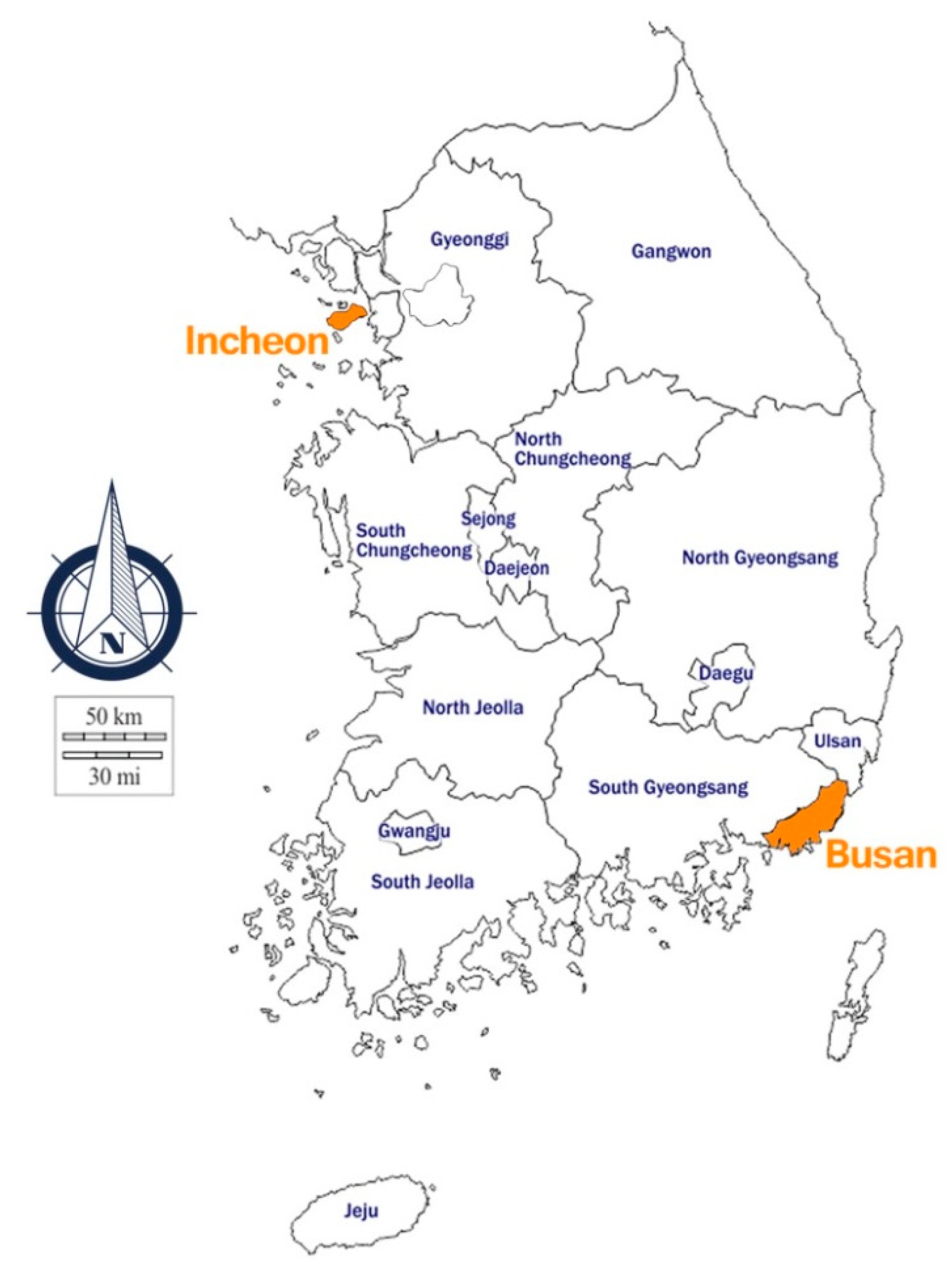
Figure 1. Map of study area.
Energies 12 01416 g001
Figure 2. Intrinsic mode functions (IMFs) and residual constructed using CEEMDAN for daily solar radiation at Busan station (calibration phase).
Energies 12 01416 g002
Figure 3. The main procedures of proposed standalone and hybrid models.
Energies 12 01416 g003
Figure 4. Scatterplots of observed and forecasted DSR using the GEP and CEEMDAN-GEP models in validation phase at Busan (blue color) and Incheon (Green color) stations.
Energies 12 01416 g004
Figure 5. Time-series plots between observed and forecasted DSR for GEP and CEEMDAN-GEP models for calibration and validation phases at Busan and Incheon stations.
Energies 12 01416 g005
Figure 6. Scatterplots of observed and forecasted DSR using the MARS and CEEMDAN-MARS models in the validation phase at Busan (blue color) and Incheon (Green color) stations.
Energies 12 01416 g006
Figure 7. Time-series plots between observed and forecasted DSR for MARS and CEEMDAN-MARS models for the calibration and validation phases at Busan and Incheon.
Energies 12 01416 g007
Figure 8. Scatterplots of observed and forecasted DSR using the SaMARS and CEEMDAN-SaMARS models in the validation phase at Busan (blue color) and Incheon (Green color) stations.
Energies 12 01416 g008
Figure 9. Time-series plots between observed and forecasted DSR for SaMARS and CEEMDAN-SaMARS models for the calibration and validation phases at Busan and Incheon stations.
Energies 12 01416 g009
Figure 10. Box-plots of relative error of forecasted values of DSR (MJ/m2) using the standalone and hybrid models at (a) Busan (b) Incheon stations in the validation phase.
Energies 12 01416 g010
Figure 11. Empirical cumulative distribution function of the absolute forecasted error (MJ/m2) using the standalone and hybrid models at (a) Busan (b) Incheon stations in the validation phase.
Energies 12 01416 g011
Table 1. Descriptive statistics of solar radiation data for the Busan and Incheon stations located in South Korea.
Statistical ParameterMeteorological Variable
TA (°C)RH (%)VP (hPa)SLP (hPa)PE (cm)SD (hr)DSR (MJ/m2)
Busan station (calibration data, 2000–2012)
Minimum−7.211.30.8992.20.20.00.0
Mean14.862.212.91015.53.16.114.1
Maximum30.199.037.21036.28.813.131.3
Standard deviation8.218.88.47.11.53.97.0
Coefficient of variation 66.5354.770.551.12.214.949.4
Skewness index−0.3−0.20.5−0.10.5−0.30.1
Busan station (validation data, 2013–2016)
Minimum−7.617.61.1992.70.00.00.2
Mean15.464.113.41015.83.47.114.0
Maximum31.799.933.11034.411.513.128.7
Standard deviation8.117.88.37.41.74.17.0
Coefficient of variation 66.0318.668.655.32.917.048.3
Skewness index−0.3−0.20.4−0.10.5−0.60.1
Incheon station (calibration data, 2000–2012)
Minimum−14.625.00.9990.80.00.00.0
Mean12.667.312.21016.13.06.012.9
Maximum31.1100.034.11039.012.013.732.1
Standard deviation9.815.08.38.11.83.96.9
Coefficient of variation 97.0224.868.365.43.315.547.1
Skewness index−0.3−0.10.60.00.7−0.20.2
Incheon station (validation data, 2013–2016)
Minimum−13.131.01.3991.20.00.00.5
Mean12.877.314.21016.43.47.112.5
Maximum30.899.038.31037.610.113.926.0
Standard deviation10.114.89.68.32.03.96.2
Coefficient of variation 101.9217.692.269.34.115.539.0
Skewness index−0.3−0.40.60.00.5−0.50.2
TA, RH, VP, SLP, PE, SD and DSR denote the air temperature, relative humidity, vapor pressure, sea-level pressure, pan evaporation, sunshine duration, and daily solar radiation, respectively.
Table 2. Design parameters of GEP and MARS models for calibration stage at Busan and Incheon stations.
ModelDesign Parameter
GEPChromosomesGene sizeHead sizeLinking functionMutation rateCrossover rateOne and two- point recombination rateIS and RIS transposition rate
3038Addition0.010.80.30.1
MARSMax functionGCVSelf- interactionsMax interactionsThresholdPrune--
25–400, 2–4No2–41.0 × 10⁻⁴Yes--
Table 3. Statistical performance of standalone and hybrid GEP models at Busan and Incheon stations.
Model (Station)RMSE (MJ/m2)RRMSEMAE (MJ/m2)NSEWILMI
Calibration phase
GEP (Busan)2.3950.1691.9040.8830.9680.674
CEEMDAN-GEP (Busan)2.1730.1411.7270.9050.9780.712
GEP (Incheon)2.4080.1931.8720.8770.9680.675
CEEMDAN-GEP (Incheon)2.1990.1711.6930.8970.9720.706
Validation phase
GEP (Busan)2.9920.1892.4020.8140.9550.585
CEEMDAN-GEP (Busan)2.5140.1711.9950.8730.9740.654
GEP (Incheon)3.0860.2112.5010.7550.9440.528
CEEMDAN-GEP (Incheon)2.8620.1922.3240.7890.9520.564
Table 4. Statistical performance of standalone and hybrid MARS models at Busan and Incheon stations.
Model (Station)RMSE (MJ/m2)RRMSEMAE (MJ/m2)NSEWILMI
Calibration phase
MARS (Busan)2.7420.1942.1830.8470.9570.626
CEEMDAN-MARS (Busan)2.2050.1561.7620.9010.9730.698
MARS (Incheon)2.3460.18241.8320.8830.9680.681
CEEMDAN-MARS (Incheon)1.9010.1461.5060.9230.9790.738
Validation phase
MARS (Busan)2.9510.2072.4370.8190.9510.581
CEEMDAN-MARS (Busan)2.4120.1661.9830.8790.9690.667
MARS (Incheon)3.0660.2142.4210.7580.9480.544
CEEMDAN-MARS (Incheon)2.6590.1852.2210.8180.9570.582
Table 5. Statistical performance of standalone and hybrid SaMARS models at Busan and Incheon stations.
Model (Station)RMSE (MJ/m2)RRMSEMAE (MJ/m2)NSEWILMI
Calibration phase
SaMARS (Busan)2.3860.1691.8870.8840.9680.677
CEEMDAN-SaMARS (Busan)1.8280.1291.4310.9320.9820.776
SaMARS (Incheon)2.1980.1710.17140.8970.9720.702
CEEMDAN-SaMARS (Incheon)1.0010.0770.6150.9780.9940.893
Validation phase
SaMARS (Busan)2.5620.1742.0920.8640.9640.638
CEEMDAN-SaMARS (Busan)2.4270.1811.8940.8780.9710.672
SaMARS (Incheon)2.9990.2062.4550.7690.9480.537
CEEMDAN-SaMARS (Incheon)2.3110.1641.9310.8830.9670.659