Shales Leaching Modelling for Prediction of Flowback Fluid Composition


Abstract
:1. Introduction
2. Materials and Methods
2.1. Shale Sample Acquisition
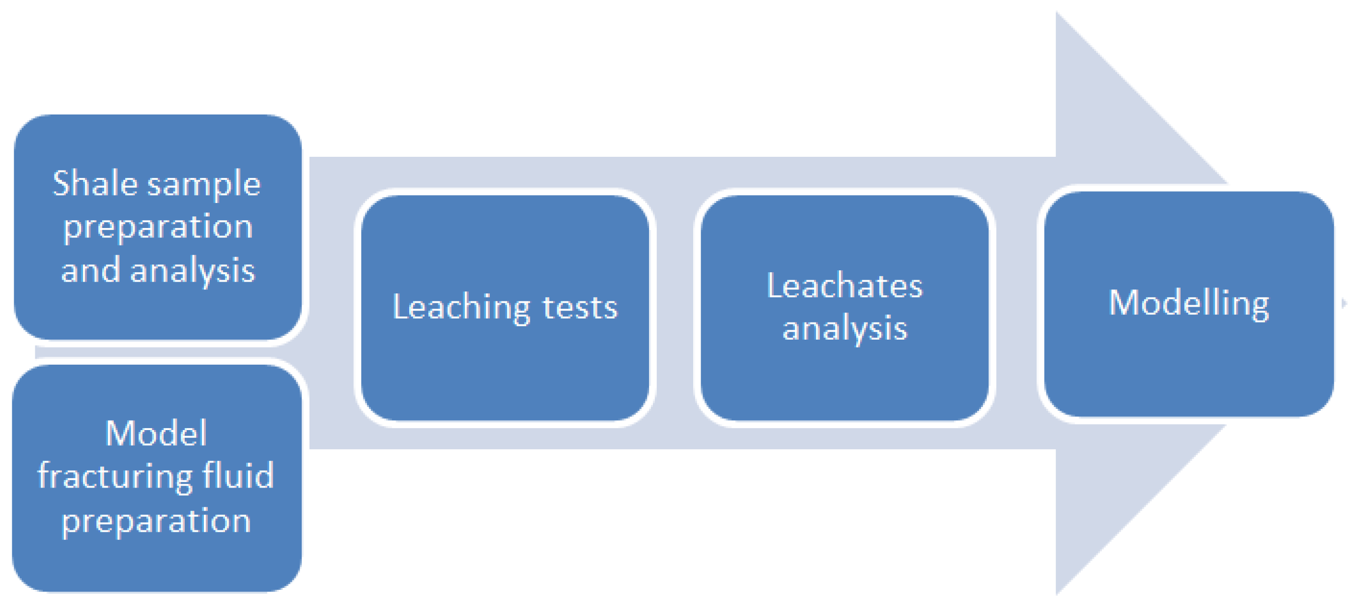
2.2. Shale Sample Preparation
2.3. Shale Samples Analysis
2.4. Preparation of Model Fracturing Fluids
2.5. Leaching Tests
3. Results and Discussion
4. Conclusions
Author Contributions
Funding
Conflicts of Interest
Appendix A

| No. Shale Sample | Mineral (%) | |||||||||||||||
|---|---|---|---|---|---|---|---|---|---|---|---|---|---|---|---|---|
| Quarz | Alb | Micr | Ort | Calc | Dol | Pir | Bar | Chl | Ill | Mon | Kao | Mus | Bio | Par | Gla | |
| A1 | 15.89 | 2.93 | 1.58 | 1.10 | 9.38 | 2.56 | 6.70 | 2.43 | 4.75 | 1.10 | 0.00 | 9.38 | 38.29 | 0.36 | 2.56 | 0.98 |
| A2 | 21.58 | 1.83 | 1.10 | 0.74 | 2.93 | 0.74 | 0.00 | 0.08 | 7.19 | 0.74 | 0.00 | 2.81 | 57.48 | 1.58 | 0.61 | 0.61 |
| A3 | 12.74 | 2.07 | 2.68 | 0.61 | 28.67 | 8.53 | 0.00 | 0.12 | 3.77 | 0.48 | 10.73 | 5.85 | 18.64 | 2.93 | 1.83 | 0.36 |
| A4 | 19.58 | 3.10 | 5.08 | 0.37 | 21.52 | 3.97 | 0.00 | 0.25 | 7.81 | 8.80 | 0.00 | 1.86 | 2.61 | 22.81 | 1.11 | 1.11 |
| A5 | 23.73 | 0.98 | 0.86 | 0.37 | 22.81 | 4.80 | 0.00 | 0.12 | 9.34 | 2.83 | 0.12 | 11.55 | 19.17 | 0.62 | 0.86 | 1.85 |
| A6 | 22.57 | 3.44 | 2.59 | 0.74 | 13.05 | 30.67 | 1.73 | 0.12 | 4.06 | 1.73 | 0.00 | 0.37 | 13.29 | 0.24 | 3.32 | 2.09 |
| A7 | 13.60 | 2.70 | 3.19 | 0.12 | 12.86 | 33.97 | 0.12 | 0.12 | 5.03 | 3.19 | 0.24 | 0.36 | 17.27 | 4.53 | 0.50 | 2.20 |
| A8 | 25.66 | 4.16 | 2.08 | 0.62 | 8.44 | 16.50 | 0.00 | 0.12 | 4.88 | 0.74 | 0.00 | 0.36 | 33.76 | 0.48 | 1.72 | 0.48 |
| A9 | 34.97 | 6.67 | 3.52 | 1.00 | 9.17 | 11.19 | 0.76 | 0.12 | 5.04 | 2.13 | 0.00 | 2.13 | 5.53 | 3.77 | 1.51 | 12.47 |
| A10 | 21.81 | 2.18 | 1.09 | 0.48 | 9.82 | 12.13 | 0.12 | 0.00 | 7.52 | 0.48 | 0.00 | 1.21 | 41.45 | 0.36 | 0.97 | 0.36 |
References
- Dayal, A.M. Shale. In Shale Gas: Exploration and Environmental and Economic Impacts; Elsevier Science: Amsterdam, Holand, 2017; ISBN 9780128095355. [Google Scholar]
- Singh, K.; Holditch, S.A.; Ayers, W.B. Basin Analog Investigations Answer Characterization Challenges of Unconventional Gas Potential in Frontier Basins. J. Energy Resour. Technol. 2008, 130. [Google Scholar] [CrossRef]
- Chopra, S.; Solutions, A.S.; Kumar, R.; Marfurt, K.J. Current Workflows for Shale Gas Reservoir Characterization. In Proceedings of the Unconventional Resources Technology Conference, Denver, CO, USA, 12–14 August 2013. [Google Scholar] [CrossRef]
- Chermak, J.A.; Schreiber, M.E. Mineralogy and trace element geochemistry of gas shales in the United States: Environmental implications. Int. J. Coal Geol. 2014, 126, 32–44. [Google Scholar] [CrossRef]
- Liu, J.; Yao, Y.; Elsworth, D.; Liu, D.; Cai, Y.; Dong, L. Vertical heterogeneity of the shale reservoir in the lower silurian longmaxi formation: Analogy between the southeastern and Northeastern Sichuan Basin, SW China. Minerals 2017, 7, 151. [Google Scholar] [CrossRef]
- Barnhoorn, A.; Houben, M.E.; Lie-A-Fat, J.; Ravestein, T.; Drury, M. Variations in petrophysical properties of shales along a stratigraphic section in the Whitby mudstone (UK). In Proceedings of the EGU General Assembly 2015, Vienna, Austria, 12–17 April 2015. [Google Scholar]
- Chen, L.; Lu, Y.; Jiang, S.; Li, J.; Guo, T.; Luo, C. Heterogeneity of the lower silurian longmaxi marine shale in the southeast sichuan basin of China. Mar. Pet. Geol. 2015, 65, 232–246. [Google Scholar] [CrossRef]
- Rogala, A.; Krzysiek, J.; Bernaciak, M.; Hupka, J. Non-aqueous fracturing technologies for shale gas recovery. Physicochem. Probl. Miner. Process. 2013, 49, 313–322. [Google Scholar]
- Rogala, A.; Ksiezniak, K.; Krzysiek, J.; Hupka, J. Carbon dioxide sequestration during shale gas recovery. Physicochem. Probl. Miner. Process. 2014, 50, 681–692. [Google Scholar]
- Howard, G.C.; FAST, C.R. Hydraulic Fracturing; Henry L. Doherty Memorial Fund of AIME: New York, NY, USA, 1970; Volume 2, ISBN 0895202018. [Google Scholar]
- Tao, H.; Zhang, L.; Liu, Q.; Deng, Q.; Luo, M.; Zhao, Y. An Analytical Flow Model for Heterogeneous Multi-Fractured Systems in Shale Gas Reservoirs. Energies 2018, 11, 3422. [Google Scholar] [CrossRef]
- Economides, M.J.; Martin, T. Modern Fracturing—Enhancing Natural Gas Production; Energy Tribune Publishing: Houston, TX, USA, 2007; 509p. [Google Scholar]
- Gandossi, L. An Overview of Hydraulic Fracturing and Other Formation Stimulation Technologies for Shale Gas Production; Joint Research Centre: Mercier, Luxembourg, 2015; ISBN 9789279347290. [Google Scholar]
- Mader, D. Hydraulic Proppant Fracturing and Gravel Packing; Elsevier Science: Amsterdam, Holand, 1989; ISBN 9780444873521. [Google Scholar]
- Ksiezniak, K.; Rogala, A.; Hupka, J. Wettability of shale rock as an indicator of fracturing fluid composition. Physicochem. Probl. Miner. Process. 2015, 51, 315–323. [Google Scholar]
- Albrycht, I.; Boy, K.; Jankowski, J.M. Gaz Niekonwencjonalny—Szansa dla Polski i Europy? Analiza i Rekomendacje; Instytut Kościuszki: Kraków, Poland, 2011; ISBN 9788393109340. [Google Scholar]
- Arthur, J.D.; Bohm, B.K.; Cornue, D. Environmental Considerations of Modern Shale Gas Development. In Proceedings of the SPE Annual Technical Conference and Exhibition, San Antonio, TX, USA, 9–11 October 2009. [Google Scholar]
- Hayes, T.; Severin, B.F. Barnett and Appalachian Shale Water Management and Reuse Technologies; Project Report by Gas Technology Institute Research Partners toSecure Energy for America; Publications Office of the European Union: Mercier, Luxembourg, 2012; pp. 1–10. [Google Scholar]
- Boschee, P. Produced and Flowback Water Recycling and Reuse: Economics, Limitations, and Technology. Oil Gas Facil. 2014, 3, 16–21. [Google Scholar] [CrossRef]
- Abualfaraj, N.; Gurian, P.L.; Olson, M.S. Assessing residential exposure risk from spills of flowback water from Marcellus shale hydraulic fracturing activity. Int. J. Environ. Res. Public Health 2018, 11, 15. [Google Scholar] [CrossRef]
- Zhou, J.; Zhang, L.; Braun, A.; Han, Z. Investigation of processes of interaction between hydraulic and natural fractures by PFC modeling comparing against laboratory experiments and analytical models. Energies 2017, 10, 1001. [Google Scholar] [CrossRef]
- Clarkson, C.R.; Williams-Kovacs, J. Modeling Two-Phase Flowback of Multifractured Horizontal Wells Completed in Shale. SPE J. 2013, 18. [Google Scholar] [CrossRef]
- Williams-Kovacs, J.D.; Clarkson, C.R. A modified approach for modeling two-phase flowback from multi-fractured horizontal shale gas wells. J. Nat. Gas Sci. Eng. 2016, 30, 127–147. [Google Scholar] [CrossRef]
- Clarkson, C.R.; Haghshenas, B.; Ghanizadeh, A.; Qanbari, F.; Williams-Kovacs, J.D.; Riazi, N.; Debuhr, C.; Deglint, H.J. Nanopores to megafractures: Current challenges and methods for shale gas reservoir and hydraulic fracture characterization. J. Nat. Gas Sci. Eng. 2016. [Google Scholar] [CrossRef]
- Jia, P.; Cheng, L.; Clarkson, C.R.; Huang, S.; Wu, Y.; Williams-Kovacs, J.D. A novel method for interpreting water data during flowback and early-time production of multi-fractured horizontal wells in shale reservoirs. Int. J. Coal Geol. 2018, 200, 186–196. [Google Scholar] [CrossRef]
- Cao, P.; Liu, J.; Leong, Y.K. A multiscale-multiphase simulation model for the evaluation of shale gas recovery coupled the effect of water flowback. Fuel 2017, 199, 191–205. [Google Scholar] [CrossRef]
- Bai, B.; Elgmati, M.; Zhang, H.; Wei, M. Rock characterization of Fayetteville shale gas plays. Fuel 2013, 105, 642–652. [Google Scholar] [CrossRef]
- Zhang, H.Y.; Gu, D.H.; Zhu, M.; He, S.L.; Men, C.Q.; Luan, G.H.; Mo, S.Y. Optimization of Fracturing Fluid Flowback Based on Fluid Mechanics for Multilayer Fractured Tight Reservoir. Adv. Mater. Res. 2014, 886, 448–451. [Google Scholar] [CrossRef]
- Michel, G.; Civan, F.; Sigal, R.; Devegowda, D. Proper Simulation of Fracturing-Fluid Flowback from Hydraulically-Fractured Shale-Gas Wells Delayed by Non-Equilibrium Capillary Effects. In Proceedings of the Unconventional Resources Technology Conference, Denver, CO, USA, 12–14 August 2013. [Google Scholar]
- Moray, L.; Holdaway, K.R. Fluid flowback prediction. U.S. Patent US20150112597A1, 23 April 2015. [Google Scholar]
- Jurus, W.J.; Whitson, C.H.; Golan, M. Modeling Water Flow in Hydraulically-Fractured Shale Wells. In Proceedings of the SPE Annual Technical Conference and Exhibition, New Orleans, LA, USA, 30 September–2 October 2013. [Google Scholar]
- Abdulelah, H.; Mahmood, S.; Al-Hajri, S.; Hakimi, M.; Padmanabhan, E. Retention of Hydraulic Fracturing Water in Shale: The Influence of Anionic Surfactant. Energies 2018, 11, 3342. [Google Scholar] [CrossRef]
- He, C.; Li, M.; Liu, W.; Barbot, E.; Vidic, R.D. Kinetics and Equilibrium of Barium and Strontium Sulfate Formation in Marcellus Shale Flowback Water. J. Environ. Eng. 2014, 140. [Google Scholar] [CrossRef]
- Barbot, E.; Vidic, N.S.; Gregory, K.B.; Vidic, R.D. Spatial and temporal correlation of water quality parameters of produced waters from Devonian-age shale following hydraulic fracturing. Environ. Sci. Technol. 2013, 47, 2562–2569. [Google Scholar] [CrossRef] [PubMed]
- Gdanski, R.; Weaver, J.; Slabaugh, B. A New Model for Matching Fracturing Fluid Flowback Composition. In Proceedings of the SPE Hydraulic Fracturing Technology Conference, College Station, TX, USA, 29–31 January 2007. [Google Scholar]
- Liu, X.; Ortoleva, P. A General-Purpose, Geochemical Reservoir Simulator. Soc. Pet. Eng. 1996. [Google Scholar] [CrossRef]
- Balashov, V.N.; Engelder, T.; Gu, X.; Fantle, M.S.; Brantley, S.L. A model describing flowback chemistry changes with time after Marcellus Shale hydraulic fracturing. Am. Assoc. Pet. Geol. Bull. 2015, 99, 143–154. [Google Scholar] [CrossRef]
- Kalbe, U.; Berger, W.; Eckardt, J.; Simon, F.G. Evaluation of leaching and extraction procedures for soil and waste. Waste Manag. 2008, 28, 1027–1038. [Google Scholar] [CrossRef] [PubMed]
- Fällman, A.M.; Aurell, B. Leaching tests for environmental assessment of inorganic substances in wastes, Sweden. Sci. Total Environ. 1996, 178, 71–84. [Google Scholar] [CrossRef]
- Mahmoudkhani, M.; Wilewska-Bien, M.; Steenari, B.M.; Theliander, H. Evaluating two test methods used for characterizing leaching properties. Waste Manag. 2008, 28, 133–141. [Google Scholar] [CrossRef]
- Quevauviller, P.; Van der Sloot, H.A.; Ure, A.; Muntau, H.; Gomez, A.; Rauret, G. Conclusions of the workshop: Harmonization of leaching/extraction tests for environmental risk assessment. Sci. Total Environ. 1996, 178, 133–139. [Google Scholar] [CrossRef]
- Organization for Economic Cooperation and Development. OECD Guidelines for Testing of Chemicals; OECD Publishing: Paris, France, 2000; ISBN 9108026995001. [Google Scholar]
- RStudio Team. RStudio: Integrated Development for R; RStudio, Inc.: Boston, MA, USA, 2015; Available online: http://www.rstudio.com/ (accessed on 1 April 2019).


| Component | Fracturing Fluid | Flowback Fluid | ||
|---|---|---|---|---|
| Range of Concentrations (ppm) | Median Concentration (ppm) | Range of Concentrations (ppm) | Median Concentration (ppm) | |
| Na+ | 25.70–6190 | 67.8 | 10700–65100 | 18000 |
| Ca2+ | 6.70–2990 | 32.9 | 1440–23500 | 4950 |
| Mg2+ | 1.20–235 | 6.7 | 135–1550 | 559 |
| Fe2+ | 0.00–14.3 | 1.2 | 10.8–180 | 39 |
| Ba2+ | 0.06–87.1 | 0.4 | 21.4–13900 | 686 |
| Cl− | 4.10–3000 | 42.3 | 26400–148000 | 41850 |
| HCO3− | <1.00–188 | 49.9 | 29.8–162 | 74.4 |
| NH4+ | 0.58–441 | 5.9 | 15–242 | 82.4 |
| No. | MFF | t (°C) | pH | IS (mol/L) | TOC (g/L) |
|---|---|---|---|---|---|
| X1 | X2 | X3 | X4 | ||
| 1 | P1 | 60 | 9 | 0.51 | 0.06 |
| 2 | P2 | 60 | 9 | 0.03 | 4.06 |
| 3 | P3 | 60 | 5 | 0.51 | 4.06 |
| 4 | P4 | 60 | 5 | 0.03 | 0.06 |
| 5 | P5 | 80 | 9 | 0.51 | 4060 |
| 6 | P6 | 80 | 9 | 0.03 | 0.06 |
| 7 | P7 | 80 | 5 | 0.51 | 0.06 |
| 8 | P8 | 80 | 5 | 0.03 | 4.06 |
| 9 | P9 | 80 | 7 | 0.51 | 4.06 |
| 10 | P10 | 60 | 7 | 0.03 | 0.06 |
| 11 | P11 | 80 | 9 | 0.51 | 2.06 |
| 12 | P12 | 60 | 5 | 0.03 | 2.06 |
| 13 | P13 | 70 | 7 | 0.27 | 2.06 |
| 14 | P13 | 70 | 7 | 0.27 | 2.06 |
| 15 | P13 | 70 | 7 | 0.27 | 2.06 |
| No. of Sample | Element Concentration in the Shale Sample (CS) (ppm) | Aw (m2/g) | TOCS (%) | ||||||||
|---|---|---|---|---|---|---|---|---|---|---|---|
| B | Ba | Li | Mg | Mo | Rb | Si | Sr | Ca | |||
| A1 | 4050 | 821 | 139 | 18240 | 10 | 3372 | 247285 | 401 | 116287 | 15.17 | 2.11 |
| A2 | 3988 | 593 | 149 | 14820 | 95 | 3570 | 278445 | 175 | 35020 | 16.15 | 0.84 |
| A3 | 3325 | 708 | 97 | 19570 | 82 | 2542 | 229900 | 605 | 179117 | 12.77 | 2.41 |
| A4 | 3637 | 967 | 112 | 15960 | 9 | 3469 | 241965 | 179 | 131634 | 10.24 | 2.43 |
| A5 | 3467 | 1208 | 110 | 17670 | 97 | 2578 | 262200 | 178 | 114948 | 10.67 | 2.72 |
| A6 | 3694 | 774 | 115 | 23560 | 97 | 3369 | 262105 | 262 | 100013 | 14.05 | 1.40 |
| A7 | 3361 | 1119 | 88 | 26695 | 82 | 3280 | 248045 | 212 | 123188 | 14.61 | 1.61 |
| A8 | 3918 | 1455 | 122 | 20805 | 106 | 3068 | 273505 | 178 | 68804 | 9.72 | 4.40 |
| A9 | 3425 | 1395 | 120 | 19665 | 100 | 2777 | 277400 | 154 | 58916 | 13.29 | 1.81 |
| A10 | 3513 | 842 | 119 | 18335 | 105 | 3358 | 282150 | 140 | 59019 | 12.62 | 1.77 |
| No. of Sample | Group of Minerals (%) | ||||
|---|---|---|---|---|---|
| G1 | G2 | G3 | G4 | G5 | |
| A1 | 21.50 | 11.95 | 9.13 | 15.24 | 42.19 |
| A2 | 25.25 | 3.66 | 0.08 | 10.74 | 60.28 |
| A3 | 18.10 | 37.19 | 0.12 | 20.83 | 23.75 |
| A4 | 28.14 | 25.49 | 0.25 | 18.47 | 27.64 |
| A5 | 25.94 | 27.60 | 0.12 | 23.84 | 22.50 |
| A6 | 29.33 | 43.72 | 1.85 | 6.16 | 18.94 |
| A7 | 19.61 | 46.83 | 0.24 | 8.82 | 24.50 |
| A8 | 32.52 | 24.94 | 0.12 | 5.98 | 36.44 |
| A9 | 46.16 | 20.36 | 0.88 | 9.31 | 23.29 |
| A10 | 25.56 | 21.96 | 0.12 | 9.22 | 43.15 |
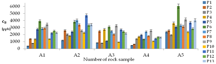
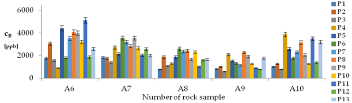
| B concentration in samples after leaching of A1 to A10 rocks using fluids P1 to P13 | |||
 | |||
 | |||
| Model | |||
| cB = −5155 + 35.6t − 549.7TOC − 74.7(TOC)2 − 341.7pH × IS + 25.5pH × TOC + 21.5t × IS + 9.3t × TOC − 211.6G1− 115.4G2 − 60.2G4 − 183.9G5 + 2.4CSB − 81CSMo + 0.06CSSi ± [286.4] c’B = −35.6t − 549.7TOC − 74.7 (TOC)2 − 341.7pH × IS + 25.5pH × TOC + 21.5t × IS + 9.3t × TOC | |||
| R2 | 0.90 | Residual analysis | 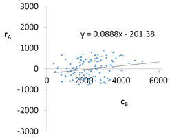 |
| p | <0.000001 | ||
| a | 0.0888 | ||
| α = arctan (a) | 5.1° | ||
| Pearson | 0.30 | ||
| cmin (t = 60 °C) | 1238 ppb | ||
| cmax (t = 60 °C) | 1967 ppb | ||
| cmin (t = 80 °C) | 2181 ppb | ||
| cmax (t = 80 °C) | 3159 ppb | ||
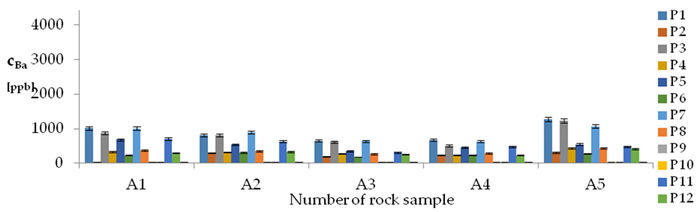
| Ba concentrations in samples after leaching of A1 to A10 rocks using fluids P1 to P13 | |||
 | |||
 | |||
| Model | |||
| cBa = 1664 – 1792pH + 122pH2 + 43.8TOC2 + 157.7pH × IS − 3.14t × TOC − 48.73G2 − 118.41G3 − 271Aw − 0.44CSBa+ 34.44CSLi + 0.276CSMg + 0.00071CSCa ± [168] c’Ba = −1792pH + 122pH2 + 43.8TOC2 + 157.7pH × IS − 3.14t × TOC | |||
| R2 | 0.90 | Residual analysis | 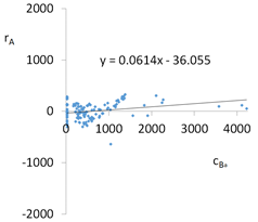 |
| p | <0.000001 | ||
| a | 0.061 | ||
| α = arctan (a) | 3.5° | ||
| Pearson | 0.28 | ||
| c’min (t = 60 °C) | −6741 | ||
| c’max (t = 60 °C) | −5524 | ||
| c’min (t = 80 °C) | −6898 | ||
| c’max (t = 80 °C) | −5527 | ||
| Sr concentration in samples after leaching of A1 to A10 rocks using fluids P1 to P13 | |||
 | |||
 | |||
| Model | |||
| cSr = 11995 − 4001pH + 273.6pH2 + 12.1TOC2 + 2.2pH × t − 4.8pH × TOC − 7t × IS − 72.4IS × TOC + 40.2G2 + 25.6G5 + 129.1Aw + 1.11CSBa − 0.1CSMg − 0.005CSSi + 1.5CSSr ± [134.6] c’Sr = −4001pH + 273.6pH2 + 12.1TOC2 + 2.2pH × t − 4.8pH × TOC − 7t × IS − 72.4IS × TOC | |||
| R2 | 0.95 | Residual analysis | 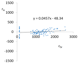 |
| p | <0.000001 | ||
| a | 0.046 | ||
| α = arctan (a) | 2.6° | ||
| Pearson | 0.24 | ||
| c’min (t = 60 °C) | −13910 ppb | ||
| c’max (t = 60 °C) | −12700 ppb | ||
| c’min (t = 80 °C) | −13670 ppb | ||
| c’max (t = 80 °C) | −12310 ppb | ||
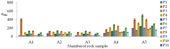
| Mo concentrations in samples after leaching of A1 to A10 rocks using fluids P1 to P13 | |||
 | |||
 | |||
| Model | |||
| cMo = −1002.7 + 37.82t − 15576IS + 207.9TOC + 17.68pH2 − 4.05pH × t + 145.83pH × IS − 3.59t × TOC + 166.94IS × TOC + 3.82G4 + 2.41G5 − 0.38CSB + 10.19CSMo − 0.22CSSr ± [32.7] c’Mo = 37.82t − 15576IS + 207.9TOC + 17.68pH2 − 4.05pH × t + 145.83pH × IS − 3.59t × TOC + 166.94IS × TOC | |||
| R2 | 0.91 | Residual analysis |  |
| p | <0.000001 | ||
| a | 0.069 | ||
| α = arctan (a) | 4.0° | ||
| Pearson | 0.29 | ||
| c’min (t = 60 °C) | 1069 | ||
| c’max (t = 60 °C) | 1695 | ||
| c’min (t = 80 °C) | 1342 | ||
| c’max (t = 80 °C) | 1431 | ||
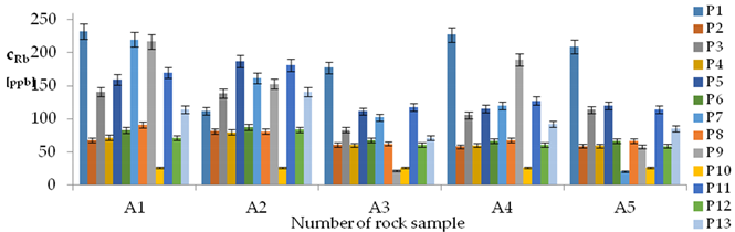
| Rb concentrations in samples after leaching of A1 to A10 rocks using fluids P1 to P13 | |||
 | |||
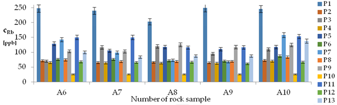 | |||
| Model | |||
| cRb = −77.42 + 1.05t + 462.79 IS + 27.92 pH × IS − 6.49t × IS − 21.88IS × TOC − 0.42G2 + 0.024CSRb ± [18.71] c’Rb = 1.05t + 462.79IS + 27.92pH × IS − 6.49t × IS − 21.88IS × TOC | |||
| R2 | 0.86 | Residual analysis |  |
| p | <0.000001 | ||
| a | 0.102 | ||
| α = arctan (a) | 5.8° | ||
| Pearson | 0.31 | ||
| c’min (t = 60 °C) | 125.9 | ||
| c’max (t = 60 °C) | 227.5 | ||
| c’min (t = 80 °C) | 80.6 | ||
| c’max (t = 80 °C) | 182.2 | ||
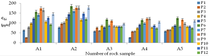
| Li concentrations in samples after leaching of A1 to A10 rocks using fluids P1 to P13 | |||
 | |||
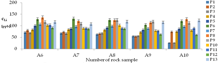 | |||
| Model | |||
| cLi = 500.56 + 78.85pH + 150.00IS − 7.51pH2 + 0.38pH × t − 2.50t × IS − 3.53IS × TOC − 3.03G1 + 1.23G4 − 1.73G5 + 0.41CSLi − 0.0019CSSi + 0.08CSSr − 0.0018CSCa ± [10.66] c’Li = 78.85pH + 150.00IS − 7.51pH2 + 0.38pH × t − 2.50t × IS − 3.53IS × TOC | |||
| R2 | 0.88 | Residual analysis | 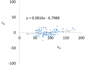 |
| p | <0.000001 | ||
| a | 0.082 | ||
| α = arctan (a) | 4.7 | ||
| Pearson | 0.27 | ||
| c’min (t = 60 °C) | 298.8 | ||
| c’max (t = 60 °C) | 343.6 | ||
| c’min (t = 80 °C) | 341.6 | ||
| c’max (t = 80 °C) | 371.4 | ||
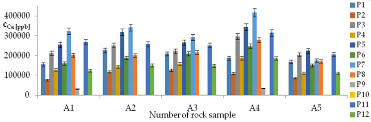
| Ca concentrations in samples after leaching of A1 to A10 rocks using fluids P1 to P13 | |||
 | |||
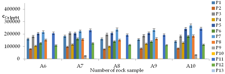 | |||
| Model | |||
| cCa = 1000(3749.56 − 553.95pH − 52.84t + 799.88IS − 83TOC + 39.86TOC2 + 7.84pH × t − 322.63IS × TOC − 1.12G2 − 0.05CSBa − 0.09CSSr + 0.000553CSCa ± [27.07]) c’Ca = 1000(−553.95pH − 52.84t + 799.88IS − 83TOC + 39.86TOC2 + 7.84pH × t − 322.63IS × TOC) | |||
| R2 | 0.90 | Residual analysis | 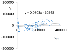 |
| p | <0.000001 | ||
| a | 0.080 | ||
| α = arctan (a) | 4.6° | ||
| Pearson | 0.29 | ||
| c’min (t = 60 °C) | −3897280 | ||
| c’max (t = 60 °C) | −3527670 | ||
| c’min (t = 80 °C) | −3836130 | ||
| c’max (t = 80 °C) | −3172780 | ||
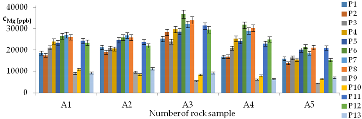
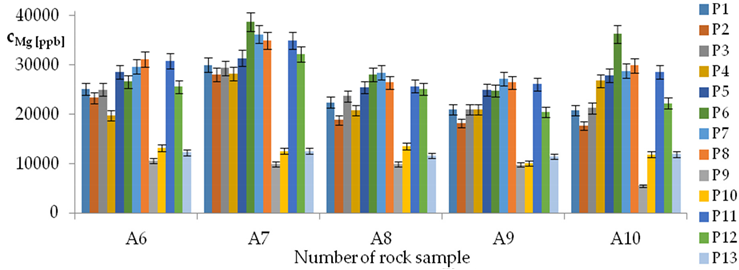
| Mg concentrations in samples after leaching of A1 to A10 rocks using fluids P1 to P13 | |||
 | |||
 | |||
| Model | |||
| cMg = −16117 − 8518pH + 1756.39t − 21296IS + 35845TOC + 3511.7TOC2 + 30118pH × IS − 726.9t × TOC − 294G2 − 775G3 − 459Aw − 8.2CSBa + 1.6009CSMg − 0.1145CSSi ± [2311] cMg = −8518pH + 1756.39t − 21296IS + 35845TOC + 3511.7TOC2 + 30118pH × IS − 726.9t × TOC | |||
| R2 | 0.92 | Residual analysis |  |
| p | <0.000001 | ||
| a | 0.079 | ||
| α = arctan (a) | 4.5° | ||
| Pearson | 0.28 | ||
| c’min (t = 60 °C) | 26676 | ||
| c’max (t = 60 °C) | 57888 | ||
| c’min (t = 80 °C) | 30668 | ||
| c’max (t = 80 °C) | 92144 | ||
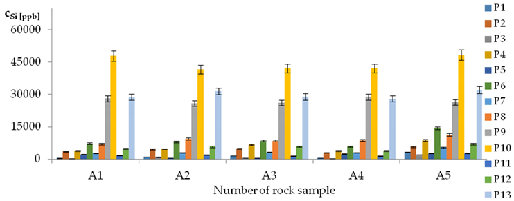
| Si concentrations in samples after leaching of A1 to A10 rocks using fluids P1 to P13 | |||
 | |||
 | |||
| Model | |||
| cSi = −298621 + 9229pH − 35067IS − 6556pH2 + 457TOC2 − 338pH × TOC + 324t × IS − 151.6G1 − 68G5 + 0.0555CSSi ± [2312] cSi = 92297pH − 35067IS − 6556pH2 + 457TOC2 − 338pH × TOC + 324t × IS | |||
| R2 | 0.96 | Residual analysis |  |
| p | <0.000001 | ||
| a | 0.049 | ||
| α = arctan (a) | 2.8° | ||
| Pearson | 0.30 | ||
| c’min (t = 60 °C) | 286589 | ||
| c’max (t = 60 °C) | 316728 | ||
| c’min (t = 80 °C) | 289889 | ||
| c’max (t = 80 °C) | 320028 | ||
| Model | Concentration Operating Range (ppb) | Analysed Concentration Range in MFF (ppb) | ||
|---|---|---|---|---|
| 60 °C | 80 °C | min | max | |
| B | 729 | 978 | 371 | 6044 |
| Ba | 1217 | 1371 | 25 | 4219 |
| Sr | 1210 | 1360 | 125 | 2687 |
| Mo | 626 | 89 | 25 | 760 |
| Rb | 101.6 | 101.6 | 25 | 249 |
| Li | 44.8 | 29.8 | 25 | 186 |
| Ca | 369608 | 663354 | 130 | 417450 |
| Mg | 31212 | 61476 | 4316 | 38782 |
| Si | 30139 | 30139 | 250 | 64153 |
© 2019 by the authors. Licensee MDPI, Basel, Switzerland. This article is an open access article distributed under the terms and conditions of the Creative Commons Attribution (CC BY) license (http://creativecommons.org/licenses/by/4.0/).
Share and Cite
Rogala, A.; Kucharska, K.; Hupka, J. Shales Leaching Modelling for Prediction of Flowback Fluid Composition. Energies 2019, 12, 1404. https://doi.org/10.3390/en12071404
Rogala A, Kucharska K, Hupka J. Shales Leaching Modelling for Prediction of Flowback Fluid Composition. Energies. 2019; 12(7):1404. https://doi.org/10.3390/en12071404
Chicago/Turabian StyleRogala, Andrzej, Karolina Kucharska, and Jan Hupka. 2019. "Shales Leaching Modelling for Prediction of Flowback Fluid Composition" Energies 12, no. 7: 1404. https://doi.org/10.3390/en12071404
APA StyleRogala, A., Kucharska, K., & Hupka, J. (2019). Shales Leaching Modelling for Prediction of Flowback Fluid Composition. Energies, 12(7), 1404. https://doi.org/10.3390/en12071404