Comparative Study of Ramp-Rate Control Algorithms for PV with Energy Storage Systems

Abstract

The high variability of solar irradiance, originated by moving clouds, causes fluctuations in Photovoltaic (PV) power generation, and can negatively impact the grid stability. For this reason, grid codes have incorporated ramp-rate limitations for the injected PV power. Energy Storage Systems (ESS) coordinated by ramp-rate (RR) control algorithms are often applied for mitigating these power fluctuations to the grid. These algorithms generate a power reference to the ESS that opposes the PV fluctuations, reducing them to an acceptable value. Despite their common use, few performance comparisons between the different methods have been presented, especially from a battery status perspective. This is highly important, as different smoothing methods may require the battery to operate at different regimes (i.e., number of cycles and cycles deepness), which directly relates to the battery lifetime performance. This paper intends to fill this gap by analyzing the different methods under the same irradiance profile, and evaluating their capability to limit the RR and maintain the battery State of Charge (SOC) at the end of the day. Moreover, an analysis into the ESS capacity requirements for each of the methods is quantified. Finally, an analysis of the battery cycles and its deepness is performed based on the well-established rainflow cycle counting method.

1. Introduction

It is estimated that PV energy has surpassed the 400 GWp worldwide capacity at the end of 2017 [1]. This represents less than two percent of the worldwide electricity demand, but when compared to the ambition of China alone, of 1300 GW of solar capacity by the year of 2055 [2], illustrates what is yet to come for PV energy systems. However, the increased penetration of solar energy brings new challenges for grid operators, one of which concerns the short-term variability of solar irradiance [3]. This causes high variations in the injected power that can cause serious grid stability issues. To mitigate this problem, power ramp-rate limitation measures have been included in the electrical grid codes of many countries [4]. Generally, these RR limitations are defined on a second or minute time frame or even in both. In addition, the maximum allowable RR can be defined as a percentage of the plant capacity or as a defined set of power. Some examples are the grid code of Ireland (EirGrid), which states a positive ramp up to 30 MW/minute and Hawaii (HECO), ± 2 MW/minute [5]. For Germany [6] and Puerto Rico (PREPA) [5], a maximum ramp-rate of 10%/minute of the rated PV power is considered. Other grid codes also quantify the maximum allowable ramp-rate in the order of seconds. For example, in Denmark [7], a maximum power ramp-rate of 100 kW/s is required.

Several RR calculation methods are defined in the technical literature [5], some examples are: the difference between two endpoints of a 60-second interval, the difference between the minimum/maximum values of a considered interval and the difference between two points at each second interval, Figure 1. Despite the different RR calculation methods presented, few clarifications exist on the grid codes on how to perform this calculation in practice.

To allow ramp-rate limitation, PV plants are required to have additional power in reserve. In practice, this is possible by e.g., operating the PV plant below the rated capacity. This is achieved by e.g., disconnecting a portion of the PV arrays, effectively reducing the injected power to the grid [8]. Other possibility relies on constraining the maximum power point (MPP) by modifying the traditional maximum power point tracker (MPPT) algorithms [9,10].

Another solution is the use of battery energy storage systems (BESS) [11], which can absorb or inject power in order to compensate for the ramp-rate violation. The continuous decrease in battery prices [12], along with the recent policies and incentives for increasing the application of energy storage for new and existing power plants, makes BESS an increasingly attractive solution. Besides PV power fluctuation smoothing, battery systems present other inherent possibilities [13,14], such examples are: (i) bulk energy services: energy time-shift (arbitrage), avoid renewable curtailment; (ii) ancillary services: frequency regulation, voltage support; (iii) transmission/distribution services: upgrade deferral, outage mitigation [13,14].

Previous research on PV smoothing algorithms with BESS falls under two main categories: filter type methods and gradient methods. However, in this work, only filter type methods are addressed. In [15], the traditional moving average (MA) algorithm is implemented on a PV with a lead acid battery storage. A 30-day continuous test is performed, showing the capability of the MA algorithm in smoothing the PV fluctuations. In [16], the MA algorithm performance is again demonstrated in simulation and in a full-scale 500 kW implementation. The system presents two independent BESS systems, one for dispatch, and the other dedicated for power smoothing. The controls were implemented via SCADA and a 15-minute time window is considered for the MA algorithm.

In [17], a second smoothing strategy based on the exponential moving average (EMA) is presented. The algorithm considers a 10-minute window in tandem with a hydrogen storage system. The EMA algorithm proves to be capable of regulating the PV fluctuations giving more weight to the more recent data points, when compared to the MA.

The work in [18] proposes a smoothing technique based on a first order low-pass filter (LPF). The filtered PV output power serves as a reference for the BESS to eliminate the higher power fluctuations. The method is reported to have the capability of limiting the PV power fluctuations within acceptable values.

In [19], a second order LPF (2-LPF) for PV power smoothing is presented, which is capable of suppressing the higher PV power fluctuations. Moreover, its superior performance when compared to the single first order LPF, is discussed.

In [20], a ramp-rate based gradient control is presented. The main difference of this algorithm compared with the others is that it does not filter the PV output power. It works by compensating (injecting or absorbing) power depending on the instantaneous derivative of the PV output. It also has the advantage of not requiring any previous tuning being independent of past irradiance data.

Despite the different smoothing methods and algorithms presented, there is a lack of inter comparison and benchmarking of these methods. Thus, this paper intends to be an overview and to characterize each of the methods under the same circumstances. Special attention is given into the methods capability in limiting the PV power RR for a full operational day. Moreover, this paper also aims to provide useful information on which RR method would utilize best a certain BESS. For that reason, focus is given on the battery state of charge, number of cycles and their corresponding cycle depths something, which is very often omitted in most publications on smoothing methods. By characterizing the battery performance under each of the smoothing methods, a better battery usage can be achieved and the optimum smoothing method selected. This inevitably improves the overall system operation and reliability [21].

2. Power Smoothing Methods

In this work, four smoothing methods, reported in the literature as: moving average (MA), exponential moving average (EMA), low-pass filter (LPF), second order low-pass filter (2-LPF) are considered for analysis. The basic principle of these filter type methods is to filter the high fluctuations in the PV generated power, which arise due to partial shading of the PV arrays. These smoothing methods generate a battery power reference that opposes the PV power variations. The result is an injected grid power within the acceptable RR limits. The general implementation of the filter type smoothing methods can be observed in Figure 2 for a traditional double-stage PV+BESS.

2.1. Moving Average (MA)

The moving average, as previously discussed, is one of the most common smoothing methods. It works by averaging the previous PV power (P_pv) values for a given period of time w. It is mathematically represented at a k^th instant, by:

$$P_{batt}{}^{*}\left(k\right)=\frac{{{\displaystyle \sum }}_{i=0}^{w-1}{P}_{pv}\left(k-i\right)}{w}-P_{pv}\left(k\right)$$

(1)

Depending on the averaging period, the PV power smoothing will be more or less significant. In addition, irrespectively of the window length, all samples have equal weight. Previous publications [22] and [20] proposed a moving average window of 20 minutes for a 4 kW and 1 kW PV system, respectively, while, in [23] and [16], a 16-minute and 15-minute moving average for a 10 MW and 500 kW PV plant are considered.

2.2. Exponential Moving Average (EMA)

The exponential moving average, similar to the MA, relies on previous sampled data. However, besides including the window length, it also applies a smoothing factor (also known as forgetting factor) α. It is represented by:

$$P_{batt}{}^{*}\left(k\right)=\alpha \left[P_{pv}\left(k\right)+{\left(1-\alpha \right)}^n{P}_{pv}\left(k-n\right)\right]-P_{pv}$$

(2)

where n = {0,1,2, …, $w$-1} and the factor α indicates how much weight is given on the past data points. The higher the value of α, the more equal is the weight between previous data points and the more recent ones.

2.3. First Order Low-Pass Filter (LPF)

The LPF method works by reducing the high frequency components presented in the PV output power, and so producing a power reference for the battery. The discrete implementation of the LPF using Forward Euler approximation is given by:

$$H\left(z\right)=\frac{\left(T/T_f\right)z^{-1}}{1+\left(T/T_f-1\right)z^{-1}}$$

(3)

where T_f is the filter time constant and T represents the sampling period. A high T_f results in higher smoothing profiles, whereas a low one will allow higher order frequencies to pass. The filter is tuned based on the irradiance pattern, which may not ensure an RR of 10% all the time, as the grid code demand. In [18], the output power of a 150 kW PV system is smoothed by an LPF with time constant of 120-seconds.

2.4. Second Order Low-Pass Filter (2-LPF)

The second order LPF was also tested as a power smoothing method. Adding a steeper filtering can help reduce the system requirements in terms of battery capacity. The discrete implementation of the 2-LPF using Forward Euler approximation is given by:

$$H\left(z\right)=\frac{T^2{\omega }_n{}^2{z}^{-2}}{1+\left(2\zeta {\omega }_{n}T-2\right)z^{-1}+\left(1-2\zeta {\omega }_{n}T+T^2{\omega }_n{}^2\right)z^{-2}}$$

(4)

where ω_n is the filter natural frequency, ζ is the damping ratio and T represents the sampling period.

3. Methodology

3.1. Comparison and Assumptions

The different PV power smoothing methods are evaluated for the simulation system of Figure 2, considering the irradiance profile illustrated in Figure 3. For an easier evaluation of the system, the simulated irradiance profile was reduce to the period above 50 W/m2, eliminating the night and as well the sunrise and sunset.

In order to proper evaluate the different smoothing techniques, the following practical features were considered:

• Ability to limit the RR to 10% per minute of the rated power,
• Battery SOC level and status at end of the day,
• Battery energy level,
• Battery Cycles.

The analysis is divided into three main parts. First, the power smoothing methods are evaluated based on the ability to limit the RR to 10% per minute of the rated power and to maintain the SOC at end of the day. This is accomplished by varying the corresponding smoothing methods parameters (e.g., window average interval, filter time constant and natural frequency) until an optimum operation is possible. This ensures a fair comparison, in which each smoothing method is compared for the minimum battery requirement that accomplishes the limit of 10%/minute of RR. In addition, it is desirable that the battery regains its initial SOC at the end of the day. This ensures that the battery contains enough energy to start operating the next day. It also guarantees that the total generated power is indeed provided to the grid rather than storage, improving the system operation.

Secondly, the different SOC levels and battery energy are compared. This indicates how much energy requirements each method needs in its operation. It also maps which percentage of the battery energy is used and at which time of the day.

Finally, the battery number of cycles and their deepness under each of the smoothing methods in a full operation day are assessed, based on the rainflow counting method. This allows for better mapping the battery performance and its corresponding lifetime [21].

In order to simulate the system as precisely as possible, but also not increasing the complexity and simulation time, the following assumptions were considered:

• The DC/DC converters and inverter are simulated as average models, since the focus of this work is not in the dynamic response.
• The PV array considers a constant temperature, invariant during the system operation.
• The battery capacitance is treated as constant during the system simulation. This is considered as the degradation in the battery capacitance is not significant for a 1-day operation.
• The effect of the temperature is not taken into account on the battery model.

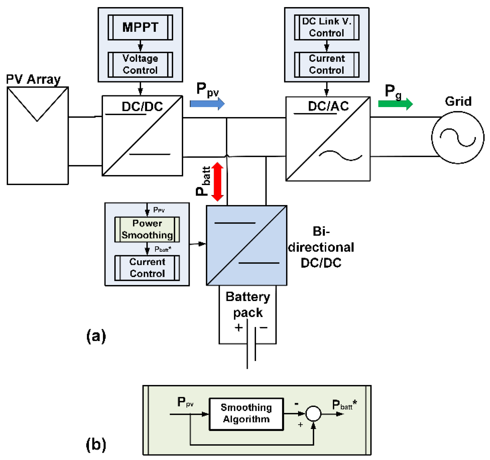
3.2. System Description

The traditional PV+BESS system can be observed in Figure 2a. It is generally composed of: (i) a PV voltage boost stage responsible for the PV MPP tracking; (ii) an inverter stage implementing the grid connection and DC link voltage control; and (iii) a bi-directional DC/DC charge regulator of the battery pack. In Figure 2b, the generic structure of the filter based smoothing algorithms is presented.

To evaluate the operation of the different smoothing methods, the system of Figure 2a was simulated in Simulink/PLECS environment. The simulation model is composed of a PV array model based on the four-parameter Shockley diode equations and parameterized from the datasheet in [24], corresponding to a 0.9 kWp BPMSX120 PV string. The two DC/DC converters are implemented as average models. One converter is responsible for the PV boost stage, and controlled by a maximum power point tracking (MPPT) based on the Perturb & Observe (P&O) method [25,26]. The second converter is responsible for the bi-directional charge regulator of the battery pack. The inverter is implemented as an average model and parameterized based on Danfoss FC 302 VLTs, rated at 2.2 kW. An outer DC-bus voltage controller and an inner PR current controller are responsible for the correct inverter operation. The inner controller is tuned for a phase margin (PM) of 48 deg with a bandwidth of 900 Hz. The outer loop presents a bandwidth ten times smaller.

The battery pack model was implemented based on the empirical model for Li-Ion batteries presented in [27], which follows Shepherd´s equation for battery voltage estimation [28]. The battery was assumed to be the same size for all the power smoothing methods under test. The methodology for sizing the battery follows [29], considering an oversizing term of 1.2 related to the 10%–90% SOC limits for battery operation, and is the following:

$$E_{rated}=1.2\times 2\times \frac{0.9\times P^r{}_{PV}}{1800{\eta }^{out}{}_{batt}}\left[\frac{2700}{r_i}-\tau -\tau \times e^{\frac{-5400}{\tau \times r_i}}\right]\approx 300Wh,$$

(5)

where E_rated is the rated battery energy requirement in [Wh], P^r_PV the rated PV power and considered 0.9 [kW], η^out_batt is the battery efficiency of 0.94, r_i the ramp limit of 10 [%/min] and $\tau$ the PV plant time constant, considered 0 due to the small size of the PV plant. The result is a total battery energy of 300 Wh, obtained with 51 series connected 1.5 Ah Sanyo UR18650WX battery cells [30] The parameters of

Table 1. Battery parameters.

Parameters	Li-Ion Battery
Battery constant voltage E0 [V]	201.5
Internal resistance R [Ω]	0.255
Battery capacity Q [Ah]	1.5
Polarization resistance/constant K [Ω or V/(Ah)]	0.76
Exponential zone amplitude A [V]	8.21
Exponential zone time constant inverse B [A/h]	12

are then obtained for this battery, based on the extracting parameters procedure presented in [27].

3.3. Analysis Conditions

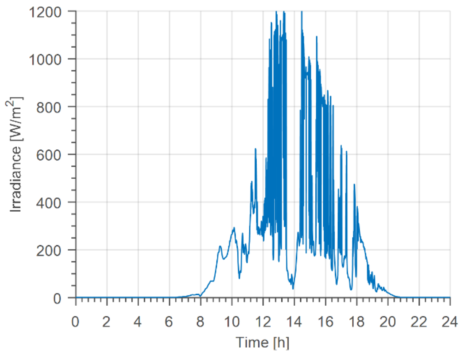
3.3.1. Irradiance Profile

To evaluate the different smoothing strategies, a 1-day irradiance profile obtained from the Aalborg university weather station was selected, Figure 3. The irradiance was measured by a calibrated crystalline silicon reference cell (Si-RS485TC-WT-v-MB) from IMT solar, positioned with a 45° tilt, south orientation, with a 1 Hz sampling rate. The irradiance profile was characterized considering the solar variability score (VS_RRdist) presented in [31]. Since the different smoothing methods and the battery sizing are heavily dependent on the irradiance profile, using the solar variability as a characterization tool, allows for better extending this work into other practical scenarios. The VS_RRdist is calculated by:

$$V{S}_{RRdist}\left(\Delta t\right)=100\times [R{R}_0\times P(\left|R{R}_{\Delta t}\right|>R{R}_0)]$$

(6)

where ∆t is the timescale considered, RR₀ is the maximum allowed ramp-rate in percentage and $P\left(\left|R{R}_{\Delta t}\right|>R{R}_0\right)$ is the probability that any ramp is bigger than RR₀. For this work, the irradiance profile of Figure 3 with a solar variability score equal to 250 classified as “high”, the second highest in a six-scale chart [31], is considered. This ensures that the smoothing techniques and the associated parameters (window average interval, filter time constant and natural frequency) can be applied to an area with a variability score lower or equal to 250.

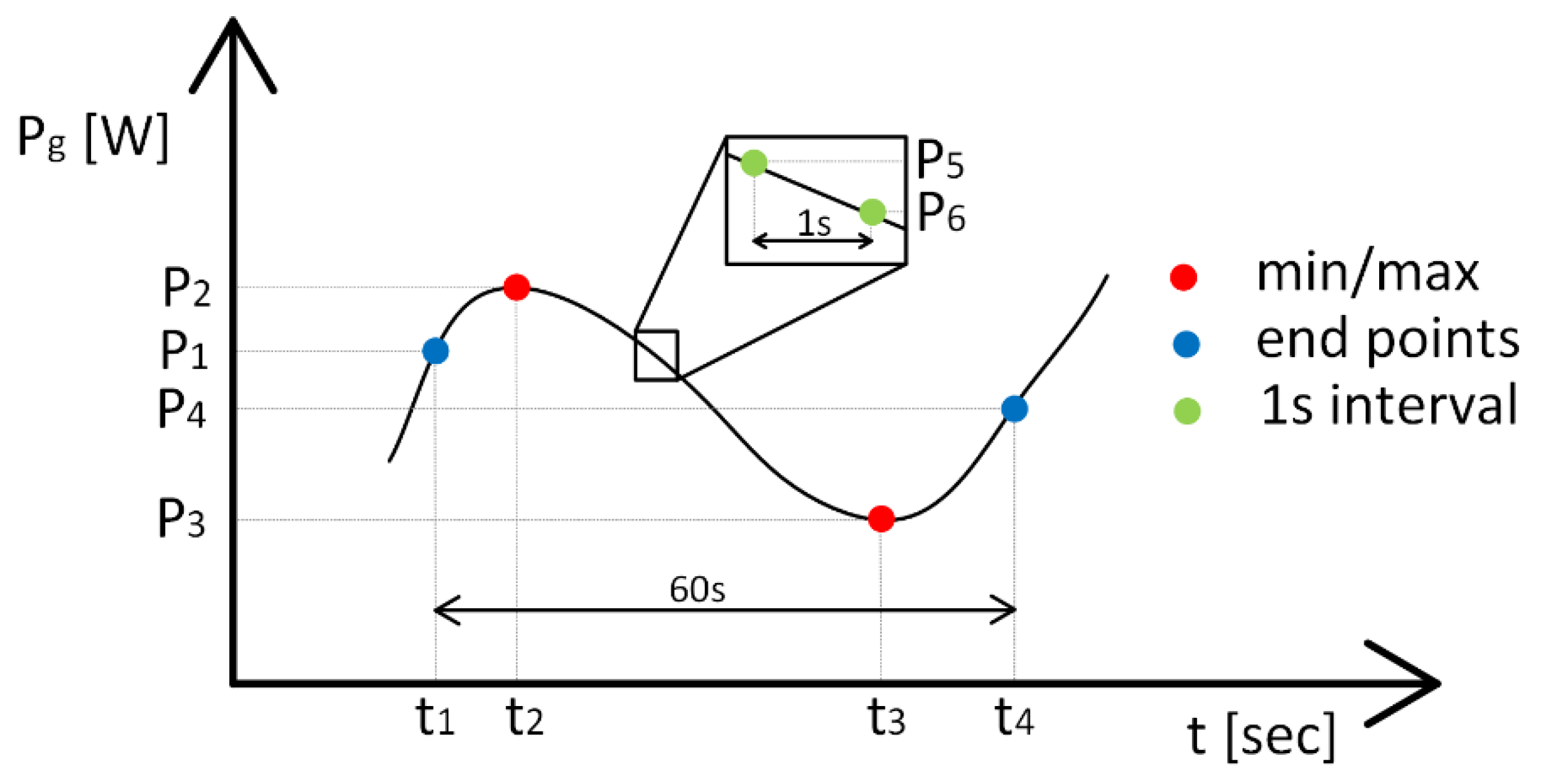
3.3.2. Ramp-Rate Calculation

Different methods for PV generation ramp-rate calculation have been reported in the literature. The two most common are the difference between two end points or the difference between the maximum and minimum points of the same considered interval [5]. In addition, depending on the grid code, the RR calculation may be presented on instantaneous values or per minute values. In this work, the RR calculation is considered to be the difference between two end points of a given 60-second interval as presented in Equation (6):

$$RR\left(t\right)=\frac{P\left(t\right)-P\left(t-60\right)}{t\left(t\right)-t\left(t-60\right)}$$

(7)

where P(t) and t(t) are the grid power and time at the current instant and the index (t − 60) represents the time interval 60 seconds ago.

In addition, a limit of 10% of the PV plant rated power is considered as the maximum RR permitted.

4. Results

4.1. Power Smoothing Evaluation

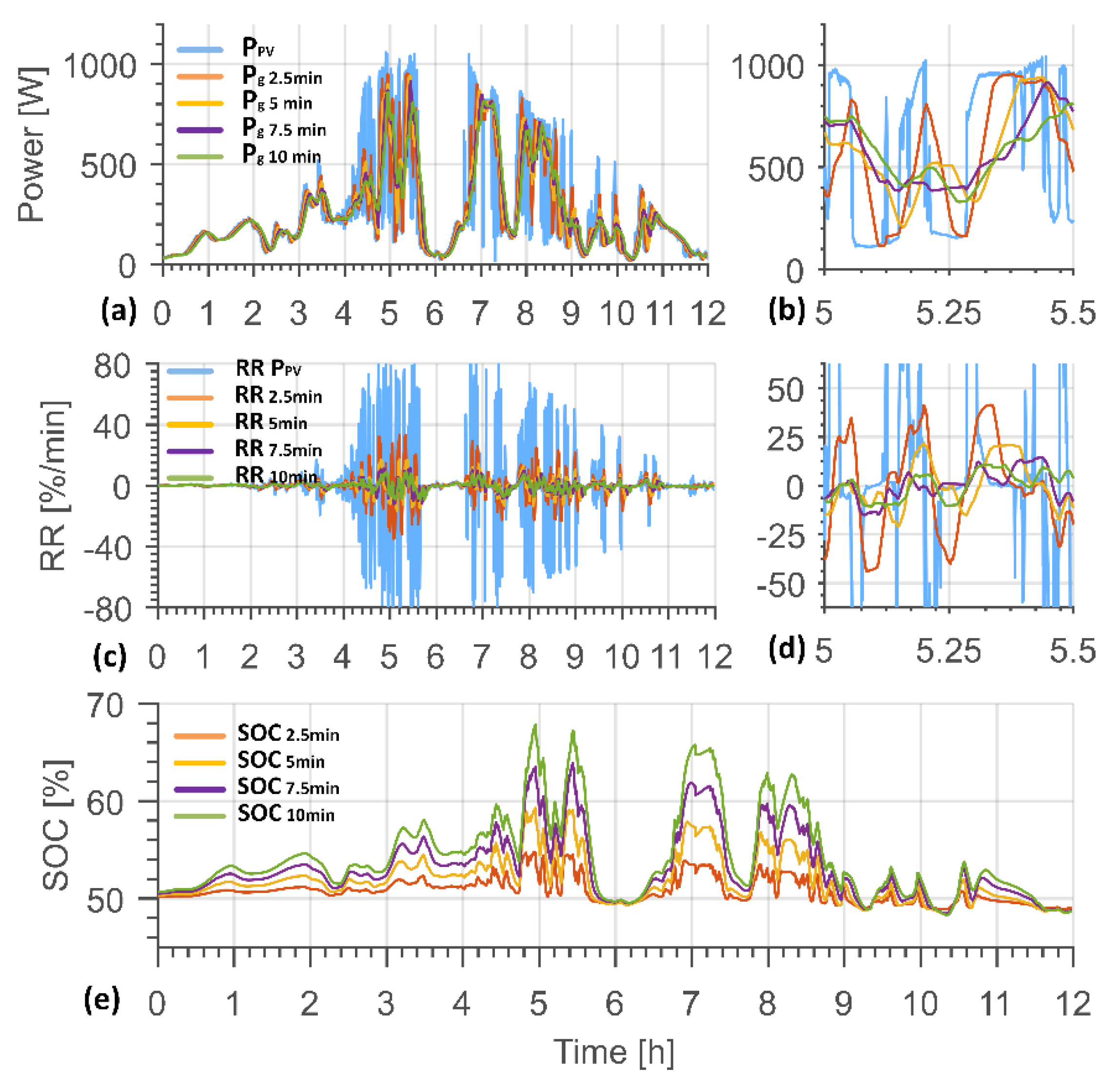
4.1.1. Moving Average (MA)

In Figure 4, the impact of the MA smoothing strategy for a 2.5-minute to a 10-minute window length is presented. As can be observed in Figure 4a the increase in the MA window length reduces the amplitude of the grid power oscillations. This is special noticeable from the maximization of Figure 4b. The reduction in the power fluctuations is more evident from Figure 4c,d where a quantification of the ramp-rate in %/minute is shown. For a window length greater or equal to 10-minutes, the algorithm proves sufficient in maintaining the RR below 10%/minute of the rated power. Figure 4e also shows the increase in the SOC variation as the MA window increases, which comes from the fact that more power is being absorbed as the result of limiting the power fluctuations. This algorithm is also capable of guaranteeing that the initial and final SOC are at identical levels.

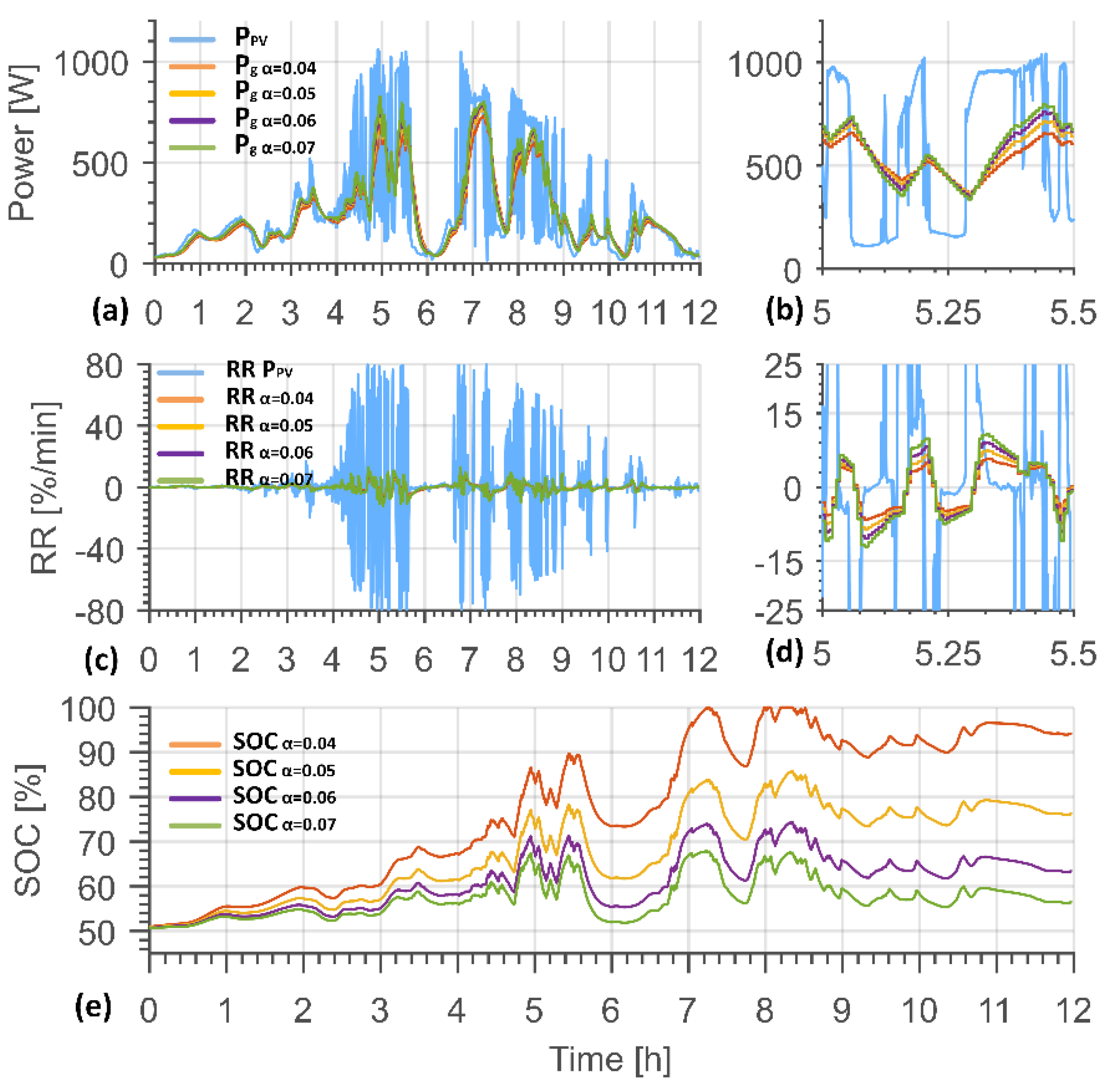
4.1.2. Exponential Moving Average (EMA)

In Figure 5 an analysis of the EMA smoothing technique for a considered window length of 20-minutes and a smoothing factor from 0.04 to 0.07 is presented. As can be observed on Figure 5a,b the use of the EMA reduces the grid power fluctuations. Moreover, from Figure 5c,d the increase in α increases the ramp-rate value. Actually, for an α value below or equal to 0.04 the algorithm proves to be capable of reducing the oscillations to 10%/minute of the rated power. From Figure 5e it can be observed that the EMA requires for the battery to absorb more energy to achieve the required 10% RR per minute, when compared to the MA method. In fact, for an α = 0.04 the battery becomes saturated, reaching a SOC level of 100%. It is then not possible for the battery to process all the required energy. In addition, the algorithm fails to regain the SOC to its initial position at the end of the day. This indicates that a great percentage of the generated power by the system is not indeed injected to the grid, but storage.

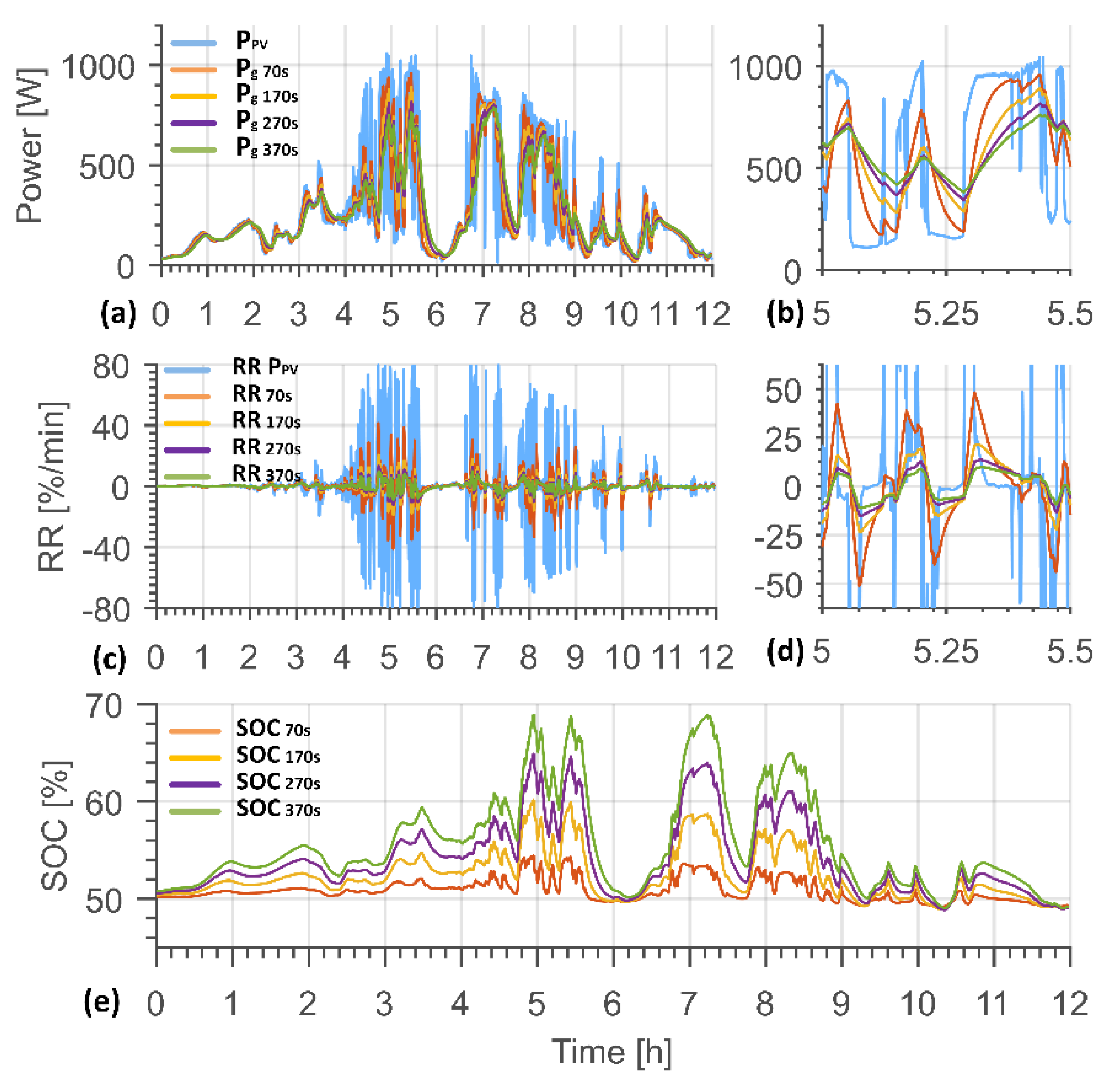
4.1.3. First Order Low-Pass Filter (LPF)

In Figure 6 an analysis of the LPF smoothing method for different time constants was performed. From Figure 6a,b the increase in the filter time constant from 70-seconds until 370-seconds has reduce the amplitude of the fluctuations on the power injected to the grid. This is quantified by Figure 6c,d where the increase in the filter time constant has reduced the maximum value of RR from about 40%/minute at 70-seconds to 10%/minute at 370-seconds, complying with the maximum allowed RR limit. Moreover, from Figure 6e the restitution of the SOC to its original value at the end of the day can be depicted, similarly to what previously observed from the MA smoothing method.

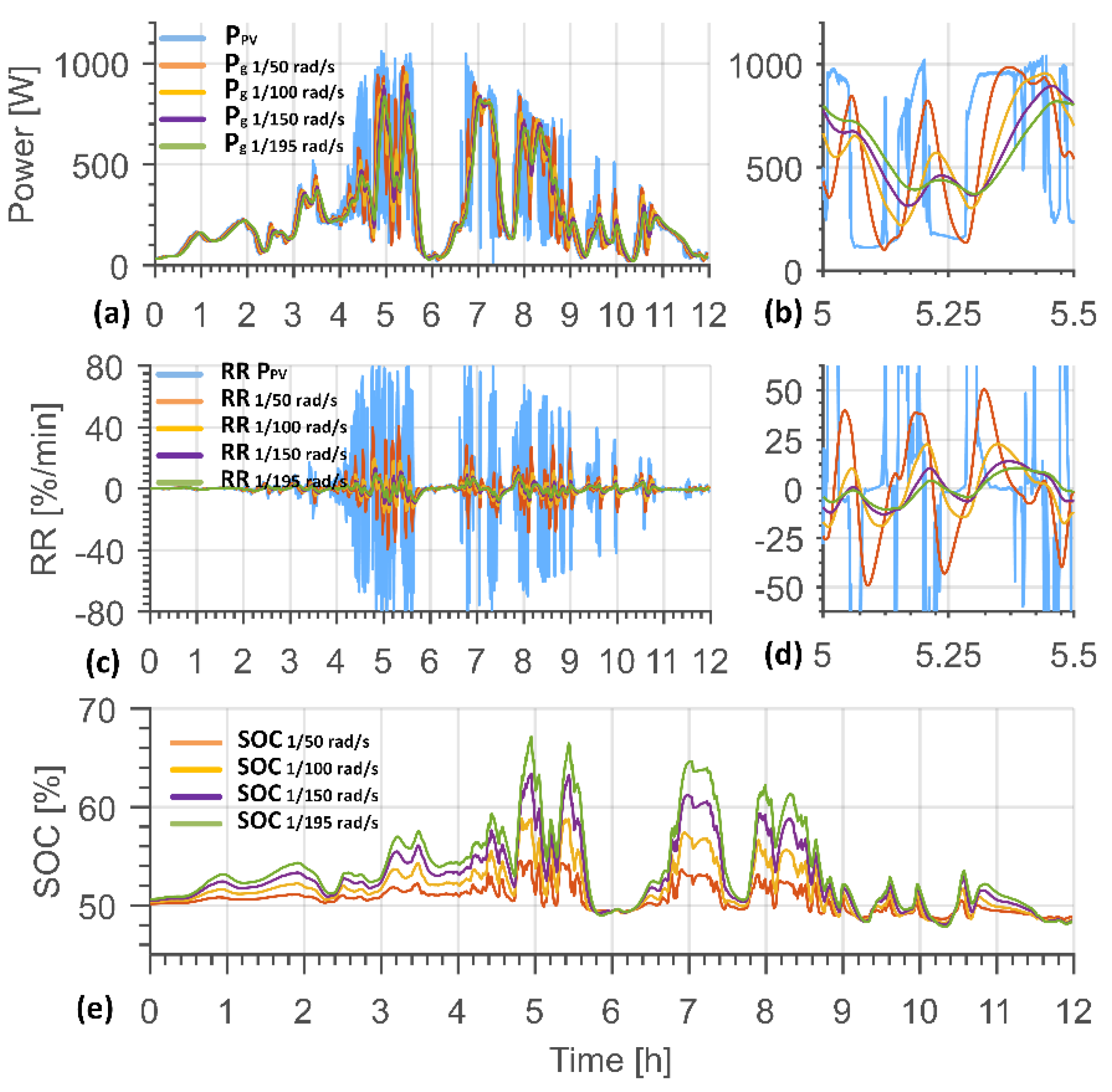
4.1.4. Second Order Low-Pass Filter (2-LPF)

From Figure 7 the study of the 2-LPF smoothing method for different natural frequencies and considering a constant damping factor of 0.707 is presented. In Figure 7a,b the reduction of the power fluctuations with the decrease in the filter natural frequency is demonstrated. Moreover, from Figure 7c,d the decrease in RR with the decrease in the natural frequency is again observed, where for a ω_n of 1/50 rad/s and 1/196 rad/s the system reduces the power fluctuations from 50%/minute to less than 10%/minute. Similar to the LPF and MA methods the 2-LPF is capable of maintaining the SOC at the end of the day closer to its initial value Figure 7e.

4.2. Energy and Power Exchange with Battery

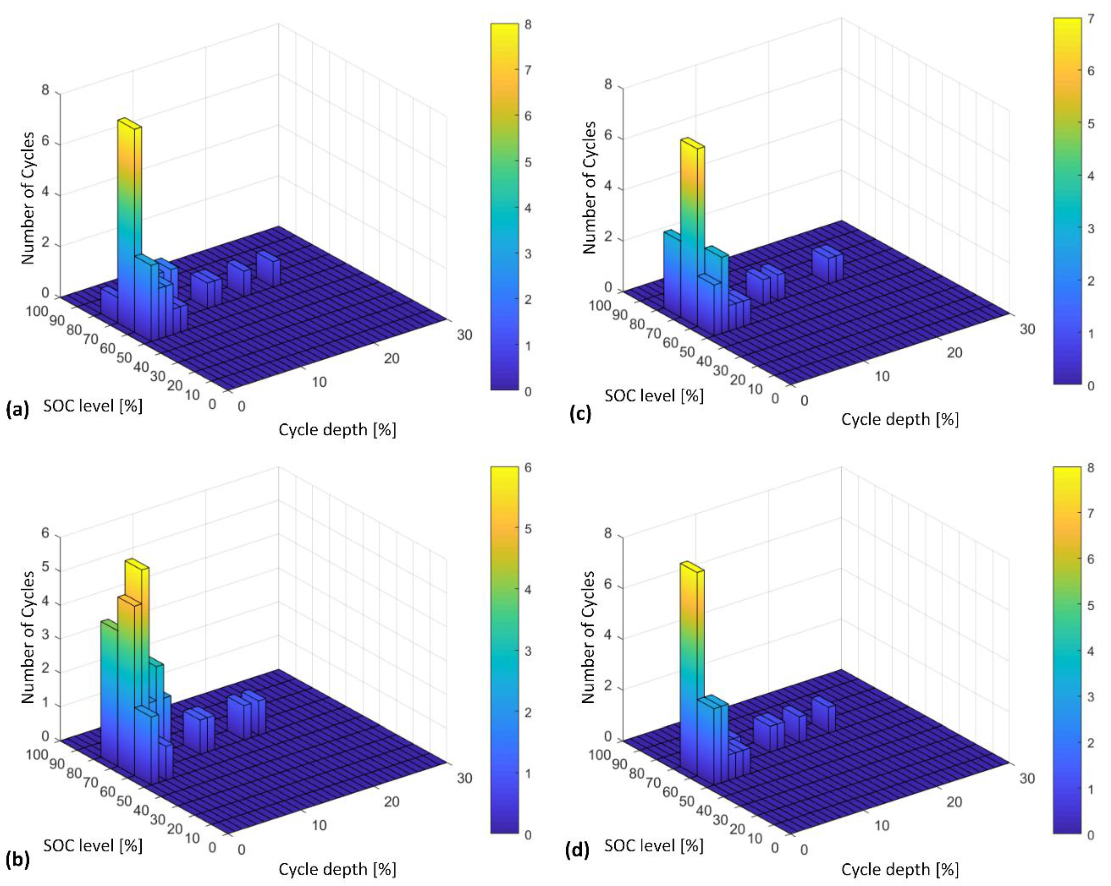
For understanding the battery performance under each of the four smoothing methods, Figure 8 was compiled. The data for each of the methods is collected for the condition where the RR value is 10%/minute. This means MA method with window length of 10-minutes, EMA method with α = 0.05 and window length of 20-minutes, LPF with time constant of 370-seconds and 2-LPF method with 1/195 rad/s of natural frequency.

From Figure 8a,b is possible to understand that the second order LPF exchanges less energy with the battery compared to the other three methods. This represents a SOC saving of 1.5% when compared to the MA method and close to 3% when compared to the LPF method. When expressed in energy, the saving is closed to 4.5 Wh and 9 Wh for the MA and LPF smoothing methods respectively.

From Figure 8a it is also possible to observe the incapability of the EMA method in bringing the SOC back to its initial state. This originates excess energy to be storage in the battery, which indicates that a portion of the generated PV power was not injected back into the grid. The result is a poor performance of the EMA smoothing method from a battery utilization perspective.

As for the two most common smoothing methods, LPF and MA their performance in battery energy utilization is more similar, Figure 8a. Although, the MA method still reports a lower SOC being an overall superior smoothing method.

It is also interesting to compare the bandwidth of the first and second order LPF for the condition where the RR of 10%/minute is met. This corresponds to a bandwidth of 0.0027 rad/s and 0.0051 rad/s for the first and second order LPF respectively. This helps to understand the difference in SOC of Figure 8a for both these methods, the first order LPF by presenting a lower bandwidth is required to filter more of the PV generated power, which directly indicates that more energy is processed in order to smooth the power fluctuations.

In addition, from Figure 8 the battery power of the four smoothing methods is presented. As can be observe the 2-LPF presents marginally higher peak power when compared to the MA and LPF methods, Figure 8c. However, it also presents faster dynamics, Figure 8d, reducing the battery power faster to zero then the other three methods, this reduces the amount of energy being processed for power smoothing, leading to improvements in battery usage.

4.3. Battery Cycles

One key aspect in a battery system is the battery lifetime. This is highly dependent on the number of cycles and as well as on the cycle’s depths. For this reason, the selection of the smoothing method has to consider not only the battery capacity but also the degradation caused by these cycles. In order to quantify the cycles number and their deepness, the rainflow cycle counting method, proposed in [32] for fatigue analysis and reproduce for battery applications, is used. Similarly to the previous results, the data in this analysis is collected for the condition where the RR value is 10%/minute.

In Figure 9 a comparison of the number of cycles, their depth along with the corresponding SOC level (i.e., average SOC value of the cycle), for the four smoothing methods in study, is presented. These results are obtained for a rainflow cycle counting method with a 1% SOC resolution.

Considering the previous obtained results, the EMA smoothing method, Figure 9b failed to regain the SOC to its initial condition. For this reason a direct comparison, in terms of battery cycles, with the other smoothing methods is not practical. However, this method presents a sum of 23 cycles with a cycle depth of 1% to 4% and a sum of 6 cycles with a cycle depth of 5% to 18%. The other three methods present a sum of 21, 23 and 19 cycles between 1% to 4% of cycle depth for the MA Figure 9a, LPF Figure 9c and 2-LPF Figure 9d, respectively. As for higher depth cycles the three previous smoothing methods present a sum of 7, 6 and 7 cycles between 5% and 20% of cycle depth, respectively. Moreover, the cycle depth of the two higher cycles is 16% and 20% for the MA, 19% and 20% for the LPF and 15% and 19% for the 2-LPF. Based on these results, it can be concluded that the 2-LPF presents fewer cycles with lower depth, when compared to the two remaining methods.

4.4. Lifetime Analysis

The lifetime estimation of Li-Ion batteries is directly related with the gradual deterioration of their performance parameters, mainly capacity fade and power capability, which are also referred to as ageing [21]. The mechanisms for battery ageing are normally related with the deterioration of its internal components, especially at the electrode–electrolyte interface, active materials and composite electrode. These ageing phenomena inevitably decrease the battery reliability and performance, placing the system operation at risk.

The factors for which the ageing mechanisms occur have a variety of sources (temperature, SOC, cycle depth and number of cycles) and are presented both at cycling and during storage [21].

On what ageing during storage concerns, it normally occurs for high temperature and high SOC levels [21]. This is exactly what occurs for the EMA smoothing method Figure 8a, where a high SOC level is presented after a full operation day. This means that, a high level of energy is storage during the night period where the battery does not operate. It is then expected that a battery under the EMA smoothing method presents a shorter lifetime when compared to the other three smoothing methods.

As for the ageing during cycling, this is related with the number of cycles and especially, with the depth of this same cycles. On what this is concern, it is expected that the 2-LPF method presents a longer lifetime than the MA or the LPF. This is due to the 2-LPF smoothing method presenting overall less number of cycles, and also the depth of the higher cycles being less when compared to the MA and LPF, Figure 9.

5. Conclusions

This work presents an in-depth analysis of the most common methods for PV power smoothing with BESS. An analysis, based on a simulation, under the same conditions of irradiance profile was performed. This profile is characterized by a high solar variability, which helps map the results obtained under regions with same conditions of irradiance variability. The obtained results were divided into three main groups. First, in what concerns the capability of limiting the RR to 10%/minute of the rated power, all methods were capable of performing this feature. However, the EMA smoothing method required more battery capacitance, and was not capable of bringing the SOC to its original position. This is highly desirable as ensures that the PV power produced is provided to the grid with minimal losses and the system is ready to restart operation the next day. Related to the battery energy, the second order LPF proves to utilize less battery capacity, when compared to the MA and first order LPF. It also presents the least number of cycles and with reduced deepness when compared to the other smoothing methods. This method is then expected to present a higher lifetime.

Despite the through assessment of the different smoothing methods under a single irradiance day, more understanding has to be gained on the battery entire life operation. Future research intends to build a lifetime model to better understand these issues.

References

1. Tsao, R. Strong Chinese Market to Push Annual Global Photovoltaic Demand Above 100 Gigawatts for 2017. 20 January 2018. Available online: https://press.trendforce.com/press/20170914-2962.html (accessed on 8 April 2019).
2. Yang, X.J.; Hu, H.; Tan, T.; Li, J. China’s renewable energy goals by 2050. Environ. Dev. 2016, 20, 83–90. [Google Scholar] [CrossRef]
3. Yang, Y.; Enjeti, P.; Blaabjerg, F.; Wang, H. Wide-scale adoption of photovoltaic energy: Grid code modifications are explored in the distribution grid. IEEE Ind. Appl. Mag. 2015, 21, 21–31. [Google Scholar] [CrossRef]
4. Energinet.dk. Technical Regulation 3.2.2 for PV Power Plants with a Power Output Above 11 kW; Energinet.dk: Denmark, 2015; pp. 1–96. Available online: https://en.energinet.dk/Electricity/Rules-and-Regulations/Regulations-for-grid-connection (accessed on 8 April 2019).
5. Booth, S.; Gevorgian, V. Review of PREPA Technical Requirements for Interconnecting Wind and Solar Generation; National Renewable Energy Laboratory: Golden, CO, USA, 2013.
6. BDEW Bundesverband der Energie- und Wasserwirtschaft e.V. Technische Richtlinie, Erzeugungsanlagen Am Mittelspannungsnetz; BDEW: Germany, June 2008; p. 138. Available online: https://www.bonn-netz.de/Einspeisung/Vertraege/Stromeinspeisevertraege/Anlage-3-Technische-Richtlinien-Erzeugungsanlagen-am-Mittelspannungsnetz.pdf (accessed on 8 April 2019).
7. Energinet.dk. Technical Regulation 3.2.2 for PV Power Plants Above 11 kW; Energinet.dk: Denmark, 2016; pp. 1–108. Available online: https://en.energinet.dk/Electricity/Rules-and-Regulations/Regulations-for-grid-connection (accessed on 8 April 2019).
8. Sangwongwanich, A.; Yang, Y.; Blaabjerg, F. A cost-effective power ramp-rate control strategy for single-phase two-stage grid-connected photovoltaic systems. In Proceedings of the 2016 IEEE Energy Conversion Congress and Exposition (ECCE), Milwaukee, WI, USA, 18–22 September 2016. [Google Scholar]
9. Omran, W.A.; Kazerani, M.; Salama, M.M.A. Investigation of Methods for Reduction of Power Fluctuations Generated From Large Grid-Connected Photovoltaic Systems. IEEE Trans. Energy Convers. 2011, 26, 318–327. [Google Scholar] [CrossRef]
10. Ina, N.; Yanagawa, S.; Kato, T.; Suzuoki, Y. Smoothing of PV system output by tuning MPPT control. Electr. Eng. Jpn. 2005, 152, 10–17. [Google Scholar] [CrossRef]
11. Chen, J.; Li, J.; Zhang, Y.; Bao, G.; Ge, X.; Li, P. A Hierarchical Optimal Operation Strategy of Hybrid Energy Storage System in Distribution Networks with High Photovoltaic Penetration. Energies 2018, 11, 389. [Google Scholar] [CrossRef]
12. Chediak, M. The Latest Bull Case for Electric Cars: The Cheapest Batteries Ever; Bloomberg Technology. 2017. Available online: https://www.bloomberg.com/news/articles/2018-07-13/wework-tells-employees-meat-is-permanently-off-the-company-menu (accessed on 5 April 2019).
13. Xu, X.; Casale, E.; Bishop, M.; Oikarinen, D. Application of new generic models for PV and battery storage in system planning studies. In Proceedings of the Power & Energy Society General Meeting, Chicago, IL, USA, 16–20 July 2017. [Google Scholar]
14. Faessler, B.; Schuler, M.; Preibinger, M.; Kepplinger, P. Battery Storage Systems as Grid-Balancing Measure in Low-Voltage Distribution Grids with Distributed Generation. Energies 2017, 10, 2161. [Google Scholar] [CrossRef]
15. Hund, T.D.; Gonzalez, S.; Barrett, K. Grid-tied PV system energy smoothing. In Proceedings of the 2010 35th IEEE Photovoltaic Specialists Conference, Honolulu, HI, USA, 20–25 June 2010; pp. 2762–2766. [Google Scholar]
16. Ellis, A.; Schoenwald, D.; Hawkins, J.; Willard, S.; Arellano, B. PV output smoothing with energy storage. In Proceedings of the 2012 38th IEEE Photovoltaic Specialists Conference, Austin, TX, USA, 3–8 June 2012; pp. 1523–1528. [Google Scholar]
17. Tesfahunegn, S.G.; Ulleberg, Ø.; Vie, P.J.S.; Undeland, T.M. PV fluctuation balancing using hydrogen storage—A smoothing method for integration of PV generation into the utility grid. Energy Procedia 2011, 12, 1015–1022. [Google Scholar] [CrossRef]
18. Liu, H.; Peng, J.; Zang, Q.; Yang, K. Control Strategy of Energy Storage for Smoothing Photovoltaic Power Fluctuations. IFAC-PapersOnLine 2015, 48, 162–165. [Google Scholar] [CrossRef]
19. Nikolov, D.N. Power Ramp Rate Reduction in Photovoltaic Power Plants Using Energy Storage. Master’s Thesis, Aalborg University, Aalborg, Denmark, 2017. [Google Scholar]
20. Alam, M.J.E.; Muttaqi, K.M.; Sutanto, D. A novel approach for ramp-rate control of solar PV using energy storage to mitigate output fluctuations caused by cloud passing. IEEE Trans. Energy Convers. 2014, 29, 507–518. [Google Scholar]
21. Stroe, D. Lifetime Models for Lithium Ion Batteries Used in Virtual Power Plants. Ph.D. Thesis, Aalborg University, Aalborg, Denmark, September 2014. [Google Scholar]
22. Kakimoto, N.; Satoh, H.; Takayama, S.; Nakamura, K. Ramp-rate control of photovoltaic generator with electric double-layer capacitor. IEEE Trans. Energy Convers. 2009, 24, 465–473. [Google Scholar] [CrossRef]
23. Puri, A. Optimally smoothing output of PV farms. In Proceedings of the 2014 IEEE PES General Meeting|Conference & Exposition, National Harbor, MD, USA, 27–31 July 2014. [Google Scholar]
24. Sera, D. Real-Time Modelling, Diagnostics and Optimised MPPT for Residental PV Systems; Aalborg University: Aalborg, Denmark, 2009. [Google Scholar]
25. Hohm, D.P.; Ropp, M.E. Comparative study of maximum power point tracking algorithms using an experimental, programmable, maximum power point tracking test bed. In Proceedings of the Conference Record of the Twenty-Eighth IEEE Photovoltaic Specialists Conference, Anchorage, AK, USA, 15–22 September 2000; pp. 1699–1702. [Google Scholar]
26. Spataru, S.; Martins, J.; Stroe, D.; Sera, D. Test Platform for Photovoltaic Systems with Integrated Battery Energy Storage Applications. In Proceedings of the 2018 IEEE 7th World Conference on Photovoltaic Energy Conversion (WCPEC), Waikoloa Village, HI, USA, 10–15 June 2018; pp. 2–7. [Google Scholar]
27. Tremblay, O.; Dessaint, L.-A. Experimental validation of a battery dynamic model for EV applications. World Electr. Veh. J. 2009, 3, 289–298. [Google Scholar] [CrossRef]
28. Shepherd, C.M. Design of primary and secondary cells II. An equation describing battery discharge. J. Electrochem. Soc. 1965, 112, 657–664. [Google Scholar] [CrossRef]
29. Moghaddam, I.; Chowdhury, B. Battery Energy Storage Sizing With Respect to PV-induced Power Ramping Concerns in Distribution Networks. In Proceedings of the 2017 IEEE Power & Energy Society General Meeting, Chicago, IL, USA, 16–20 July 2017; Volume 5. [Google Scholar]
30. Panasonic. Lithium Ion UR18650WX, 2012. Available online: https://na.industrial.panasonic.com/sites/default/pidsa/files/ur18650wx4.pdf (accessed on 7 April 2019).
31. Lave, M.; Broderick, R.J.; Reno, M.J. Solar variability zones: Satellite-derived zones that represent high-frequency ground variability. Sol. Energy 2017, 151, 119–128. [Google Scholar] [CrossRef]
32. Amzallag, C.; Gerey, J.P.; Robert, J.L.; Bahuaud, J. Standardization of the rainflow counting method for fatigue analysis. Int. J. Fatigue 1994, 16, 287–293. [Google Scholar] [CrossRef]
Figure 1. Ramp-rate calculation methods: difference between two endpoints of a 60-second interval RR = (P4 − P1)/(t4 − t1), difference between the minimum/maximum values of a considered interval RR = (P3 − P2)/(t3 − t2), difference between two points at each second interval RR = (P6 − P5)/1s.
Energies 12 01342 g001
Figure 2. Traditional PV+BESS system: (a) circuit representation; (b) power smoothing methods implementation principle.
Energies 12 01342 g002
Figure 3. Irradiance profile considered in this study, obtained from the Aalborg University weather station.
Energies 12 01342 g003
Figure 4. PV+BESS system with the applied MA smoothing technique for a 2.5-minute to 10-minute window: (a) Ppv and Pg; (b) Ppv and Pg (zoom); (c) Ramp-Rate in % per minute; (d) Ramp-Rate in % per minute (zoom); (e) state-of-charge.
Energies 12 01342 g004
Figure 5. PV+BESS system for 20-minute of applied EMA smoothing technique with α = 0.04 to 0.07: (a) Ppv and Pg; (b) Ppv and Pg (zoom); (c) Ramp-Rate in % per minute; (d) Ramp-Rate in % per minute (zoom); (e) state-of-charge.
Energies 12 01342 g005
Figure 6. PV+BESS system for 70 seconds to 370 seconds of applied LPF smoothing technique: (a) Ppv and Pg; (b) Ppv and Pg (zoom); (c) Ramp-Rate in % per minute; (d) Ramp-Rate in % per minute (zoom); (e) state-of-charge.
Energies 12 01342 g006
Figure 7. PV+BESS system for 1/50 rad/s to 1/195 rad/s of applied 2-LPF smoothing technique: (a) Ppv and Pg; (b) Ppv and Pg (zoom); (c) Ramp-Rate in % per minute; (d) Ramp-Rate in % per minute (zoom); (e) state-of-charge.
Energies 12 01342 g007
Figure 8. Comparison of the four smoothing methods: (a) SOC; (b) SOC (zoom); (c) battery power; (d) battery power (zoom).
Energies 12 01342 g008
Figure 9. Battery cycle counting for: (a) MA; (b) EMA; (c) LPF and (d) 2-LPF, based on the rainflow cycle counting method.
Energies 12 01342 g009