Abstract
Hydraulic fracturing is a widely used production stimulation technology for conventional and unconventional reservoirs. The cohesive element is used to explain the tip fracture process. In this paper, the cohesive zone model was used to simulate hydraulic fracture initiation and propagation at the same time rock deformation and fluid exchange. A numerical model for fracture propagation in poro-viscoelastic formation is considered. In this numerical model, we incorporate the pore-pressure effect by coupling fluid diffusion with shale matrix viscoelasticity. The numerical procedure for hydraulically driven fracture propagation uses a poro-viscoelasticity theory to describe the fluid diffusion and matrix creep in the solid skeleton, in conjunction with pore-pressure cohesive zone model and ABAQUS was used as a platform for the numerical simulation. The simulation results are compared with the available solutions in the literature. The higher the approaching angle, the higher the differential stress, tensile stress difference, injection rate, and injection fluid viscosity, and it will be easier for hydraulic fracture crossing natural fracture. These results could provide theoretical guidance for predicting the generation of fracture network and gain a better understanding of deformational behavior of shale when fracturing.
1. Introduction
Unconventional reservoirs, such as shale, coal seam and tight-gas sand, are highly reliant on hydraulic fracturing to increase the production. Although it is difficult to exploit, these low-permeability reservoirs contain considerable hydrocarbon resources such as Marcellus Shale [1], Barnett Shale [2] and Eagle Ford Shale [3]. The purpose of hydraulic fracturing is to open natural fracture and increase the number of flow paths, to connect the natural fractures in the reservoir with the hydraulic fractures, opening the existing natural fractures, and increasing the path volume in the fractures. Natural fracture plays an important role in hydraulic fracturing such as increasing shale gas flow path, enhancing productivity, and reducing propped fracture length [3]. Natural fractures have an important influence in hydraulic fracturing. It cannot only affect the propagation of fracturing in reservoirs, but it also affects the efficiency of hydraulic fracturing treatment. The benefit of natural fractures is that it can expand the flow path volume and increase the production of hydrocarbons. On the negative side, it may cause additional resources to leak. Therefore, understanding of how the hydraulic fractures interact with natural fractures is necessary and is beneficial to our future simulations and improvements. Overall, continuous research on hydraulic fracturing is necessary and worthwhile. Hydraulic fracture intersection with natural fracture was investigated through both laboratory and mine-back experimental approaches [4,5,6,7]. When hydraulic fractures intersect with natural fractures, there are three different developments. Hydraulic fractures cross over natural fractures without changing the volume or shape of natural fractures; hydraulic fractures divert into the natural fracture and expand the volume of the flow path; hydraulic fractures enter natural fractures and form a complex fracture network structure.
Biot first proposed viscoelastic theory to study the linear viscoelasticity and anisotropy of porous media [8]. The influence of the permeability on the deformation and the settlement problem of the loaded column was discussed. A micromechanical method for explaining the theory of pore viscoelasticity of Biot is proposed by Abousleiman et al. [9]. The problem of drilling under plane-strain deformation is discussed and the effects of combined poro- and visco-elasticity are investigated. Simakin and Ghassemi [10] put forward another poro-viscoelastic model by considering the relaxation of the deviatoric stress and the symmetric effective stress. These constitutive models can be used to simulate the coupling process between fluid flow and creep deformation of matrix rocks, but they cannot be directly applied to simulate hydraulic fracturing, especially the interaction of hydraulic fracturing with natural fractures. Hydraulic fracturing is a complex process and it contains rock deformation, fracturing fluid flow, and fracture imitation and propagation. Linear Elastic Fracture Mechanics (LEFM), which is known as a method to describe fracture mechanics in brittle rock, made outstanding contributions. However, for soft rock, LEFM has no advantage. Under formation temperature and pressure, the brittle rock in shale exhibits ductility after hydraulic fracturing treatments. Therefore, it may not be the best choice to use elastic theory to analyze the shale failure.
The cohesive zone model (CZM) is a model in fracture mechanics in which fracture formation is considered to be a gradual phenomenon. The separation of the surface involved in the crack occurs on the extended crack tip or cohesive region and resists traction by bonding. By using CZM, the crack initiation and propagation in many kinds of materials could be predicted and it makes a detailed description of fracture process zone become possible [11]. CZM assumed the fracture process zone may be separated by traction-separation law (TSL), which is determined by the material of the fracture treatment zone. The presence of cohesive traction eliminates the singularity of the crack tip, and this singularity significantly affects the convergence of the solution. The standard model for describing the fracture tip processing region is the assumed bond portion extending between the fracture surfaces until they break at an appropriate level of traction [12,13]. CZM has great advantages in predicting crack propagation orientation in different kinds of materials (such as metals, concrete, and rocks [14]). Furthermore, it has been used for simulating hydraulic fracture interactions with natural fracture [15,16,17].
In this paper, using this method to simulate the hydraulic fracturing from initiation and propagation, the rock deformation and fluid exchange between porous infiltrated media and fractures are being coupled. The cohesive element is used to explain the tip fracture process. The numerical procedure for hydraulically driven fracture propagation uses a poro-viscoelasticity theory to describe the fluid diffusion and matrix creep in the solid skeleton. Moreover, pore-pressure CZM and ABAQUS was used as a platform for the numerical simulation.
2. Poro-Viscoelastic Model
2.1. Poro-Viscoelastic Model
When the rock material is subjected to an external load greater than the long-term strength, and the external stress conditions are constant, the rock deformation gradually increases with time. The rock incurs creep when the internal strain reaches the accelerated creep threshold, and the strain will eventually reach the strength of the fracture and finally break. It is generally considered that the rock has a long-term effect on the external constant load creep phenomenon, so the viscoelastic model is suitable. The How law is used to model the stress and strain for an elastic material. Nevertheless, viscoelastic materials generally show elasticity and viscous deformation over time. The rock deformation and fluid diffusion are involved in the physical process and influence each other. The poro-viscoelasticity theory has been developed and used for the fluid-rock coupling effect [18]. In this paper, the Maxwell model will be used to illustrate the viscoelasticity shown in Equation (1):
Poro-viscoelasticity is the synthesis of poro-elasticity and viscoelasticity. Biot [14] pioneered the approach by using the correspondence principle, which allows for straightforward conversion from elastic to viscoelastic behavior. The constitutive equations for a poro-elastic rock are regarded as:
where K is rock bulk Young’s modulus, G is shear Young’s modulus, ɑ is the Biot’s effective stress coefficient which measures the ability of the pore pressure to resist compressional stresses, M is the Biot’s Modulus. The corresponding total stress components added to pore pressure of the fluid (p) value is the components of effective stress tensor.
The difference between the constitutive equation of poro-viscoelasticity and that of poro-viscoelasticity is the viscous term (see right-hand side of Equation (1)). The deviatoric and symmetric components of stress act on the time developed by the viscous behavior, by adding these two elements using the finite method. A fully coupled hydro-mechanical process, the increment of total stress at the current stage is showed as:
where is the pseudo-stress tensor which denotes the viscous influence of the strain history. Besides the above equation, a fluid diffusion equation should be used,
where k is the permeability. Equations (5) and (6) show a combination for poro-viscoelasticity. They can be used to simulate fluid flow under plane-strain conditions as well as the interaction between viscoelastic deformation of rock mass and fluid flow during mechanical processes.
In the ABAQUS platform, it assumes that the time domain viscoelasticity is determined by a Prony series expansion. In the Prony series the parameters are defined for each term. On the other hand, ABAQUS can calculate the terms in the Prony series using time-dependent creep test data, time-dependent relaxation test data, or frequency-dependent cyclic test data. The parameters used in Prony series are acquired from nonlinear regression based on power-law equations acquired from experimental data [19].
2.2. Compare Poro-Elastic Model to Poro-Viscoelastic Model
In numerical simulation, a 2D plane-strain crack propagation problem is considered. The formation is regarded as homogeneously poro-viscoelastic. Only half of the model is meshed due to its symmetry. The initial perforated crack is located at the center, while the predefined crack path is located on the x-axis. The model is subjected to far-field in situ stress, as shown in Figure 1.
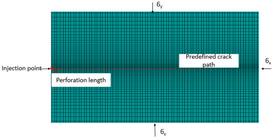
Figure 1.
2D crack in plane-strain condition.
To investigate the effect of poro-viscoelastic formation on fracture propagation, results from poro-viscoelastic formation are compared with poro-elastic formation. The input parameters are the same except for cohesive strength and viscosity. The parameters used for numerical simulations are presented in Table 1. Figure 2 presents fracture propagation geometry in poro-elastic and poro-viscoelastic formations, respectively. Poro-viscoelastic model fracture width is larger than poro-elastic, while the half fracture height is smaller than poro-elastic. Since the hydraulic energy is partly dissipated during the subsequent ongoing viscous deformation, more time is needed to build up the required input to initiate fracture growth. In the meantime, the fracture is widened due to decaying modulus of the bulk. The model shows that the poro-viscoelastic is differently poro-elastic so this principle for shale needs to be considered in our simulation.

Table 1.
All the parameters used in numerical simulation.
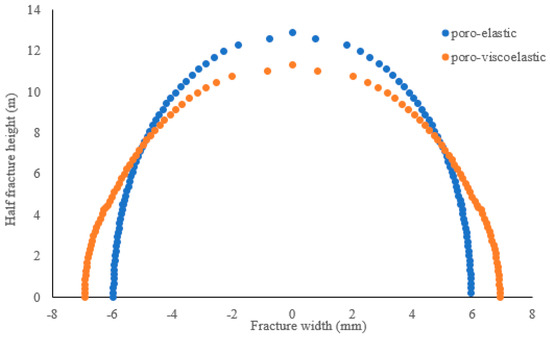
Figure 2.
Fracture geometry with time.
3. Model Setup
3.1. Cohesive Zone Model
The interaction between hydraulic fracture and natural fracture from initiation to the propagation was modeled in the CZM by introducing a layer of elements (possible path) with zero thickness. Fully modeling the hydraulic fracturing process requires solving a coupled system of governing equations [20,21]. A well is drilled and then a hydraulic fracture with injection fluid enters the reservoir. The fracture process zone (unbroken cohesive zone) is defined within the upper and lower surfaces in Figure 3. The fracturing fluid is filled with fracture where no traction from shale fracture exists. The bilinear model is used in the CZM. Three stages can be observed in the process of opening fracture. (1) At first, the opening increases at the tip. Following with this change, the traction of cohesive element also increases. Traction changes from 0 to Tmax, traction in this point is the largest tensile strength, the opening at this point is called critical opening (δn), and interface bonding degradation starts at this point. (2) As the opening increases, traction decreases with the opening until 0; during this time, the cohesive element is continually damaged. The opening when traction reaches 0 is called failure opening (δt). (3) Exceeding this point, the cohesive element was totally damaged. Because of the fluid flow, the opening will continually increase.
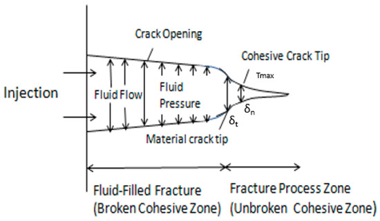
Figure 3.
The hydraulic fracture tips.
Cohesive using stiffness degradation to describe the damage evolution process of the element:
The D is the damage index to the elastic linear material
where δm is the maximum effective relative displacement, δ0 is normal loading displacement and δf is shear loading displacement.
There is a fluid flow in the viscous surface gap. By Newtonian rheology, we assume that the fluid is incompressible. The lubrication equations control the tangential flow in the tip, which is formulated from Poiseuille’s law:
The ordinary flow is explained:
where pt is the top surface pore pressures, pb is bottom surfaces of the fracture pore pressure, and Ct and Cb define the corresponding fluid leak-off coefficients.
3.2. Interaction Model Setup
ABAQUS is finite-element software for structural and field analysis in the mechanical, civil, and electronics industries, which mainly include CAE, STANDARD, and EXPLICIT [22]. In this program, a hydraulic fracture is injected and interacts with a natural facture in rock, and is analyzed and simulated by it. Existing cracks appear to be closed, and there is no initial separation in the entire path. The Newtonian fluid, which is incompressible, continues to enter the fracture at a constant injection flow rate (Q0) and causes the initiation and expansion of fractures created by hydraulic fracturing. There is no fluid leak-off through the impermeable surfaces of the fracture, so that the simulation only models the flow in the fracture radius direction. Six-node coupled displacement and pore-pressure axisymmetric cohesive elements are used to model the fracture, and the rock is modeled with 4-node axisymmetric elastic elements. The cohesive elements at the injection point are defined as initially open to allow entry of the fluid, which makes the process of initial flow and fracture growth come true. Since the model we built is for tensile fractures, the cohesive element is continually undergoing damage until 0, and fails in purely normal deformation conditions without considering shear deformation. Four categories of parameters were set up, including Young’s modulus in rock properties; tensile strength; maximal horizontal stress and minimum horizontal stress in in situ stress; and viscosity and injection rate in pumping parameters. Some of these values are not fixed; a preliminary simulation can be performed by setting initial values, and then the results can be changed by adjusting the values.
First, we establish the model and determine the included angle through the establishment of the model also determined here; 60° is taken as an example (Figure 4). The model is then given basic properties such as Young’s modulus and Poisson’s ratio. After determining the nature of the rock to be simulated, assembly integration was performed. Different densities of mash are needed because it can facilitate convergence of calculation results. We define the initial conditions by step, keeping the ground stress balanced, then inject the fluid, set the time and boundary conditions, and start crack propagation.
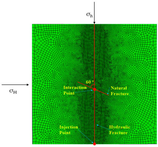
Figure 4.
The mesh of hydraulic fracture interacts with natural fracture at 60°.
4. Results and Discussion
Hydraulic fracture geometry is largely dependent on the different parameters and the different parameter sizes have different impacts on hydraulic fracture geometries. The variable includes in situ stress, interaction angle, tensile strength, fracturing fluid injection rate, and fracturing fluid injection fluid viscosity. During every parameter analysis, we only change one parameter; nevertheless, the other parameters remain unchanged according to the basic model in Table 2.
Table 2.
Input Parameters.
4.1. Interaction Angle
The interaction angle has enough effects on the hydraulic fracture propagation. By changing the angle, the influence of different angles on the interaction between HF (Hydraulic Fracture) and NF (Natural Fracture) can be obtained. In this paper, change of NFs is compared at 30 degrees, 45 degrees, 60 degrees, and 75 degrees, respectively, under the same other conditions. To verify the results of fracture intersection, the comparison between modeling results and the indoor experiment are shown in Figure 5 [7]. From the picture, the different legend means the result of HF intersection of NF. It can be seen that numerical simulation results and the lab experimental results are in good agreement. This demonstrates that the CZM could simulate HF intersecting with NF. As is shown in Figure 5, the smaller the interaction angle, the more fractures produced by hydraulic fracturing tend to divert into the NFs and lead to an opening in the NFs. Moreover, for smaller angles of intersection, HF is more likely to divert and propagate along the obtuse angle branch of NF. With high approach angle, the HF is more likely to cross the NF.

Figure 5.
The model verification with experimental results.
4.2. In Situ Stress
The in situ stress difference is an essential parameter in hydraulic fracturing design. The horizontal stresses are the result of the poro-elastic deformation of the rocks plus externally applied tectonic forces. The maximum horizontal stress and the minimum horizontal stress always control the HF initiation and propagation. In this simulation, the maximal horizontal stress is 8 MPa, and we then change the minimal horizontal stress in 8 MPa, 5 MPa, and 2 MPa, respectively in the three cases, as well as keeping the other parameters consistent with the basic model to observe the relationship between HF and NF. It can be seen in Figure 6 that the greater the stress difference, the more easily HFs tend to cross through NFs. The smaller the stress difference, the more conducive to the expansion of NFs [15,16].
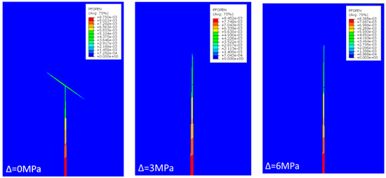
Figure 6.
Crack geometry under different in situ stress.
4.3. Crack Tensile Strength
Rock tensile strength is a measure of the force required to achieve its point of failure. The tensile strength is a characteristic property of the rock and the crack tensile strength obviously less than the shale. In the simulation, the shale tensile strength is taken as 6 MPa, while the crack tensile strength is 1 MPa, 3 MPa, and 5 MPa, respectively, in the three cases. The different tensile strength NF means different strength of NF effect on HF propagation. The simulation results in Figure 7 show the HF conquers the shale tensile strength, the HF initiation, and propagation. Therefore, the tensile stress difference ∆St = rock tensile strength—crack tensile strength. When the shale tensile strength is larger than the crack tensile strength, it is easy to generate the bi-wing fracture. When the shale tensile strength is moderately larger than the crack tensile strength, it is easy to generate the single-wing fracture. When the shale tensile strength is almost equal to the crack tensile strength, HF crosses NF [23].
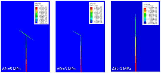
Figure 7.
Crack geometry in difference tensile strength.
4.4. Fracturing Fluid Injection Rate
Injection rates have a great impact on fracture geometry, as shown in Figure 8, and they influence fracture patterns. In this simulation, the fracturing fluid injection rate is taken as 3 m3/min, 6 m3/min, and 12 m3/min. The crack geometries of the three examples are described in Figure 8. When the injection rate is high, HF is more likely to cross NFs, and at the same time fill the entire crack. This increases not only the fracture length but also the fracture width when increasing the fracturing fluid injection rate.
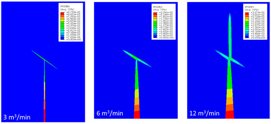
Figure 8.
Crack geometry in different fracturing fluid injection rate.
4.5. Fracturing Fluid Injection Viscosity
When injecting hydraulic fluid into the shale, the fracturing fluid penetrates the rock gap and crack, generating fracturing fluid loss. The fracturing fluid loss is mainly decided by fracturing fluid viscosity. In this simulation, the fracturing fluid viscosity is taken as 4 mPa∙s, 8 mPa∙s, and 16 mPa∙s. The simulation results in Figure 9 show the higher fracturing fluid viscosity increase fluid flow resistance and promote the establishment of a cake on the hydraulic rupture surface, thereby reducing fluid loss [24]. When the viscosity is high, HF is more likely to cross NFs. Injecting in a low viscosity is helpful for forming a complex network structure [25].
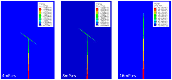
Figure 9.
Crack geometry in different fracturing fluid injection viscosity.
5. Conclusions
In this paper, we developed a fully coupled poro-viscoelastic fracture propagation model to investigate the characteristics of hydraulic fracturing in shale formation. The numerical simulation adopted is the finite-element method and detailed implementation steps are presented. Simulations of poro-viscoelastic fracture propagation confirm the generally accepted notion that creep behavior has a detrimental effect on hydraulic fracturing efficiency. From the analysis, it is found that fractures propagating in poro-viscoelastic formation tend to be wider yet shorter than that in poro-elastic formation, which is mainly due to viscous energy dissipation.
By using a cohesive finite-element model, different factors that effect HF interacting with NF have been investigated and clearly simulated. On the one hand, the interaction between HF and NF can promote the expansion of flow paths; on the other hand, it may lead to an extra leak-off. Using TSL, the tip of the fracture process is described in detail. From five different aspects, the interaction between HF and NF has been analyzed. As the angle of interaction continues to decrease (from 75°), HF changes from passing through NF to diverting to NF; reducing the difference between the maximum horizontal stress and the minimum horizontal stress to reduce the differential stress can also achieve a similar effect; injecting in a suitable rate or viscosity is helpful to make full use of NFs and improve the fracturing effect.
Author Contributions
Y.S. wrote the paper and designed the model, Z.C. conceive the problem, H.Y. editing paper suggestion and D.W. analyzed the data, Y.Z. provide paper editing suggestion.
Funding
The authors would like to give their sincere gratitude to the National Science Foundation of China (Grant No. 51804033), China Postdoctoral Science and Foundation (Grant No. 2018M641254), Beijing Postdoctoral Research Foundation (Grant No. 2018-ZZ-045).
Conflicts of Interest
The authors declare no conflict of interest.
References
- Pommer, L.; Gale, J.F.; Eichhubl, P.; Fall, A.; Laubach, S.E. Using structural diagenesis to infer the timing of natural fractures in the Marcellus Shale. In Proceedings of the Unconventional Resources Technology Conference, Denver, CO, USA, 12–14 August 2013; Society of Exploration Geophysicists, American Association of Petroleum: Tulsa, OK, USA, 2013; pp. 1639–1644. [Google Scholar]
- Patel, H.; Johanning, J.; Fry, M. Borehole microseismic, completion and production data analysis to determine future wellbore placement, spacing and vertical connectivity, Eagle Ford shale, South Texas. In Proceedings of the SEG Technical Program Expanded Abstracts 2014, Denver, CO, USA, 26–31 October 2014; Society of Exploration Geophysicists: Tulsa, OK, USA, 2014. [Google Scholar]
- Fan, L.; Martin, R.B.; Thompson, J.W.; Atwood, K.; Robinson, J.R.; Lindsay, G.J. An integrated approach for understanding oil and gas reserves potential in eagle ford shale formation. In Proceedings of the Canadian Unconventional Resources Conference, Calgary, AB, Canada, 15–17 November 2011; Society of Petroleum Engineers: Richardson, TX, USA, 2011. [Google Scholar]
- Cipolla, C.L.; Warpinski, N.R.; Mayerhofer, M.; Lolon, E.P.; Vincent, M. The relationship between fracture complexity, reservoir properties, and fracture treatment design. In Proceedings of the SPE Annual Technical Conference and Exhibition, SPE Annual Technical Conference and Exhibition, Denver, CO, USA, 21–24 September 2008; Society of Petroleum Engineers: Richardson, TX, USA, 2008. [Google Scholar]
- Blanton, T.L. An experimental study of interaction between hydraulically induced and pre-existing fractures. In Proceedings of the SPE Unconventional Gas Recovery Symposium, Pittsburgh, PA, USA, 16–18 May 1982; Society of Petroleum Engineers: Richardson, TX, USA, 1982. [Google Scholar]
- Warpinski, N.R.; Teufel, L.W. Influence of geologic discontinuities on hydraulic fracture propagation (includes associated papers 17011 and 17074). J. Pet. Technol. 1987, 39, 209–220. [Google Scholar] [CrossRef]
- Zhou, J.; Chen, M.; Jin, Y.; Zhang, G.Q. Analysis of fracture propagation behavior and fracture geometry using a tri-axial fracturing system in naturally fractured reservoirs. Int. J. Rock Mech. Min. Sci. 2008, 45, 1143–1152. [Google Scholar] [CrossRef]
- Biot, M.A. Theory of deformation of a porous viscoelastic anisotropic solid. J. Appl. Phys. 1956, 27, 459–467. [Google Scholar] [CrossRef]
- Abousleiman, Y.; Cheng, A.D.; Jiang, C.; Roegiers, J.C. A Micromechanically Consistent Poroviscoelksticity Theory for Rock Mechanics Applications. In Proceedings of the 34th US Symposium on Rock Mechanics (USRMS), Madison, WI, USA, 28–30 June 1993; American Rock Mechanics Association: Alexandria, VA, USA, 1993. [Google Scholar]
- Simakin, A.; Ghassemi, A. Modelling deformation of partially melted rock using a poroviscoelastic rheology with dynamic power law viscosity. Tectonophysics 2005, 397, 195–209. [Google Scholar] [CrossRef]
- Alfano, M.; Furgiuele, F.; Leonardi, A.; Maletta, C.; Paulino, G.H. Mode I fracture of adhesive joints using tailored cohesive zone models. Int. J. Fract. 2009, 157, 193. [Google Scholar] [CrossRef]
- Dugdale, D.S. Yielding of steel sheets containing slits. J. Mech. Phys. Solids 1960, 8, 100–104. [Google Scholar] [CrossRef]
- Barenblatt, G.I. The mathematical theory of equilibrium cracks in brittle fracture. In Advances in Applied Mechanics; Elsevier: Amsterdam, The Netherlands, 1962. [Google Scholar]
- Suo, Y.; Chen, Z.; Rahman, S.; Xu, W. Effects of Formation Properties and Treatment Parameters on Hydraulic Fracture Geometry in Poro-Viscoelasticity Shale Gas Reservoirs Using Cohesive Zone Method in a 3D Model. In Proceedings of the Abu Dhabi International Petroleum Exhibition & Conference, Abu Dhabi, UAE, 12–15 November 2018; Society of Petroleum Engineers: Richardson, TX, USA, 2018. [Google Scholar]
- Guo, J.; Luo, B.; Lu, C.; Lai, J.; Ren, J. Numerical investigation of hydraulic fracture propagation in a layered reservoir using the cohesive zone method. Eng. Fract. Mech. 2017, 186, 195–207. [Google Scholar] [CrossRef]
- Guo, J.; Zhao, X.; Zhu, H.; Zhang, X.; Pan, R. Numerical simulation of interaction of hydraulic fracture and natural fracture based on the cohesive zone finite element method. J. Nat. Gas Sci. Eng. 2015, 25, 180–188. [Google Scholar] [CrossRef]
- Taleghani, A.D.; Gonzalez-Chavez, M.; Yu, H.; Asala, H. Numerical simulation of hydraulic fracture propagation in naturally fractured formations using the cohesive zone model. J. Pet. Sci. Eng. 2018, 165, 42–57. [Google Scholar] [CrossRef]
- Terzaghi, K. Erdbaumechanik auf Bodenphysikalischer Grundlage; F. Deuticke: Leipzig, Germany, 1925. [Google Scholar]
- Sone, H.; Zoback, M.D. Time-dependent deformation of shale gas reservoir rocks and its long-term effect on the in situ state of stress. Int. J. Rock Mech. Min. Sci. 2014, 69, 120–132. [Google Scholar] [CrossRef]
- Bunger, A.P.; Detournay, E.; Garagash, D.I. Toughness-dominated hydraulic fracture with leak-off. Int. J. Fract. 2005, 134, 175–190. [Google Scholar] [CrossRef]
- Bunger, A.P.; Detournay, E. Experimental validation of the tip asymptotics for a fluid-driven crack. J. Mech. Phys. Solids 2008, 56, 3101–3115. [Google Scholar] [CrossRef]
- Abaqus, V. 6.14 Documentation; Dassault Systemes Simulia Corporation: Johnston, RI, USA, 2014. [Google Scholar]
- Wang, D.; Shi, F.; Yu, B.; Sun, D.; Li, X.; Han, D.; Tan, Y. A Numerical Study on the Diversion Mechanisms of Fracture Networks in Tight Reservoirs with Frictional Natural Fractures. Energies 2018, 11, 3035. [Google Scholar] [CrossRef]
- Zhao, H.; Wang, X.; Liu, Z.; Yan, Y.; Yang, H. Investigation on the hydraulic fracture propagation of multilayers-commingled fracturing in coal measures. J. Pet. Sci. Eng. 2018, 167, 774–784. [Google Scholar] [CrossRef]
- Suo, Y.; Chen, Z.; Rahman, S. Experimental and Numerical investigation of Fracture Toughness of Anisotropic Shale Rocks. In Proceedings of the Unconventional Resources Technology Conference (URTeC), Houston, TX, USA, 23–25 July 2018. [Google Scholar]
© 2019 by the authors. Licensee MDPI, Basel, Switzerland. This article is an open access article distributed under the terms and conditions of the Creative Commons Attribution (CC BY) license (http://creativecommons.org/licenses/by/4.0/).