Research and Application of a Novel Combined Model Based on Multiobjective Optimization for Multistep-Ahead Electric Load Forecasting

Abstract

Accurate forecasting of electric loads has a great impact on actual power generation, power distribution, and tariff pricing. Therefore, in recent years, scholars all over the world have been proposing more forecasting models aimed at improving forecasting performance; however, many of them are conventional forecasting models which do not take the limitations of individual predicting models or data preprocessing into account, leading to poor forecasting accuracy. In this study, to overcome these drawbacks, a novel model combining a data preprocessing technique, forecasting algorithms and an advanced optimization algorithm is developed. Thirty-minute electrical load data from power stations in New South Wales and Queensland, Australia, are used as the testing data to estimate our proposed model’s effectiveness. From experimental results, our proposed combined model shows absolute superiority in both forecasting accuracy and forecasting stability compared with other conventional forecasting models.

1. Introduction

It is known that the electric power industry plays a vital role in many aspects of people’s lives [1]. Effective forecasting enables adjustments to be made of power generation according to market demand, and to the reduction of management and operational costs [2]. On this basis, accurate power load forecasting is necessary in daily operations of power systems [3]. However, due to various uncertainties and climate change, economic fluctuations, industrial structure, and national policy and other social environment complexity, it is difficult to meet expectations in terms of the accuracy of power load forecasting [4]. Inaccurate forecasting often results in considerable loss of power systems. For example, overestimated forecasts often result in wasted energy, while underestimated forecasts will result in economic loss [5]. With the development of society, the expansion of urbanization, and the continuous improvement of industry, the demand for electricity is continuously increasing, which poses a challenge to electric load prediction systems [6]. Accurate power load forecasting is indispensable to the whole society, which not only reflects the economic rationality of power dispatching, but can also be reflected in power construction planning and power supply reliability. Therefore, developing a novel and robust model to improve forecasting performance is essential for power load forecasting [7]. In the past few years, in order to achieve accurate short-term time series forecasting of power load, a lot of research has been carried out. There are mainly four types of related algorithms: (i) physical arithmetic, (ii) spatial correlation arithmetic, (iii) conventional statistical arithmetic, (iv) and artificial intelligence arithmetic [8].

2. Literature Review

“Physical algorithm” is a general term referring to models that primarily use physical data such as temperature, velocity, density, and terrain information based on a numerical weather prediction (NWP) model to predict wind speeds in subsequent periods [9]. The NWP model is a computer program designed to solve atmospheric equations. Based on the NWP wind resource assessment method, Cheng et al. [10] evaluated wind speed distribution by comparing three deterministic probabilities. From their experiment results, they found that NWP could not only achieve reliable probability assessment but also supply precise forecasting estimates. However, physical methods cannot handle time series for short-term horizons [11]. Moreover, when using an NWP model, much calculation time and many computing resources are required [12]. Spatial correlation models, which are applied to solve time series forecasting to make up for the shortcomings of physical algorithms, take the relationships of time series from different locations into consideration [13]. A classic case is a novel model proposed by Tascikaraoglu et al. [14] utilizing a spatiotemporal method and a wavelet transform, successfully improving the performance of forecasting compared to other benchmark models. However, spatial correlation arithmetic is always difficult to use in practice because of its requirements of strict measurements and a large amount of meticulous measuring in many spatially related sites [15].

Traditional prediction methods also include random time series models such as exponential smoothing, autoregressive (AR) methods, filtering methods, autoregressive moving average (ARMA) methods, and the well-known autoregressive integrated moving averages (ARIMA) and seasonal ARIMA models, mainly focusing on regression analysis [16,17]. The regression model is aimed at establishing a relationship between historical data, treated as dependent variables, and influencing factors, treated as independent variables [18]. For example, Lee and Ko [19] adopted an ARIMA-based model to forecast and simulate hourly electric load data of the Taipower system. Wang et al. [20] improved the accuracy of seasonal ARIMA applied to electricity demand forecasting by the use of residual modification models. They applied a seasonal ARIMA approach, an optimal Fourier model, and a combined model including seasonal ARIMA and the PSO optimal Fourier method. They used these three models to predict electric load time series data in northwestern China. After juxtaposing the results, they found that the combined model was the most accurate one. Brożyna et al. [21] used the TBATS model to overcome the seasonality in data, which may bring difficulties when doing time series forecasting by using models such as ARIMA.

Modern forecasting methods include artificial neural networks (ANNs), support vector machines (SVMs), fuzzy systems, expert system forecasting methods, chaotic time series methods, gray models, adaptive models, optimization algorithms, etc. [22]. These modern methods are getting more popular among researchers when dealing with time series forecasting [23]. These artificial intelligence models can achieve good forecasting performance because of their unique characteristics, such as memory, self-learning, and self-adaptability, since the neural networks are products of biological simulation that follow the behavior of the human brain [24]. Park [25] showed good performance of this type of model after first applying ANNs in power load forecasting in 1991. He concluded that ANNs were highly effective in electrical load forecasting. After that, many time series forecasting studies were performed using various artificial neural networks by a lot of researchers [26]. Lou and Dong [27] proved that electric load forecasting with RFNN showed much higher variability with hourly data in Macau. Okumus and Dinler [28] integrated ANNs and the adaptive neuro-fuzzy inference system to predict wind power, and forecasting results proved that their proposed hybrid model was better than the classical methods in forecasting accuracy. Hong [29] selected better parameters for SVR by using the CPSO algorithm, while Che and Wang [30] established a hybrid model that was a combination of ARIMA and SVM, called SVRARIMA. Liu et al. [31] built a model integrating EMD, extended extreme learning machine (ELM), Kalman filter, and PSO algorithm. Although the hybrid model seemed better than individual classical models, the limitations of each model due to the nature of the structure seemed inevitable [32]. In order to solve this problem, a combined forecasting model is proposed. The combined forecasting theory has been developed through the joint efforts of three generations of scientists. It was initiated by Bates and Granger [33] and developed by Diebold and Pauly [34], then further extended by Pesaran and Timmermann [35] as a combination of several individual models. Many kinds of ANNs have been combined into short-term forecasting models in order to fully utilize the advantages of individual models and at the same time overcome their shortcomings. There are some typical studies: Zhang et al. [36] successfully obtained promising results of wind speed forecasting by developing a combined model that consisted of CEEMDAN, five neural networks, CLSFPA, and no negative constraint theory (NNCT). In addition, Che et al. [37] developed a kernel-based SVR combination model in a study on electric load prediction.

It is obvious from the review of forecasting methods that there are shortcomings in both traditional and modern techniques. The shortcomings of these models are summarized as follows:

For physical algorithms, the main problem is that physical methods cannot deal with short-term horizons. Physical methods perform well when dealing with long-term forecasting problems [38]. Moreover, it costs a lot of computing time and resources when using NWP models because of their complex calculation process and high cost. Spatial correlation arithmetic requires detailed measurements from multiple spatially correlated sites, which increases the difficulty in searching for electric load data. Moreover, because of the strict measuring requirements and time delays, the model is always hard to implement [39].

For conventional statistical arithmetic, mainly known as the linear model, there are insurmountable shortcomings. First and foremost, these models cannot deal with nonlinear features of electric load time series [40]. Moreover, the regression method also fails to achieve the expected forecasting accuracy. Linear regression relies too much on historical data to cope with nonlinear forecasting problems; as time goes by, the forecasting effect of regression analysis models will become weaker and weaker [41]. In addition, when faced with complex objective data, it is hard to choose the appropriate influencing factors. The exponential smoothing model also has shortcomings, in that it cannot recognize the turning point of the data and does not perform well in long-term forecasting [42]. As for the autoregressive moving average model, it only gets results through historical and current data, ignoring potential influencing factors. In addition, strong random factors of the data may lead to instability of the model, which affects the accuracy of the forecasting performance [43]. All in all, none of these models meet the accuracy required by an electric load forecasting system.

For artificial intelligence arithmetic, although artificial intelligence neural network performance is superior to traditional forecasting techniques, ANNs are impeccable; the defects and shortcomings of their structure cannot be ignored. There are three major problems. First, it is hard to choose the parameters of ANN models, as a slight change in parameters may cause huge differences in the outcomes [44]. Second, ANNs are inclined to fall into local minima owing to their relatively slow self-learning convergence rate [45]. Lastly, the number of layers and neurons in a neural network structure has an effect on the forecasting result and computing time [46]. As to other models, SVM has a high requirement for storage space and expert systems strongly rely on knowledge databases, while gray forecasting models can produce decent results only under the condition of exponential growth trends [47]. To solve these problems, evolutionary algorithms are applied. When the optimization algorithms are combined with forecasting models, more reasonable parameters will be selected and more accurate results will be obtained.

To overcome the abovementioned drawbacks, in our proposed model, we use a data preprocessing method, no negative constraint theory (NNCT) [48], a multiobjective optimization algorithm, a linear forecasting method, autoregressive integrated moving average (ARIMA) [49], and three artificial intelligence forecasting algorithms, wavelet neural network (WNN) [50], extreme learning machine (ELM) [51], and back propagation neural network (BPNN) [52]. The proposed model improves forecasting performance by maximizing the benefits of both linear and nonlinear advantages by using each single model. It is worth mentioning that for the purpose of improving the forecasting effect of our model, a mechanism based on decomposition and reconstruction is employed to ensure that the main features of the original data are identified and extracted by removing high-frequency noise signals. Then, four individual models are applied to the electrical load forecasting. Lastly, a new weight decision technique based on the multiobjective grasshopper optimization algorithm and stay-one strategy was successfully used to integrate the four models. The experimental results show that our combined model has high forecasting accuracy and strong stability.

The main contributions and novelties of our proposed model are summarized as follows:

(1)

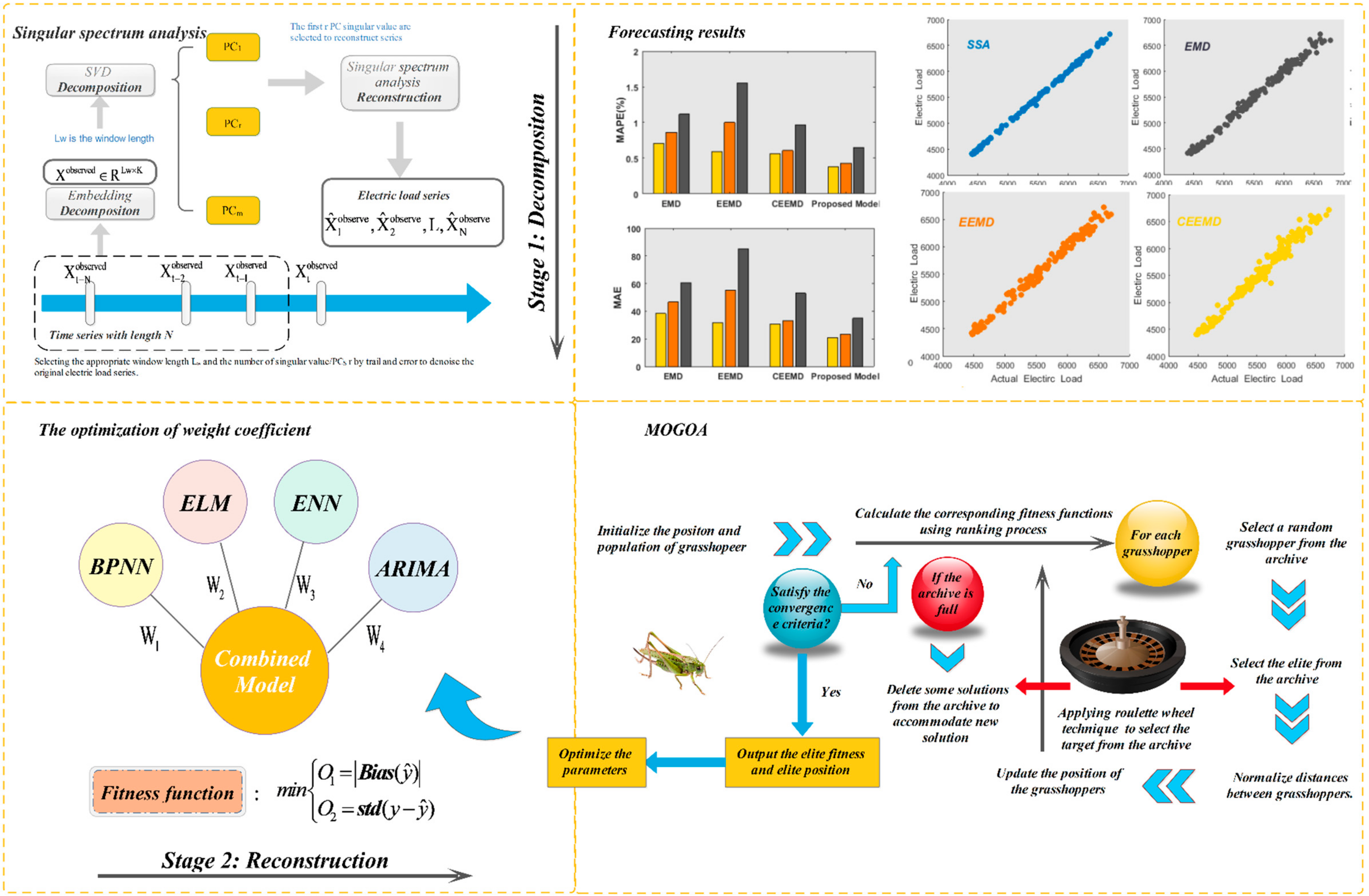
Applying the decomposition and reconstruction strategy, data preprocessing methods are adopted to extract main features of the original data by eliminating high-frequency signals, making predictions more accurate. Decomposing the original power data and reconstructing it into a filtering sequence can eliminate the irregularity and uncertainty of the data and achieve better power load forecasting performance.

(2)

Applying the multiobjective optimization algorithm, the optimal weight coefficient of each single model can be optimized. Our proposed combined model is not only robust, but also economical in power load forecasting. Moreover, it has higher precision and greater stability.

(3)

With the combination of the linear model (ARIMA) and nonlinear models (WNN, ELM, and BPNN), the developed model can reflect both the linearity and nonlinearity of electrical load data. Our proposed model can use each individual model thoroughly and it spontaneously overcomes limitations such as low precision and instability to ensure the effectiveness of power load forecasting.

(4)

The new combined model beats other single models and will provide effective technical support for power system management. The developed model was simulated and examined based on the electric load data of three different sites, which indicates its strong robustness and adaptability regardless of location and forecasting steps.

The rest of the paper is arranged as follows. In Section 2, we introduce the methodology we applied in the proposed model, including the data preprocessing technique, ARIMA, WNN, ELM, BPNN, the theory of combined models, and multiobjective grasshopper optimization. Section 3 describes the electric load time series we selected and three experiments aimed at verifying the effectiveness of our forecasting model. In Section 4, we provide an in-depth discussion of the proposed model, including a test of the performance of the proposed optimization algorithm, two tests of the effectiveness of the model, and a test showing the improvement of the model and a comparative experiment of the combination method.

3. Methods

In this section, we discuss the methods of the proposed combined model in detail, including the singular spectrum analysis (SSA) technique, the individual models used in the combined model, and the multiobjective grasshopper optimization algorithm (MOGOA). After that, a combined model that can significantly improve the definition of electric load forecasting is presented.

3.1. SSA Technique

SSA is a nonparametric spectral estimation method usually used for filtering in the preprocessing stage of time series forecasting. The advantage of SSA is that it always works well in both linear and nonlinear time series. Moreover, it performs well whether the time series is stationary or not. In short, the way SSA works is to identify the trend and noise parts of a time series, after which it reconstructs a new series.

3.2. Wavelet Neural Network

Wavelet neural network (WNN) is a modern artificial intelligence model. It is essentially a feed-forward neural network based on wavelet transform [53]. Its basic working principle is to use wavelet space as the feature space of pattern recognition to realize the feature extraction of signals by weighting the inner product of the wavelet base and the signal vector and combining the time-frequency localization of the wavelet transform and the self-learning function of the neural network. It has the advantage of being able to effectively learn the input/output characteristics of the system without the need for a priori information such as data structures and characteristics. In addition, compared with traditional neural networks, wavelet neural networks can often achieve better prediction accuracy, faster convergence, and better fault tolerance when forecasting in complex nonlinear, uncertain, and unknown systems. So, we applied WNN as an individual nonlinear model in our proposed model.

3.3. Extreme Learning Machine

Extreme learning machine (ELM) is a kind of machine learning algorithm based on feed-forward neuron network [54]. Its main feature is that the hidden layer node parameters can be given randomly or artificially and do not need to be adjusted. The learning process only needs to calculate the output weight. ELM has the advantages of high learning efficiency and strong generalization ability and is widely used in time series forecasting. As a result, we applied ELM as an individual nonlinear model in our proposed model.

3.4. Back Propagation Neural Network

The back propagation neural network (BPNN), composed of an input layer, a hidden layer, and an output layer, is a concept that was proposed by scientists led by Rumelhart and McClelland in 1986 [55]. It is a multilayer feed-forward neural network trained according to the error back propagation algorithm. Learning and working stages are the whole process of BPNN. It is the most widely used neural network. It has arbitrary complex pattern classification ability and excellent multidimensional function mapping ability, which solves the exclusive OR (XOR) and other problems that cannot be solved by simple perception. In essence, the BP algorithm uses the network error squared as the objective function and the gradient descent method to calculate the minimum value of the objective function. Moreover, because of its flexible structure and strong nonlinear mapping capability, BPNN is widely applied in the engineering field. So, we applied it as an individual nonlinear model in our proposed model.

3.5. Autoregressive Integrated Moving Average Model

The ARIMA model, also known as the autoregressive moving average model, is a model used for time series forecasting with relatively high prediction accuracy. The ARIMA model mainly consists of 3 forms, a moving average MA model, an autoregressive AR model, and a mixture of autoregressive moving average ARMA models. Before using this model, it is necessary to first analyze whether the time series is stable. If the sequence is a nonstationary time series, the first step is to differentiate the time series, and the difference must be smoothed before the model is established, otherwise it cannot be used.

The difference between the ARIMA model and the ARMA model is that the ARMA model is built for stationary time series and the ARIMA model is used for nonstationary time series. In other words, to establish an ARMA model for a nonstationary time series, you first need to transform into a stationary time series and then build an ARMA model. We applied ARIMA as an individual linear model in our proposed model.

3.6. Basic concepts of Multiobjective Optimization Problems

Conventional relational operators such as >, <, and =, which are always found in single-objective optimization problems, cannot be applied in multiobjective optimization. To address this problem, a new concept of dominates was proposed and then extended by Edgeworth in 1881 and Pareto in 1964. Details of Pareto dominance are as follows:

Definition 1 (Pareto dominance):

The definition of Pareto dominance is: vector $y=\left(y_1,y_{2,\dots }{y}_z\right)$ is dominated by vector $x=\left(x_1,x_{2,\dots }{x}_z\right)$ (i.e., x > y) when

$$\forall t\in \left[1,z\right],\left[f(x_t)\ge f(y_t)\right]\wedge \left[\exists t\in [1,z]:f(x_t)>f(y_t)\right]$$

(1)

where z represents the length of vectors.

3.7. Multiobjective Grasshopper Optimization Algorithm

MOGOA is the latest nature-inspired method, proposed by Mirjalili [56]. Essentially, MOGOA is a multiobjective version of GOA. GOA is a nature-inspired algorithm that simulates the swarming behavior of grasshoppers. The position of a grasshopper in the swarm representing a possible solution of a given single-objective optimization problem is the main principal of GOA. The details of MOGOA, and the main steps of building it, are as follows:

In order to replicate the real living conditions of grasshoppers in nature, MOGOA takes 3 factors—gravity force, social interaction, and wind advection—into the model. $X_i$ means the position of the ith grasshopper and is represented by:

$$X_i=S_i+G_i+A_i$$

(2)

where $S_i$, $G_i$, and $A_i$ mean social interaction, gravity force, and wind advection, respectively.

Social interaction is the most important factor, calculated by the following equation:

$$S_i={\displaystyle \sum _{\begin{array}{l}j=1\\ j\ne i\end{array}}^{N}s(d_{ij})}{\widehat{d}}_{ij}$$

(3)

$$d_{ij}=\left|x_j-x_i\right|$$

(4)

$${\widehat{d}}_{ij}=\left(x_j-x_i\right)/d_{ij}$$

(5)

$$s(r)=f{e}^{-r/l}-e^{-r}$$

(6)

where $d_{ij}$ means the distance between the ith and jth grasshoppers, and ${\widehat{d}}_{ij}$ is a unit vector of $d_{ij}$. Function s defines that the values of parameters f and l are changed, so the social forces can be changed too. The distance between grasshoppers is limited to the interval of [1,4], because, according to common sense, when 2 grasshoppers are far apart, they will not have a strong social influence on each other. Gravity force is defined as:

$$G_i=-g{\widehat{e}}_g$$

(7)

where g is the gravitational constant and ${\widehat{e}}_g$ represents the unity vector toward the center of the earth. Wind advection is defined as:

$$A_i=u{\widehat{e}}_w$$

(8)

where u means constant drift and ${\widehat{e}}_w$ represents the unity vector in the wind direction. After replacing Equation (2) with the above 3 equations, we can get:

$$X_i={\displaystyle \sum _{\begin{array}{l}j=1\\ j\ne i\end{array}}^{N}s(\left|x_j-x_i\right|)\frac{x_j-x_i}{d_{ij}}-g{\widehat{e}}_g+u{\widehat{e}}_w}$$

(9)

Considering that the influence of gravity force on grasshoppers is too weak and assuming that the wind direction is always toward the best solution ${\hat{\mathit{T}}}_d$, some parameters are added to the mathematical model to enhance the ability to explore and exploit for the purpose of solving the optimization problem more effectively. After that, the mathematical model turns to:

$$X_i{}^d=c({\displaystyle \sum _{\begin{array}{l}j=1\\ j\ne i\end{array}}^{N}c\frac{u{b}_d-l{b}_d}{2}s(\left|x_j{}^d-x_i{}^d\right|)}\frac{x_j-x_i}{d_{ij}})+{\widehat{T}}_d$$

(10)

where $\mathit{u}{\mathit{b}}_d$ and $\mathit{l}{\mathit{b}}_d$ are the upper and lower bound of the dth dimension, respectively, and ${\hat{\mathit{T}}}_d$ is the best solution’s dth dimension value so far. For the purpose of reducing exploration and increasing exploitation proportional to $c_{\max }$ at the same time, the parameter $\mathit{c}$ is updated with the following equation:

$$c=c_{\max }-l\frac{c_{\max }-c_{\min }}{L}$$

(11)

Compared with finding solutions from a series of Pareto optimal solutions obtained by MOGOA, it is easier to find the best solution calculated so far in a single-objective search. Because the archive has all the Pareto optimal solutions, the position of the target is determined. Finding the target that can improve the solution’s distribution becomes the biggest problem. The possibility of choosing the target from the archive is calculated by:

$$P_i=\frac{1}{N_i}$$

(12)

where Ni represents the neighborhood of the ith solution’s total number. With this probability, there are 2 advantages to using the roulette method when selecting a target from a file: first, the roulette method can improve the distribution of less distributed areas of the search space, and second, when premature convergence occurs, a solution with a crowded neighborhood can be selected as a target to solve the problem.

When updating the content of the archive regularly in MOGOA, 2 criteria are implemented: (1) give up an external solution as long as this external solution is dominated by one archive solution; and (2) add an external solution to the archive when the external solution does not dominate all solutions inside the archive. Moreover, as long as an external solution dominates a solution inside the archive, the inside one should be replaced by the external one. All in all, MOGOA can not only find Pareto optimal solutions, but also store them in an archive.

The pseudocode of MOGOA is as follows:

Algorithm 1:MOGOA
	Objective functions: $$min\{\begin{array}{l}{O}_1=\left|\mathit{B}\mathit{i}\mathit{a}\mathit{s}(\widehat{y})\right|\\ O_2=\mathit{s}\mathit{t}\mathit{d}(y-\widehat{y})\end{array}$$ Input: ${\widehat{y}}_B=\left({\widehat{y}}_B(1),{\widehat{y}}_B(2),\cdots ,{\widehat{y}}_B(q)\right)$- BPNN ${\widehat{y}}_E=\left({\widehat{y}}_E(1),{\widehat{y}}_E(2),\cdots ,{\widehat{y}}_E(q)\right)$- ELM ${\widehat{y}}_W=\left({\widehat{y}}_W(1),{\widehat{y}}_W(2),\cdots ,{\widehat{y}}_W(q)\right)$-WNN ${\widehat{y}}_A=\left({\widehat{y}}_A\left(1\right),{\widehat{y}}_A\left(2\right),\cdots ,{\widehat{y}}_A\left(q\right)\right)$-ARIMA Output: ${\widehat{y}}_f=\left({\widehat{y}}_f(1),{\widehat{y}}_f(2),\cdots ,{\widehat{y}}_f(l)\right)$- forecasting results
	Parameters: L—the maximum number of iterations n—the number of grasshoppers [$\mathit{l}{\mathit{b}}_i$,$\mathit{u}{\mathit{b}}_i$] —boundaries of the i-th variable xi—i-th grasshopper’s position l—current iteration number d—dimension amount. ${\mathit{c}}_{\max }$—c’s maximum value ${\mathit{c}}_{\min }$— c’s minimum value ${\hat{\mathit{T}}}_d$—best solution’s d-th dimension value so far dij—the distance between the i-th and the j-th grasshopper s—social forces function

3.8. SSA-MOGOA Combined Model

In our study, a new combined model applying a data preprocessing technique, a new parameter determination method, and several individual prediction algorithms, including both linear and nonlinear models, is successfully developed. The main steps are listed below. The flowcharts of the proposed model are depicted in Figure 1.

3.8.1. Stage 1: Data Preprocessing

SSA is a nonparametric spectral estimation method usually used for filtering in the preprocessing stage of time series forecasting [57]. The advantage of SSA is that it always works well in both linear and nonlinear time series. In addition, the processed data will be used in subsequent forecasting. The main steps of SSA are depicted in Figure 1.

3.8.2. Stage 2: Individual Models used for Forecasting

Three nonlinear models, BPNN, ELM, and WNN, and a linear model, ARIMA, are chosen as the individual models that together form the combined model. It is worth mentioning that all 4 models can achieve good prediction results in our electric load forecasting.

3.8.3. Stage 3: Optimization of Weight Parameters of Combined Model

Determining the parameter coefficients of each individual model is very important for construction of the combined model. In past combined models, a simple average coefficient allocation strategy was often used. In our research, we adopted a multiobjective optimization algorithm called MOGOA for the deciding parameters and made the combined model achieve good prediction results in electric load forecasting.

4. Experiments and Analysis

In this section, we introduce the electric load time series we selected and the performance metric and testing methods. We also present three experiments aimed at verifying the effectiveness of our forecasting model. The main steps and flowchart of the developed model are described in Figure 1, which includes a data preprocessing technique, application of several individual models, optimization of the combined model’s weight coefficients, and forecasting results.

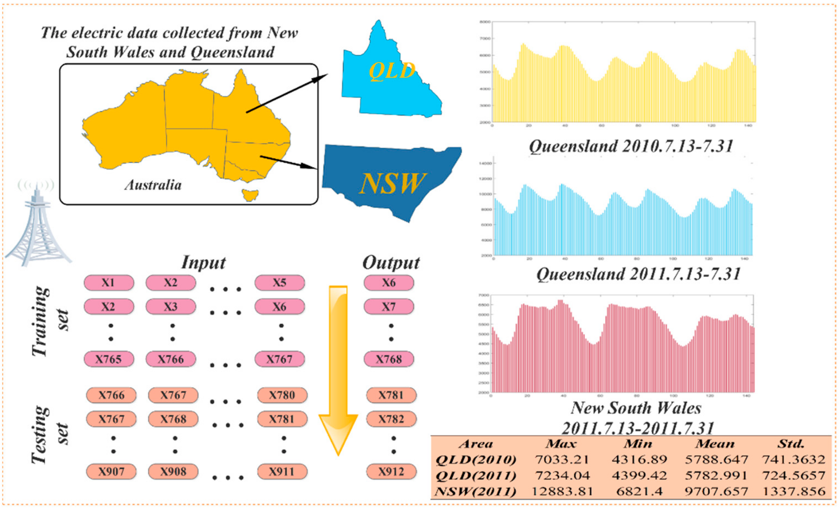
4.1. Datasets

In this paper, original electric load time series data were collected from two areas in Australia, New South Wales (NSW) and Queensland (QLD), on a half-hourly basis (48 data points per day). Two datasets were collected in New South Wales and Queensland, which were sampled from 13 to 31 July 2011, 19 days in all. The third dataset was sampled from 13 to 31 July 2010 in Queensland. Figure 2 presents a simple map of the study area, some descriptive statistical indicators of the datasets, and three general trends of testing samples. Specifically, in each dataset, the training set included 768 data points and the testing set consisted of 144 data points. There were 48 data points in a single day according to the data, therefore we selected the period T = 48 for the combined model. Statistical indicators including minimum, maximum, mean, and standard deviation are listed in

Table 1. Statistical indicators of experimental samples for three sites.

Dataset.	Samples	Numbers	Statistical Indicator(kw)
			Max	Min	Mean	Std.
QLD(2010)	All samples	912	7033.21	4316.89	5788.65	741.36
	Training	768	7033.21	4316.89	5803.04	746.40
	Testing	144	6476.49	4361.6	5711.87	708.99
QLD(2011)	All samples	912	7234.04	4399.42	5782.99	724.57
	Training	768	7234.04	4412.33	5834.35	729.96
	Testing	144	6718.05	4399.42	5509.06	627.75
NSW(2011)	All samples	912	12883.81	6821.4	9707.66	1337.86
	Training	768	12883.81	6821.4	9819.03	1346.71
	Testing	144	11314.46	6939.18	9113.68	1115.41

. From one-step to three-step prediction, forecasting outcomes are all based on the historical data, which means this experimental outcome is not used as input data to forecast the subsequent values in this study, while in artificial intelligence models, based on plenty of experimental results, five historical data points are chosen as input so as to obtain the best forecasting performance in the multistep forecasting mechanism. The detailed data structure is presented in Figure 2.

4.2. Performance Metrics

In our study, to evaluate the predictive power of the proposed model, we needed performance metrics in our time forecasting experiments. Because there is no general standard for evaluating a time forecasting model, we decided to apply three performance metrics: mean absolute error (MAE), root mean square error (RMSE), and mean absolute percent error (MAPE), as presented in

Table 2. Three error metrics.

Metric	Definition	Equation
MAE	The mean absolute error of N forecasting results	$\mathrm{MAE}=\frac{1}{N}{\displaystyle \sum _{i=1}^N\left|F_i-A_i\right|}$
RMSE	The square root of the average of error squares	$\mathrm{RMSE}=\sqrt{\frac{1}{N}\times {\displaystyle \sum _{i=1}^N{\left(F_i-A_i\right)}^2}}$
MAPE	The average of N absolute percentage error	$\mathrm{MAPE}=\frac{1}{N}{\displaystyle \sum _{i=1}^N\left|\frac{A_i-F_i}{A_i}\right|}\times 100\%$

[58]. Next, we introduce these three performance metrics in detail.

From the definitions of MAE and RMSE, it is obvious that the advantage of these two performance metrics is that they can avoid canceling between positive and negative forecasting errors due to the use of absolute value symbols. They can evaluate the average dimension of the forecasted time series with actual data. MAPE, which is regarded as the most widely used performance metric in time series forecasting, is obtained by calculating the average of absolute error. The advantage of MAPE is that it can reflect the reliability and validity of the time series forecasting method. When observing the values of all three of these metrics, the smaller the value, the more accurate the prediction. Table 2 shows the formulas of the three error metrics. Here Ai means actual values of the time series and Fi means predicted values, and N means sample size.

4.3. Testing Method

In this section, we introduce the Diebold–Mariano (DM) test and the forecasting effectiveness that were applied to statistically test the accuracy of our proposed model in time series forecasting.

4.3.1. Diebold–Mariano Test

Diebold and Mariano [59] developed a test to compare a model’s prediction efficiency with that of other models. The main steps of the DM test are as follows:

Since the DM test is essentially a hypothesis test, the first things to introduce are the null hypothesis $H_0$ and alternative hypothesis $H_1$:

$$H_0:E\left[F\left(e_t^1\right)\right]=E\left[F\left(e_t^2\right)\right]$$

(13)

$$H_1:E\left[F\left(e_t^1\right)\right]\ne E\left[F\left(e_t^2\right)\right]$$

(14)

where $e_t^1$ and $e_t^2$ are subtracted from actual time series data and the different models’ predicted time series values, also called forecasting errors, and F is the loss function of $e_t^1$ and $e_t^2$.

$$\overline{d}=\frac{1}{L}{\displaystyle \sum _{t=1}^L\left[F\left(e_t^1\right)-F\left(e_t^2\right)\right]}$$

(15)

$\overline{d}$ is obtained by calculating the average of the sum of differences between the two models’ loss function, and L is the length of predicted values.

$$DM=\frac{\overline{d}}{\sqrt{2\pi \stackrel{\sim }{f_d\left(0\right)}/L}}\to N\left(0,1\right)$$

(16)

As shown in the above formula, the test statistic DM is convergent in the standard normal distribution N (0, 1). The null hypothesis will be rejected if $\left|DM\right|$ is bigger than $\left|Z_{\alpha /2}\right|$, where $z_{\alpha /2}$ stands for the critical z-value of the standard normal distribution and $\alpha$ denotes the significance level.

4.3.2. Forecasting Effectiveness

Forecasting effectiveness can be calculated by the accuracy of the mean squared deviation, which the DM test cannot do [60]. Forecasting effectiveness is also employed in our study. The principal ideas of forecasting effectiveness are as follows:

$m^k={\displaystyle \sum _{i=1}^n{Q}_i{A}_i^k}$ is used to calculate the kth order forecasting effectiveness unit, where Ai means forecasting accuracy time i; $Q_i$ object to ${\displaystyle \sum _{i=1}^n{Q}_i}=1, Q_i>0$, called discrete possibility distribution. $Q_i$ will be defined as $Q_i=1/n, i=1,2,\dots ,n$ when there is no prior information of $Q_i$. The kth order forecasting effectiveness is calculated by $H\left(m^1,m^2,\cdots ,m^k\right)$, where H is a continuous function with k units. The first-order forecasting effectiveness will be defined as $H\left(m^1\right)=m^1$ when $H(\mathrm{x})=x$ is a continuous constant function. $H\left(m^1,m^2\right)=m^1\left(1-\sqrt{m^2-{\left(m^1\right)}^2}\right)$ will be called as the second-order forecasting effectiveness when $H\left(x,y\right)=x\left(1-\sqrt{y-x^2}\right)$ is a continuous function with two variables.

4.4. Experiments and Analysis

In this part, to examine our proposed model’s performance in electric load time series forecasting, we did three experiments from corresponding power station sites.

4.4.1. Experiment I: Compare with Other Models Based on SSA

In order to determine the necessity of combining the models, we made this experiment comparing the electric load time series forecasting results of our new model with the four SSA-based models. The experimental results are shown in

Table 3. Comparison of proposed model with other SSA-based models.

Dataset	Model	MAE			RMSE			MAPE (%)
		1-step	2-step	3-step	1-step	2-step	3-step	1-step	2-step	3-step
QLD(2010)	SSA-BP	24.78	32.79	62.15	30.87	39.70	80.51	0.44	0.58	1.10
	SSA-ELM	22.35	36.58	68.08	28.35	44.18	86.52	0.40	0.66	1.20
	SSA-WNN	26.23	52.69	95.45	36.09	68.78	126.16	0.47	0.93	1.71
	SSA-ARIMA	39.18	40.71	43.54	52.83	54.84	57.59	0.70	0.72	0.78
	Proposed Model	21.26	25.94	37.97	26.98	32.83	46.51	0.37	0.45	0.68
QLD(2011)	SSA-BP	26.21	35.21	71.09	34.48	45.07	86.81	0.50	0.65	1.31
	SSA-ELM	23.90	34.98	90.62	30.43	45.20	118.89	0.44	0.65	1.69
	SSA-WNN	35.30	80.94	169.98	45.58	100.84	216.67	0.68	1.53	3.16
	SSA-ARIMA	42.82	44.60	48.70	58.27	58.10	61.19	0.77	0.81	0.90
	Proposed Model	20.79	23.43	34.84	27.75	30.73	44.80	0.38	0.43	0.65
NSW(2011)	SSA-BP	47.49	77.03	130.75	62.67	97.79	159.54	0.53	0.86	1.49
	SSA-ELM	46.43	73.69	153.61	59.45	90.02	197.51	0.51	0.82	1.74
	SSA-WNN	58.74	125.89	258.21	75.26	163.72	324.61	0.66	1.43	2.94
	SSA-ARIMA	90.62	95.95	105.31	127.67	128.47	130.37	0.99	1.04	1.16
	Proposed Model	44.29	57.83	77.74	57.63	73.87	97.92	0.48	0.64	0.86

. Detailed descriptions are as follows:

• By observing the experimental results using the 2010 Queensland power data, the following results were found: First of all, the most obvious was that our proposed combined model had the best prediction performance whether the statistical indicator was MAE, RMSE, or MAPE; in other words, the smallest error metrics values. Second, if we look closely at the forecasting steps, we can find that the forecasting accuracy gets worse. In one-step forecasting, our proposed model’s MAPE value is 0.37%, and it increases to 0.68% in three-step forecasting.
• For the 2011 Queensland power data, we found the following: First, our proposed model was still the most accurate one. It is worth mentioning that in one-step forecasting, the forecasting gap between our model and the SSA-ELM model was big. Specifically, the MAE values of our model and SSA-ELM were 20.79 and 23.90, respectively, while they were 21.26 and 22.35 with the 2011 Queensland power station data. The superiority of the proposed model can be more intuitively reflected in the Figure 3.
• Regarding the results using the 2011 New South Wales power data, compared to the first two experiments, which used electric load data from Queensland, the error metric values were significantly larger in the third experiment. This reflects the differences among different power plants. The great thing was that our proposed combined model still outperformed other SSA-based models in one-step to three-step forecasting. This is powerful proof that our model is indeed superior. At the same time, we can also determine the necessity of combining models through this experiment by the fact that it really can improve forecast accuracy.

N.B. By comparing the forecasting results of our proposed combined model with other SSA-based models, there were many useful findings from Experiment I. Our model’s overall performance in predicting accuracy demonstrates the need to combine models. Moreover, our proposed model greatly improves electric load forecasting accuracy with an average MAPE of 0.52% in all experiments.

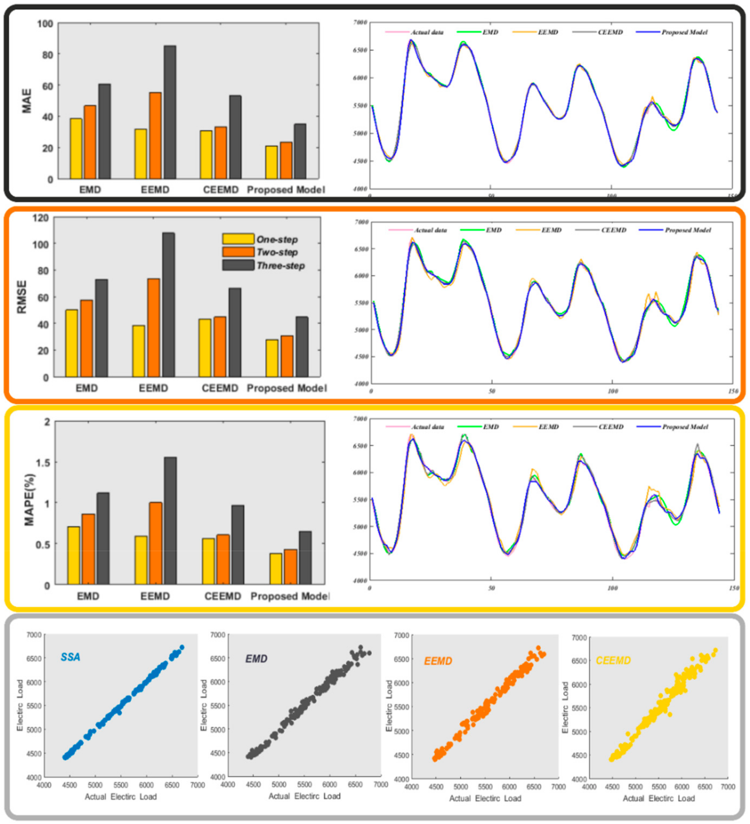
4.4.2. Experiment II: Comparing Models using Other Data Preprocessing Methods

In order to verify whether singular spectrum analysis (SSA) is the best choice for data processing, we conducted an experiment comparing the electric load time series forecasting results of our proposed model with other data processing method–based models. The experimental results are shown in

Table 4. Comparison of forecasting performance of combined model and models using different data preprocessing methods.

Dataset	Model	MAE			RMSE			MAPE (%)
		1-step	2-step	3-step	1-step	2-step	3-step	1-step	2-step	3-step
QLD(2010)	EMD	39.86	47.91	56.38	45.93	56.44	67.71	0.72	0.88	1.05
	EEMD	33.72	42.97	55.97	50.84	56.95	70.47	0.60	0.78	0.99
	CEEMD	30.04	35.90	51.47	36.74	44.14	64.19	0.54	0.64	0.90
	Proposed Model	21.26	25.94	37.97	26.98	32.83	46.51	0.37	0.45	0.68
QLD(2011)	EMD	38.37	46.63	60.59	50.13	57.51	72.93	0.71	0.86	1.12
	EEMD	31.56	55.11	84.83	38.57	73.23	107.65	0.59	1.00	1.56
	CEEMD	30.48	32.89	53.04	43.11	44.62	66.12	0.56	0.61	0.97
	Proposed Model	20.79	23.43	34.84	27.75	30.73	44.80	0.38	0.43	0.65
NSW(2011)	EMD	60.95	74.46	110.60	83.78	95.41	135.10	0.66	0.82	1.24
	EEMD	65.29	112.21	166.16	80.19	140.71	213.64	0.73	1.25	1.81
	CEEMD	62.29	82.48	100.39	82.51	100.77	125.26	0.67	0.92	1.12
	Proposed Model	44.29	57.83	77.74	57.63	73.87	97.92	0.48	0.64	0.86

. Detailed descriptions are as follows:

• Observing the experimental results using the 2010 Queensland power data, the proposed combined model achieved the highest forecasting accuracy. In contrast, the CEEMD preprocessed model was the most effective among the other three data processing methods, with MAPE values of 0.54%, 0.64%, and 0.90% from one-step to three-step forecasting, respectively. For the proposed model, MAPE values were 0.37%, 0.45%, and 0.68% from one to three steps, respectively.
• For the experiment using the 2011 Queensland power data, according to the evaluation criteria, the proposed model outperformed the other models. The MAPE values of the models using EMD, EEMD, and CEEMD were, respectively, 0.33%, 0.21%, and 0.18% higher than those of the proposed model in one-step forecasting. Figure 4 shows a comparison of the one- to three-step forecasting performance of Experiment II. It can be concluded that the proposed combined model achieved the highest accuracy compared to the models using other data preprocessing methods in three-step forecasting.
• When using the 2011 New South Wales power data, similar to Experiment I, compared to the first two experiments using data from Queensland, the error metric values of the third experiment were significantly larger. This reflects the difference between different power plants. In addition, there were also some interesting conclusions. For example, in the first two sets of power plant data, the CEEMD model performed better than the EMD model, but in the third group, the EMD and CEEMD models performed almost the same. However, our model still the performed the best. We can also determine the necessity of applying singular spectrum analysis (SSA) in our model so that it performs better than the other three classic data processing methods.

N.B. In experiment II, by comparing the forecasting results of our proposed combined model with other models using different data processing methods, there are many useful findings. Our model’s overall lead in predicting accuracy demonstrates that SSA is the best choice of data processing method.

4.4.3. Experiment III: Comparing with Classic Models

In Experiment III we took the forecasting results of our proposed model and the artificial intelligence model to compare the BP, WNN, ELM, and ARIMA. In order to make the experiment more complete and persuasive, we also compared it with some classic conventional models. The experimental results are shown in

Table 5. Comparison of forecasting performance of combined model and some classic individual models.

Dataset	Model	MAE			RMSE			MAPE (%)
		1-step	2-step	3-step	1-step	2-step	3-step	1-step	2-step	3-step
QLD(2010)	BP	46.12	80.44	119.79	59.34	102.45	150.21	0.81	1.40	2.10
	BP-MODA	47.54	86.23	121.67	59.98	108.89	162.77	0.84	1.52	2.13
	WNN	51.24	99.72	145.12	64.72	136.56	189.77	0.90	1.75	2.58
	ENN	45.76	82.88	126.34	60.95	104.71	168.20	0.80	1.46	2.24
	ELM	46.24	85.19	130.82	59.28	110.41	171.58	0.81	1.50	2.34
	RBF	64.08	134.02	185.37	86.13	185.85	275.07	1.12	2.33	3.22
	ARIMA	38.97	73.96	88.00	49.44	91.95	105.91	0.70	1.32	1.58
	Proposed Model	21.26	25.94	37.97	26.98	32.83	46.51	0.37	0.45	0.68
QLD(2011)	BP	45.61	93.75	147.05	64.12	127.47	217.66	0.82	1.71	2.66
	BP-MODA	44.23	85.21	124.31	61.31	116.22	163.60	0.79	1.56	2.28
	WNN	62.72	138.62	200.49	80.68	181.26	268.88	1.16	2.55	3.75
	ENN	50.62	98.11	152.69	70.11	135.34	207.65	0.92	1.80	2.79
	ELM	48.77	96.45	158.82	66.91	133.68	216.32	0.89	1.76	2.91
	RBF	85.22	170.73	308.71	198.05	524.76	971.50	1.53	3.10	5.64
	ARIMA	37.50	68.01	87.55	46.94	87.81	107.32	0.71	1.28	1.64
	Proposed Model	20.79	23.43	34.84	27.75	30.73	44.80	0.38	0.43	0.65
NSW(2011)	BP	89.72	163.56	276.83	124.34	215.84	349.76	0.96	1.79	3.05
	BP-MODA	85.23	180.48	268.43	110.79	251.79	360.47	0.92	1.98	2.94
	WNN	92.97	243.25	400.39	118.54	323.58	538.95	1.02	2.71	4.52
	ENN	101.07	191.08	282.89	133.22	265.73	362.33	1.09	2.08	3.13
	ELM	98.76	205.09	317.34	130.92	274.27	410.74	1.06	2.24	3.53
	RBF	149.92	216.50	351.10	280.01	318.79	449.90	1.60	2.36	3.84
	ARIMA	78.00	130.15	159.76	95.68	161.82	203.99	0.88	1.46	1.80
	Proposed Model	44.29	57.83	77.74	57.63	73.87	97.92	0.48	0.64	0.86

. Figure 5 shows a comparison of the one- to three-step forecasting performance of Experiment III. Detailed descriptions are as follows:

• With the experiments using the 2010 Queensland power data, we found that, first, our proposed combined model had the best prediction performance whether the statistical indicator was MAE, RMSE, or MAPE. For instance, taking the one-step forecasting MAE values for comparison, the values were 46.12, 47.54, 51.24, 45.76, 46.24, 64.08, 38.971, and 21.26. The proposed model’s MAE value was only about half of other methods’ values. Second, in two- and three-step forecasting, the combined model was more effective than the other methods. The prediction performance of all other models was significantly worse than that of our model and there was still a big gap, which was sufficient to reflect the excellence of our model.
• With the 2011 Queensland power data, the results were as follows: First, our proposed model was still the most accurate. Second, although the data were from a different year, it is clear that forecasting results of the first two experiments are fairly similar, which reflects the stability of our method. The RMSE values of the proposed model were 27.75, 30.73, and 44.80 for one to three steps, respectively.
• For the 2011 New South Wales power data, the RMSE values of the proposed model were 57.63, 73.87, and 97.92 for one to three steps, respectively. The great thing is that our proposed combined model still outperformed the other data processing methods in one- to three-step forecasting. This is powerful proof that our model is indeed the best of all eight models. Although not as accurate as the predictions in the first two experiments, the degree of improvement in the prediction results did not change much at around 50%. This will be discussed in the next section.

N.B. In experiment III, by observing the results including our proposed method, models that we applied in our model, and traditional models we did not use, we found that our model had an overall lead in predicting accuracy. This demonstrates that our proposed combined model will save a lot of energy for power systems and should be applied in actual electric load forecasting practice.

5. Discussion

This section provides an in-depth discussion of the proposed model, including a proposed optimization algorithm performance test, two proposed model effectiveness tests, and an experiment showing the improvements of the proposed model and a comparative experiment.

5.1. Multiobjective Grasshopper Algorithm Experiments

Four typical test functions (shown in

Table 6. Test functions of algorithms.

ZDT1	ZDT2
Minimize: $f_1(x)=x_1$ Minimize: $f_2(x)=g(x)\times h(f_1(x), g(x))$ Where: $g(x)=1+\frac{9}{N-1}{\displaystyle {\sum }_{i=2}^N{x}_i}$ $\begin{array}{l}h(f_1(x), g(x))=1-\sqrt{\frac{f_1(x)}{g(x)}}\\ 0\le x_1\le 1, 1\le i\le 30\end{array}$	Minimize: $f_1(x)=x_1$ Minimize: $f_2(x)=g(x)\times h(f_1(x), g(x))$ Where: $g(x)=1+\frac{9}{N-1}{\displaystyle {\sum }_{i=2}^N{x}_i}$ $h(f_1(x), g(x))=1-{\left(\frac{f_1(x)}{g(x)}\right)}^2$ $0\le x_1\le 1, 1\le i\le 30$
ZDT3	ZDT1 with linear front
Minimize: $f_1(x)=x_1$ Minimize: $f_2(x)=g(x)\times h(f_1(x), g(x))$ Where: $g(x)=1+\frac{9}{N-1}{\displaystyle {\sum }_{i=2}^N{x}_i}$ $\begin{array}{l}h(f_1(x), g(x))=1-\sqrt{\frac{f_1(x)}{g(x)}}\\ -\left(\frac{f_1(x)}{g(x)}\right)\sin (10\pi f_1(x))\\ 0\le x_1\le 1, 1\le i\le 30\end{array}$	Minimize: $f_1(x)=x_1$ Minimize: $f_2(x)=g(x)\times h(f_1(x), g(x))$ Where: $g(x)=1+\frac{9}{N-1}{\displaystyle {\sum }_{i=2}^N{x}_i}$ $\begin{array}{l}h(f_1(x), g(x))=1-\frac{f_1(x)}{g(x)}\\ 0\le x_1\le 1, 1\le i\le 30\end{array}$

) were applied to examine the excellence of the proposed algorithm. We chose multiobjective ant lion optimization (MOALO) and the multiobjective dragonfly algorithm (MODA) to compare with MOGOA to examine its optimization performance. To control variables, we set the maximum iterations and search agents as 100 and the size of archive as 150. We applied inverted generational distance (IGD), which is a metric showing the evaluation degree of multiobjective optimization algorithms.

Table 7. Results of multiobjective algorithms using inverted generational distance (IGD) on four test functions.

Algorithm	Ave.	Std.	Median	Min	Max
ZDT1
MOALO	0.006213	0.007038	0.005901	0.004272	0.024323
MODA	0.005826	0.005798	0.005082	0.002613	0.025404
MOGOA	0.004275	0.003089	0.004669	0.002573	0.024234
ZDT2
MOALO	0.009454	0.007343	0.008998	0.004738	0.022138
MODA	0.008173	0.005193	0.008532	0.003643	0.023234
MOGOA	0.008015	0.003140	0.005395	0.002157	0.023118
ZDT3
MOALO	0.027063	0.000867	0.026627	0.028135	0.026727
MODA	0.025089	0.000521	0.024982	0.028182	0.027322
MOGOA	0.024270	0.000469	0.024246	0.024186	0.023801
ZDT1 with linear front
MOALO	0.006821	0.005623	0.006532	0.005431	0.026626
MODA	0.006101	0.005541	0.005926	0.003863	0.024777
MOGOA	0.005569	0.004986	0.003985	0.002211	0.024461

shows the test results of IGD, for which we did 60 experiments for every test function [61]. Moreover, Figure 6 shows the obtained Pareto optimal solutions by these three algorithms.

From the experimental results we can see the following:

(a)

MOGOA gets the best IGD values among the optimization algorithms in all four test functions, which proves that its optimizing ability is superior to that of MODA and MOALO.

(b)

By observing the contrast of the number of the Pareto optimal solutions calculated by MOGOA, MODA, and MOALO shown in Figure 6, we find that MOGOA had the most Pareto optimal solutions among all three algorithms.

N.B. The optimization ability of MOGOA is proven to be good through the experiment and discussion above. Therefore, MOGOA can be widely applied to deal with multiobjective optimization problems.

5.2. Proposed Model’s Effectiveness

The Diebold–Mariano test was used to verify the validity of the developed model, which means every model mentioned above was compared to the SSA-MOGOA combined model. The DM test is a kind of hypothetical test. The null hypothesis is that there is no significant difference in the models’ forecasting performance. The opposite hypothesis is that there is a significant different in the models’ forecasting performance.

Table 8. DM test of different models.

Model	1-step	2-step	3-step
SSA-BP	2.7503 *	3.8971 *	6.1244 *
SSA-ELM	1.6379 **	3.9104 *	6.3244 *
SSA-WNN	4.0126 *	6.8486 *	7.3544 *
SSA-ARIMA	4.9261 *	5.0164 *	4.0033 *
EMD	5.4365 *	5.5545 *	5.7057 *
EEMD	4.3034 *	5.0669 *	5.21 *
CEEMD	3.7225 *	3.8063 *	4.3806 *
BP	4.7348 *	5.9805 *	6.3855 *
BP-MODA	5.2960 *	5.8782 *	6.2118 *
WNN	6.3481 *	6.2092 *	7.1581 *
ENN	5.3966 *	6.1685 *	6.3538 *
ELM	5.4820 *	5.7369 *	6.3290 *
RBF	3.3792 *	3.7372 *	3.5957 *
ARIMA	5.6641 *	7.0336 *	7.5187 *

* 1% significance level; ** 5% significance level.

shows average DM test values of all experiments for one- to three-step forecasting.

Table 8 shows that except for the one-step SSA-ELM experiment, the DM value in all the other experiments is big enough to be rejected at the 1% significance level, while the null hypothesis of one-step SSA-ELM is rejected at 5%. Moreover, for the DM test of individual models, the value is 3.3792, which shows that the accuracy of the proposed model is fairly high.

To further evaluate our model, as introduced in Section 3.3, we also applied the forecasting effectiveness method in our testing experiments. Forecasting effectiveness can effectively reflect the accuracy of the forecasting performance of various models, making it easy to comparing their pros and cons. In

Table 9. Forecasting effectiveness of different models.

Model	1-step		2-step		3-step
	1-order	2-order	1-order	2-order	1-order	2-order
Proposed Model	0.9959	0.9962	0.9949	0.9957	0.9927	0.9935
SSA-BP	0.9951	0.9950	0.9931	0.9935	0.9870	0.9869
SSA-ELM	0.9955	0.9956	0.9929	0.9935	0.9846	0.9831
SSA-WNN	0.9940	0.9932	0.9870	0.9847	0.9740	0.9684
SSA-ARIMA	0.9918	0.9923	0.9914	0.9919	0.9905	0.9910
EMD	0.9930	0.9929	0.9915	0.9914	0.9887	0.9888
EEMD	0.9936	0.9941	0.9899	0.9900	0.9855	0.9844
CEEMD	0.9941	0.9944	0.9928	0.9939	0.9900	0.9903
BP	0.9914	0.9918	0.9837	0.9829	0.9740	0.9734
BP-MODA	0.9915	0.9921	0.9831	0.9844	0.9755	0.9772
WNN	0.9897	0.9884	0.9766	0.9745	0.9638	0.9625
ENN	0.9906	0.9908	0.9822	0.9820	0.9728	0.9721
ELM	0.9908	0.9911	0.9817	0.9824	0.9707	0.9709
RBF	0.9858	0.9847	0.9740	0.9690	0.9589	0.9473
ARIMA	0.9924	0.9929	0.9865	0.9872	0.9833	0.9836

, we record the detailed forecasting effectiveness values of all models in one- to three-step forecasting.

The forecasting effectiveness results in Table 9 show the following results: First, the most obvious is that our proposed combined model has the best prediction performance with the highest forecasting effectiveness values in all forecasting. Second, the prediction performance of other individual models is significantly worse than that of our model and there is still a big gap between them and our proposed model, which is sufficient to reflect the excellence of our model.

5.3. Proposed Combined Model’s Improvements

In order to make the traditional MAPE criteria more clear in comparing the pros and cons of the models, in this paper we propose a new form of MAPE, defined as:

$$P_{MAPE}=\left|\frac{MAP{E}_1-MAP{E}_2}{MAP{E}_1}\right|$$

(17)

This new MAPE criterion is used to compare the proposed model with the other models in the above experiments, including three data denoising algorithms, seven classic models, and four individual models with singular spectrum analysis.

Table 10. Percentage improvement of the proposed model.

Model	Site 1			Site 2			Site 3			Average
	1-step	2-step	3-step	1-step	2-step	3-step	1-step	2-step	3-step	1-step	2-step	3-step
SSA-BP	22.64%	33.80%	50.34%	8.66%	25.58%	42.01%	14.66%	21.23%	38.48%	15.32%	26.87%	43.61%
SSA-ELM	12.61%	33.77%	61.43%	4.96%	22.46%	50.35%	5.55%	31.32%	43.85%	7.71%	29.18%	51.88%
SSA-WNN	43.95%	71.78%	79.41%	27.19%	55.24%	70.63%	19.65%	51.45%	60.49%	30.26%	59.49%	70.18%
SSA-ARIMA	50.37%	46.41%	27.33%	51.26%	38.70%	25.26%	46.33%	37.50%	13.76%	49.32%	40.87%	22.12%
EMD	45.58%	49.99%	41.74%	27.16%	22.09%	30.29%	48.34%	48.42%	35.46%	40.36%	40.17%	35.83%
EEMD	35.39%	56.84%	58.19%	34.38%	48.75%	52.29%	37.92%	41.76%	32.02%	35.90%	49.12%	47.50%
CEEMD	31.79%	28.77%	32.63%	28.47%	30.30%	23.02%	30.47%	29.66%	25.22%	30.24%	29.58%	26.96%
BP	53.29%	74.77%	75.57%	49.74%	64.28%	71.63%	53.78%	67.55%	67.77%	52.27%	68.87%	71.66%
BP-MODA	51.66%	72.40%	71.48%	47.87%	67.72%	70.57%	55.26%	70.17%	68.35%	51.60%	70.10%	70.13%
WNN	66.78%	83.08%	82.65%	52.83%	76.47%	80.86%	58.62%	74.15%	73.79%	59.41%	77.90%	79.10%
ENN	58.38%	76.02%	76.67%	55.70%	69.29%	72.41%	53.43%	68.92%	69.90%	55.84%	71.41%	72.99%
ELM	56.65%	75.48%	77.67%	54.65%	71.56%	75.49%	53.92%	69.74%	71.14%	55.07%	72.26%	74.77%
RBF	74.90%	86.07%	88.46%	69.96%	72.97%	77.51%	66.48%	80.54%	79.01%	70.45%	79.86%	81.66%
ARIMA	45.65%	66.20%	60.38%	45.25%	56.24%	51.93%	46.34%	65.59%	57.11%	45.75%	62.68%	56.47%

shows the experimental results, and some interesting conclusions can be summarized as follows:

• Comparing the proposed model with other SSA-based models, it is obvious that the novel proposed model has lower MAPE values. For example, the average improvement of the proposed model’s MAPE is 7.71%, 29.18%, and 51.88% compared with the SSA-ELM model, which is the least improved of the four models.
• Comparing the proposed model with the other three data preprocessing methods, its superiority is obvious. The lowest MAPE improvement is 22.09%, while the largest comes to 56.84%, which fully reflects the excellent prediction accuracy of our proposed model.
• Comparing the proposed model with the classic models, forecasting accuracy is greatly improved in every experiment. Compared with the ARIMA model, the proposed model improves by 45.75%, 62.68%, and 56.47% while the ARIMA model was the single model with the best prediction accuracy in the experiment.

5.4. Combined Strategy

We selected and applied a simple averaging strategy to calculate the prediction results of all individual models to compare with the results of MOGOA optimization to test the effectiveness of the proposed combination strategy. The results of the comparison between the two methods are shown in

Table 11. Comparison between proposed model and simple average strategy.

Dateset	Multi-Step	Model	MAE	RMSE	MAPE (%)
QLD(2010)	1-step	Simple average strategy	28.13	37.04	0.50
		Proposed model	21.26	26.98	0.37
	2-step	Simple average strategy	40.69	51.88	0.72
		Proposed model	25.94	32.83	0.45
	3-step	Simple average strategy	67.30	87.69	1.20
		Proposed model	37.97	46.51	0.68
QLD(2011)	1-step	Simple average strategy	32.06	42.19	0.60
		Proposed model	20.79	27.75	0.38
	2-step	Simple average strategy	48.93	62.31	0.91
		Proposed model	23.43	30.73	0.43
	3-step	Simple average strategy	95.10	120.89	1.76
		Proposed model	34.84	44.80	0.65
NSW(2011)	1-step	Simple average strategy	60.82	81.26	0.67
		Proposed model	44.29	57.63	0.48
	2-step	Simple average strategy	93.14	120.00	1.04
		Proposed model	57.83	73.87	0.64
	3-step	Simple average strategy	161.97	203.01	1.83
		Proposed model	77.74	97.92	0.86

.

From Table 11, we can easily find from the prediction results that the proposed combined model using MOGOA always outperformed the model applying a simple average strategy, no matter which sites and forecasting steps were used in all three error metrics. For instance, in the three-step forecasting of NSW (2011), the MAPE of the proposed model is 0.8648% while the corresponding MAPE is 1.8336%, which shows the excellence of the model’s combined strategy.

6. Conclusions

As an indispensable part of the economic operation of power systems, electric load prediction has developed a lot in the past few years. Many studies have been developed and have contributed to improving forecasting accuracy. Establishing a model with perfect forecasting performance and strong stability can provide huge economic and social benefits. At the same time, it can help managers to develop blueprints for future power system construction to ensure the reliability and efficiency of the power supply. As a result, developing a new, robust model with high forecasting accuracy means a lot to the whole world. However, classic and individual models do not always produce satisfactory results. A combined model using data preprocessing technology, a combination of four individual models optimized by an intelligence algorithm called the multiobjective grasshopper optimization algorithm, and the multistep forecasting strategy was used for electric load forecasting in our study. Specifically, the technique of singular spectrum analysis, based on decomposition and reconstruction, was employed to get basic features of the time series by removing high-frequency signals. Moreover, the weight coefficients of individual models in the combined model were optimized by the latest advanced optimization algorithms to obtain both high precision and strong stability. With regard to the individual models in the combined model, the ARIMA model was selected to reflect the linearity of the sequence and artificial intelligence models were selected to reflect the nonlinearity. Furthermore, the combined model was employed in multistep forecasting to validate its forecasting performance. The experimental results show that the new combined model performed significantly better than the other benchmark models on the basis of multiple comparisons and analysis. Additionally, by comparing the outcomes of DM and forecasting effectiveness tests, we found that our model performed best among all the models applied in the experiments. The proposed combined model, with its brilliant prediction performance, can yield tremendous economic benefits and lead to a dramatic reduction in the consumption of environmental resources. Apart from that, it is certain that wide application of this model will contribute to the management of power systems, rational electric dispatching, and electric power scheduling. In conclusion, our proposed combined model can improve the performance of electric load time series forecasting and provide a new feasible choice for smart power distribution planning.

References

- Song, J.; Wang, J.; Lu, H. A novel combined model based on advanced optimization algorithm for short-term wind speed forecasting. Appl. Energy 2018, 215, 643–658. [Google Scholar] [CrossRef]
- Koprinska, I.; Rana, M.; Agelidis, V.G. Correlation and instance based feature selection for electricity load forecasting. Knowl.-Based Syst. 2015, 82, 29–40. [Google Scholar] [CrossRef]
- Kaytez, F.; Taplamacioglu, M.C.; Cam, E.; Hardalac, F. Forecasting electricity consumption: A comparison of regression analysis, neural networks and least squares support vector machines. Int. J. Electr. Power 2015, 67, 431–438. [Google Scholar] [CrossRef]
- Ou, T.C.; Hong, C.M. Dynamic operation and control of microgrid hybrid power systems. Energy 2014, 66, 314–323. [Google Scholar] [CrossRef]
- Raviv, E.; Bouwman, K.E.; Dijk, D.V. Forecasting day-ahead electricity prices: Utilizing hourly prices. Energy Econ. 2015, 50, 227–239. [Google Scholar] [CrossRef]
- Wang, J.; Du, P.; Niu, T.; Yang, W. A novel hybrid system based on a new proposed algorithm—Multi-Objective Whale Optimization Algorithm for wind speed forecasting. Appl. Energy 2017. [Google Scholar] [CrossRef]
- Takeda, H.; Tamura, Y.; Sato, S. Using the ensemble Kalman filter for electricity load forecasting and analysis. Energy 2016, 104, 184–198. [Google Scholar] [CrossRef]
- Lei, M.; Shiyan, L.; Chuanwen, J.; Hongling, L.; Yan, Z. A review on the forecasting of wind speed and generated power. Renew. Sustain. Energy Rev. 2009, 13, 915–920. [Google Scholar] [CrossRef]
- Zhao, J.; Guo, Z.H.; Su, Z.Y.; Zhao, Z.Y.; Xiao, X.; Liu, F. An improved multi-step forecasting model based on WRF ensembles and creative fuzzy systems for wind speed. Appl. Energy 2016, 162, 808–826. [Google Scholar] [CrossRef]
- Cheng, W.Y.Y.; Liu, Y.; Bourgeois, A.J.; Wu, Y.; Haupt, S.E. Short-term wind forecast of a data assimilation/weather forecasting system with wind turbine anemometer measurement assimilation. Renew. Energy 2017, 107, 340–351. [Google Scholar] [CrossRef]
- Landberg, L. Short-term prediction of local wind conditions. J. Wind Eng. Ind. Aerodyn. 2001, 89, 235–245. [Google Scholar] [CrossRef]
- Negnevitsky, M.; Johnson, P.; Santoso, S. Short term wind power forecasting using hybrid intelligent systems. In Proceedings of the 2007 IEEE Power Engineering Society General Meeting, Tampa, FL, USA, 24–28 June 2007; pp. 1–4. [Google Scholar] [CrossRef]
- Zhang, C.; Zhou, J.; Li, C.; Fu, W.; Peng, T. A compound structure of ELM based on feature selection and parameter optimization using hybrid backtracking search algorithm for wind speed forecasting. Energy Convers. Manag. 2017, 143, 360–376. [Google Scholar] [CrossRef]
- Tascikaraoglu, A.; Sanandaji, B.M.; Poolla, K.; Varaiya, P. Exploiting sparsity of interconnections in spatio-temporal wind speed forecasting using Wavelet Transform. Appl. Energy 2016, 165, 735–747. [Google Scholar] [CrossRef]
- Jung, J.; Broadwater, R.P. Current status and future advances for wind speed and power forecasting. Renew. Sustain. Energy Rev. 2014, 31, 762–777. [Google Scholar] [CrossRef]
- Babu, C.N.; Reddy, B.E. A moving-average filter based hybrid ARIMA-ANN model for forecasting time series data. Appl. Soft Comput. 2014, 23, 27–38. [Google Scholar] [CrossRef]
- Niu, X.; Wang, J. A combined model based on data preprocessing strategy and multi-objective optimization algorithm for short-term wind speed forecasting. Appl. Energy 2019, 241, 519–539. [Google Scholar] [CrossRef]
- Soman, S.S.; Zareipour, H.; Malik, O.; Mandal, P. A review of wind power and wind speed forecasting methods with different time horizons. N. Am. Power Symp. 2010, 1–8. [Google Scholar] [CrossRef]
- Lee, C.M.; Ko, C.N. Short-term load forecasting using lifting scheme and ARIMA models. Expert Syst. Appl. 2011, 38, 5902–5911. [Google Scholar] [CrossRef]
- Wang, Y.Y.; Wang, J.Z.; Zhao, G.; Dong, Y. Application of residual modification approach in seasonal ARIMA for electricity demand forecasting: A case study of China. Energy Policy 2012, 48, 284–294. [Google Scholar] [CrossRef]
- Brożyna, J.; Mentel, G.; Szetela, B.; Strielkowski, W. Multi-Seasonality in the TBATS Model Using Demand for Electric Energy as a Case Study. Econ. Comput. Econ. Cybern. Stud. Res. 2018, 52, 229–246. [Google Scholar] [CrossRef]
- Ahmad, A.S.; Hassan, M.Y.; Abdullah, M.P.; Rahman, H.A.; Hussion, F.; Abdullah, H.; Saidur, R. A review on applications of ANN and SVM for building electrical energy consumption forecasting. Renew. Sust. Energy Rev. 2014, 33, 102–109. [Google Scholar] [CrossRef]
- Zhao, X.; Wang, C.; Su, J.; Wang, J. Research and application based on the swarm intelligence algorithm and artificial intelligence for wind farm decision system. Renew. Energy 2019, 134, 681–697. [Google Scholar] [CrossRef]
- Sadaei, H.J.; de Lima e Silva, P.C.; Guimarães, F.G.; Lee, M.H. Short-term load forecasting by using a combined method of convolutional neural networks and fuzzy time series. Energy 2019. [Google Scholar] [CrossRef]
- Park, D.C.; Sharkawi, M.A.; Marks, R.J. Electric load forecasting using a neural network. IEEE Trans. Power Syst. 1991, 6, 442–449. [Google Scholar] [CrossRef]
- Wang, J.; Yang, W.; Du, P.; Li, Y. Research and application of a hybrid forecasting framework based on multi-objective optimization for electrical power system. Energy 2018, 148, 59–78. [Google Scholar] [CrossRef]
- Lou, C.W.; Dong, M.C. A novel random fuzzy neural networks for tackling uncertainties of electric load forecasting. Int. J. Electr. Power Energy Syst. 2015, 73, 34–44. [Google Scholar] [CrossRef]
- Okumus, I.; Dinler, A. Current status of wind energy forecasting and a hybrid method for hourly predictions. Energy Convers. Manag. 2016, 123, 362–371. [Google Scholar] [CrossRef]
- Hong, C.M.; Ou, T.C.; Lu, K.H. Development of intelligent MPPT (maximum power point tracking) control for a grid-connected hybrid power generation system. Energy 2013, 50, 270–279. [Google Scholar] [CrossRef]
- Che, J.; Wang, J. Short-term electricity prices forecasting based on support vector regression and Auto-regressive integrated moving average modeling. Energy Convers. Manag. 2010, 51, 1911–1917. [Google Scholar] [CrossRef]
- Liu, H.; Tian, H.Q.; Liang, X.F.; Li, Y.F. New wind speed forecasting approaches using fast ensemble empirical model decomposition, genetic algorithm, mind evolutionary algorithm and artificial neural networks. Renew. Energy 2015, 83, 1066–1075. [Google Scholar] [CrossRef]
- Wu, C.; Wang, J.; Chen, X.; Du, P.; Yang, W. A Novel Hybrid System Based on Multi-objective Optimization for Wind Speed Forecasting. Renew. Energy 2019. [Google Scholar] [CrossRef]
- Bates, J.M.; Granger, C.W.J. The combination of forecasts. Oper. Res. Q 1969, 20, 451–468. [Google Scholar] [CrossRef]
- Diebold, F.X. Element of Forecasting, 4th ed.; Thomson South-Western: Cincinnati, OH, USA, 2007; pp. 257–287. [Google Scholar]
- Pesaran, M.H.; Pick, A.; Timmermann, A. Variable selection, estimation and inference for multi-period forecasting problems. J. Econom. 2011, 164, 173–187. [Google Scholar] [CrossRef]
- Zhang, W.; Qu, Z.; Zhang, K.; Mao, W.; Ma, Y.; Fan, X. A combined model based on CEEMDAN and modified flower pollination algorithm for wind speed forecasting. Energy Convers Manag. 2017, 136, 439–451. [Google Scholar] [CrossRef]
- Yang, Y.; Che, J.; Li, Y.; Zhao, Y.; Zhu, S. An incremental electric load forecasting model based on support vector regression. Energy 2016, 113, 796–808. [Google Scholar] [CrossRef]
- Liu, H.; Tian, H.Q.; Li, Y.F. Comparison of two new ARIMA-ANN and ARIMA-Kalman hybrid methods for wind speed prediction. Appl. Energy 2012, 98, 415–424. [Google Scholar] [CrossRef]
- Cardenas-Barrera, J.L.; Meng, J.; Castillo-Guerra, E.; Chang, L. A neural network approach to multi-step-ahead, short-term wind speed forecasting. In Proceedings of the IEEE 2013 12th International Conference on Machine Learning and Applications, Miami, FL, USA, 4–7 December 2013; Volume 2, pp. 243–248. [Google Scholar]
- Wang, J.; Gao, Y.; Chen, X. A novel hybrid interval prediction approach based on modified lower upper bound estimation in combination with multi-objective salp swarm algorithm for short-term load forecasting. Energies 2018, 11, 1561. [Google Scholar] [CrossRef]
- Barbounis, T.G.; Theocharis, J.B. A locally recurrent fuzzy neural network with application to the wind speed prediction using spatial correlation. Neurocomputing 2007, 70, 1525–1542. [Google Scholar] [CrossRef]
- Yang, D.; Sharma, V.; Ye, Z.; Lim, L.I.; Zhao, L.; Aryaputera, A.W. Forecasting of global horizontal irradiance by exponential smoothing, using decompositions. Energy 2015, 81, 111–119. [Google Scholar] [CrossRef]
- Li, R.; Jin, Y. A wind speed interval prediction system based on multi-objective optimization for machine learning method. Appl. Energy 2018, 228, 2207–2220. [Google Scholar] [CrossRef]
- Patterson, D.W. Artificial Neural Networks: Theory and Applications; Prentice Hall PTR: Upper Saddle River, NJ, USA, 1998. [Google Scholar]
- Vel_azquez, S.; Carta, J.A.; Matías, J.M. Influence of the input layer signals of ANNs on wind power estimation for a target site: A case study. Renew. Sustain. Energy Rev. 2011, 15, 1556–1566. [Google Scholar] [CrossRef]
- Koo, J.; Han, G.D.; Choi, H.J.; Shim, J.H.; Lund, H.; Kaiser, M.J. Wind-speed prediction and analysis based on geological and distance variables using an artificial neural network: A case study in South Korea. Energy 2015, 93, 1296–1302. [Google Scholar] [CrossRef]
- Wang, J.; Hu, J. A robust combination approach for short-term wind speed forecasting and analysisecombination of the ARIMA (autoregressive integrated moving average), ELM (extreme learning machine), SVM (support vector machine) and LSSVM (least square SVM) forecasts using a GPR (gaussian process regression) model. Energy 2015, 93, 41–56. [Google Scholar]
- Xiao, L.; Wang, J.; Hou, R.; Wu, J. A combined model based on data pre-analysis and weight coefficients optimization for electrical load forecasting. Energy 2015, 82, 524–549. [Google Scholar] [CrossRef]
- Zhang, S.; Wang, J.; Guo, Z. Research on combined model based on multi-objective optimization and application in time series forecast. Soft Comput. 2018. [Google Scholar] [CrossRef]
- Wang, J.-J.; Zhang, W.-Y.; Liu, X.; Wang, C.-Y. Modifying Wind Speed Data Observed from Manual Observation System to Automatic Observation System Using Wavelet Neural Network. Phys. Procedia 2012, 25, 1980–1987. [Google Scholar] [CrossRef]
- Li, S.; Goel, L.; Wang, P. An ensemble approach for short-term load forecasting by extreme learning machine. Appl. Energy 2016, 170, 22–29. [Google Scholar] [CrossRef]
- Rumelhart, D.E.; Hinton, G.E.; Williams, R.J. Learning representations by back-propagating errors. Nature 1986, 323, 533–536. [Google Scholar] [CrossRef]
- Meng, A.; Ge, J.; Yin, H.; Chen, S. Wind speed forecasting based on wavelet packet decomposition and artificial neural networks trained by crisscross optimization algorithm. Energy Convers. Manag. 2016, 114, 75–88. [Google Scholar] [CrossRef]
- Heng, J.; Wang, C.; Zhao, X.; Xiao, L. Research and Application Based on Adaptive Boosting Strategy and Modified CGFPA Algorithm: A Case Study for Wind Speed Forecasting. Sustainability 2016, 8, 235. [Google Scholar] [CrossRef]
- McClelland, J.L.; Rumelhart, D.E. An Interactive Activation Model of Context Effects in Letter Perception: Part I. An Account of Basic Findings. Read. Cogn. Sci. 1988, 580–596. [Google Scholar] [CrossRef]
- Mirjalili, S.Z.; Mirjalili, S.; Saremi, S.; Faris, H.; Aljarah, I. Grasshopper optimization algorithm for multi-objective optimization problems. Appl. Intell. 2017, 48, 805–820. [Google Scholar] [CrossRef]
- Niu, M.; Sun, S.; Wu, J.; Yu, L.; Wang, J. An innovative integrated model using the singular spectrum analysis and nonlinear multi-layer perceptron network optimized by hybrid intelligent algorithm for short-term load forecasting. Appl. Math. Model. 2016, 40, 4079–4093. [Google Scholar] [CrossRef]
- Xu, Y.; Yang, W.; Wang, J. Air quality early-warning system for cities in China. Atmos. Environ. 2017, 148, 239–257. [Google Scholar] [CrossRef]
- Diebold, F.X.; Mariano, R. Comparing predictive accuracy. J. Bus. Econ. Stat. 1995, 13, 253–265. [Google Scholar]
- Yang, Z.; Wang, J. A combination forecasting approach applied in multistep wind speed forecasting based on a data processing strategy and an optimized artificial intelligence algorithm. Appl. Energy 2018, 230, 1108–1125. [Google Scholar] [CrossRef]
- Yang, X.S. A New Metaheuristic Bat-Inspired Algorithm. Nature Inspired Cooperative Strategies for Optimization (NICSO); Studies in Computational Intelligence; Springer: Berlin/Heidelberg, Germany, 2010; Volume 284, pp. 65–74. [Google Scholar]