1. Introduction
There has been an increase in the integration of renewable energy sources into the electricity grid in recent years, motivated by: (i) increasing concerns about the environment; (ii) policies developed in most countries to promote green energy and increased awareness of climate change; (iii) the availability of distributed generation resources (i.e., photovoltaic, wind); (iv) the long-term need to look for alternative power sources to replace fossil fuels and diversify generation, enhancing availability and resilience in electricity systems. The integration of renewable energy into the grid requires the use of power electronic interfaces, and consequently, there is an increasing penetration of converters in modern power systems [
1,
2]. These inverters are connected to the grid at the point of common coupling (PCC), and they are usually controlled as current or power sources. To achieve this, both the frequency and angle of the current injected by the inverter into the grid must be synchronised with the grid voltage measured at the PCC. This synchronisation stage is usually based on a phase-locked loop (PLL) [
3].
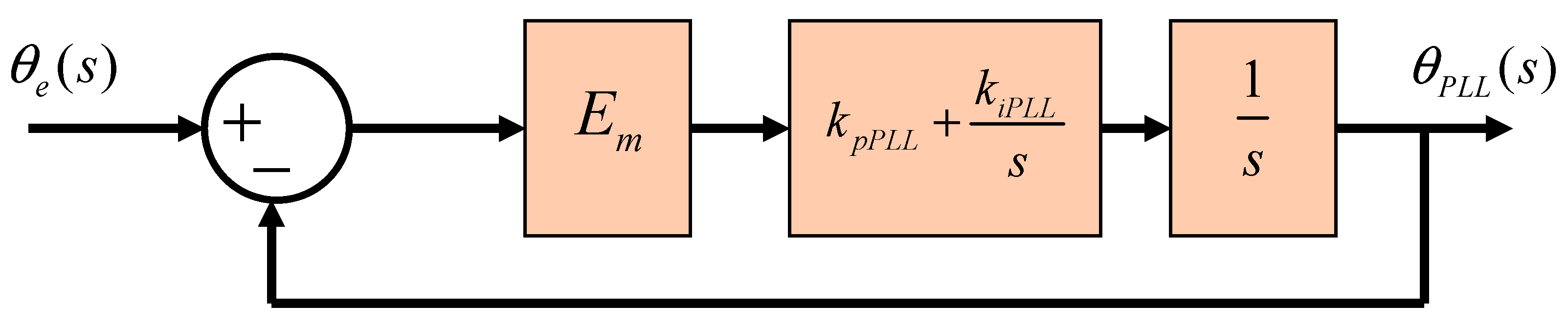
The conventional and simplest PLL design process assumes a simple PLL small signal model and an ideal grid with negligible impedance, i.e.,
. Based on these assumptions, the parameters of the PLL controllers are obtained by Linear Time Invariant (LTI) design methods such as those which use only the desired natural frequency and the damping ratio. However, in weak grids with high
, stability issues initiated by the PLL dynamics may appear, leading to unstable operating modes that will ultimately cause the disconnection of the converter due to the operation of overcurrent or overvoltage protection [
4]. Therefore, the PLL design process should be improved to account for non-negligible grid impedance. In fact, when the grid impedance is high, the PCC voltage depends on the grid voltage, the grid impedance and the current injected by the inverter into the grid. As a result, there is a coupling between the PLL and the grid [
5,
6]. For this reason, above certain grid impedance values, a PLL design neglecting the grid impedance produces unstable behaviour leading to loss of synchronisation. This is a well-known phenomenon that has been addressed by several publications which aim to provide models that explain the interaction between the PLL and a weak grid.
In [
7], a model of a three-phase system in the
dq reference frame considering the effects of the PLL dynamics was proposed. The authors analysed the inverter output impedance and concluded that a high PLL bandwidth increases the negative real part of the impedance and therefore stability issues can appear [
8]. The model presented in [
7] does not consider the coupling terms in the current feedback control. In [
9], the model reported in [
7] was improved by considering the coupling terms, the duty cycle, and the voltage feedback control. It was shown that the PLL bandwidth has an influence on the inverter output impedance
[
9] which behaves as a negative incremental resistor. It should be noted that the model reported in [
9] was evaluated when injecting only active power. The authors in [
10] extended the model proposed in [
9] by considering the injection of reactive power and the effects of a power control loop. Subsequently, in [
11] this model was used together with the generalised Nyquist criterion to study the stability of converters connected to a weak grid with a focus on the PLL parameters. Experimental results validated the proposed stability analysis. In [
12], the authors proposed an improvement in the design of the current controller parameters for an LCL ( An output filter composed by an inductance, a capacitor and an inductance)-type grid-connected converter for reducing the negative effects of the PLL bandwidth on the system stability when the grid is weak. The proposed guideline for the tuning of the current controller was experimentally validated. [
13,
14,
15] used the dynamic phasor to derive an average model of a single-phase inverter feeding into a grid. Based on this model, an output impedance matrix was derived. It was concluded that the imaginary impedance
[
13] is negative for low frequencies because of the presence of the PLL. The Nyquist criterion was then used to predict the stability of the system with different values of PLL integral gain. Only the first order phasors were taken into account - the zero order phasors were not considered leading to a reduction in the model performance. In [
16] a single-phase inverter connected to a weak grid through an LCL filter was studied. Using this system, the output impedance of the inverter was derived taking into account the effects of the PLL and digital control delays. The authors proposed an impedance-phase compensation control scheme by increasing the phase margin of the grid-connected inverter. A similar approach was proposed in [
17], where a novel power-voltage control strategy was proposed based on voltage feedback control of the voltage across the capacitor of the LCL output filter of the inverter. Reference [
17] concluded that the stability of a grid-tied inverter remains unchanged with increasing PLL bandwidth. Finally, in [
18,
19,
20,
21] feedforward control methods were proposed to reduce the impact of the PLL bandwidth on the stability of the system.
These methods all model the output impedance of the converter in the Laplace domain and analyse its dependence on the PLL parameters. The precision of these types of model is appropriate. However, they are not always intuitive, and their complexity is high. Additionally, the Nyquist criterion is the tool normally used to analyse stability issues and therefore a measurement or estimate the output impedance may be required. An alternative approach is to model the whole system in which the converter is connected and derive its state space representation, enabling the use of some of the well-known linear control methods associated with state equations, e.g., eigenvalue analysis, participation matrix, state feedback, etc. In this context, in [
22,
23] a single-phase inverter connected to a weak grid was modelled in the AC frame, and the PLL dynamic response was considered. Since the model was derived in the AC frame, it is linearised using harmonic linearisation techniques leading to a linear time-periodic model. Then, the stability of the system was studied by analysing the eigenvalues of the transition matrix, deriving the stability boundaries. This model requires full knowledge of the system. In [
24], an impedance-conditioning term was proposed for the voltage used by the PLL to improve the stability of the system. To verify this approach, a small signal model of the system in the
dq reference frame was developed. However, the scheme was not experimentalyl validated. A similar scheme was realised in [
25], where a model of the inverter in the
dq reference frame was developed to analyse the performance of the proposed current sharing controller. In [
26], the authors modelled an islanded microgrid composed of two inverters with droop control, considering the PLL design. The accuracy of the proposed model was compared using both simulation and experimental results, finding a good match. Although [
24,
25,
26] have developed small signal models of the system considering the PLL design, the main goal of these works was not to study the effects of the PLL on the stability of the system. As a result, their use is not straightforward, and they usually have a high complexity. In this context, [
27] proposed a small signal model in the
dq reference frame to study the impact of the short-circuit ratio (SCR) and PLL parameters on a VSC-HVDC (A voltage source converter (VSC) used by high-voltage direct current (HVDC) applications) converter. The authors concluded that the PLL parameters, particularly at low SCRs, greatly affect the stability of the converter. However, the work was not validated experimentally. The PLL controller gains were changed to evaluate performance, but a rigorous procedure to obtain appropriate values for these gains was not discussed.
These papers proposed models for studying the stability of the system considering the PLL design. However, their complexity is relatively high, and they perform stability studies using given PLL designs. As yet no-one, to the authors’ knowledge, has reported a systematic procedure to design a PLL for use in a weak grid. In addition, no one has reported a comprehensive study of the effects of the PLL bandwidth on the system stability. Therefore, the contributions of this paper can be summarised as:
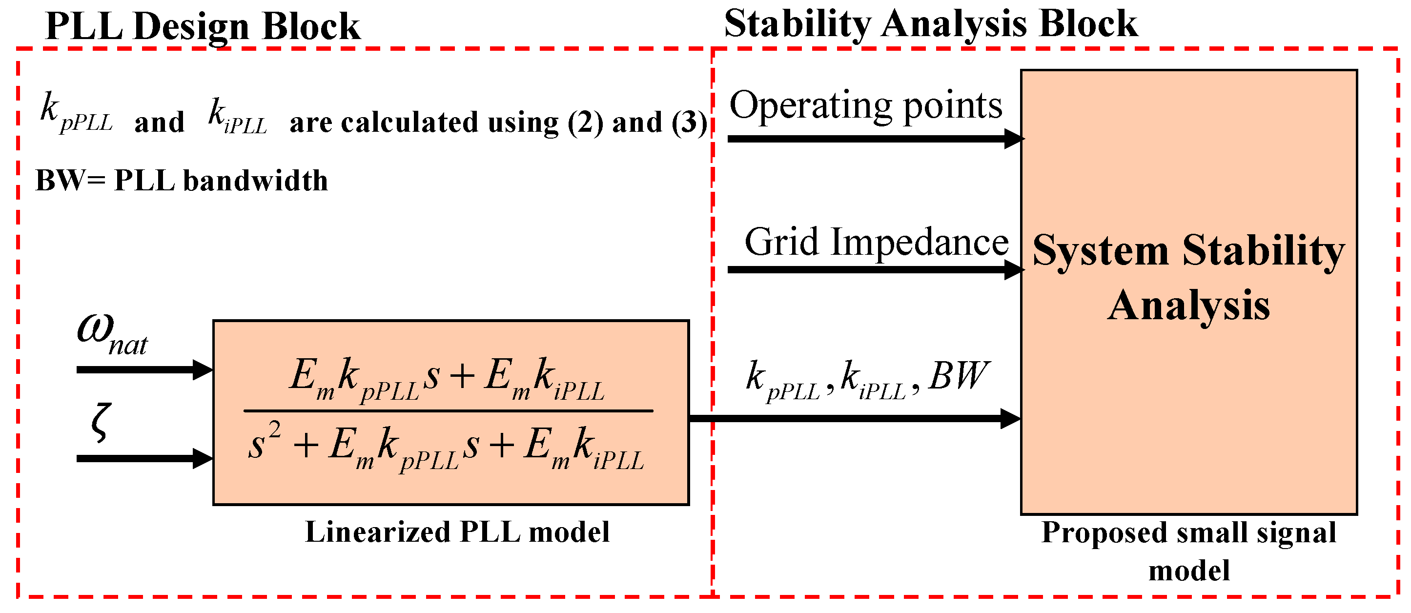
A low-complexity small signal model is proposed for a grid connected converter controlled in the dq reference frame and synchronised with a dq-PLL. This model simplifies the design tasks so that issues such as the PLL bandwidth and the effects produced by a variation of the SCR on the stability of the system can be considered. (the SCR is used to describe the “weakness” of the grid).
Based on the proposed model, a systematic PLL design process is proposed which can be used for balanced, three-phase, three-wire weak grids to ensure system stability.
With the proposed PLL design scheme it is possible to find the maximum bandwidth of the PLL which can be used in the control system for a typical grid-connected power converter, without affecting the system stability.
A comprehensive study of the effects of PLL bandwidth on the system stability is performed. These effects are also studied for different levels of grid weakness. The study presented in this paper has been verified through simulation and validated through extensive experimental work.
The rest of this paper is organised as follows: in
Section 2 the typical
dq-PLL design process is discussed alongside the objectives of the improved design process.
Section 3 introduces the proposed low-complexity small signal model.
Section 4 verifies the stability of the proposed design process using simulation. Finally,
Section 5 reports the experimental validation.
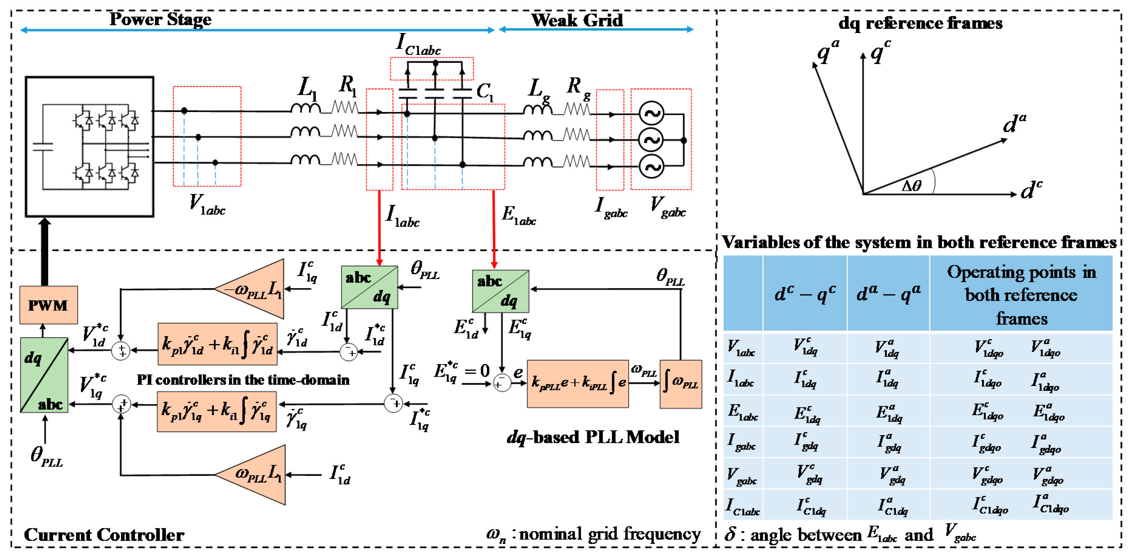
3. Linearised State-Space Model
In this section, the proposed low-complexity small signal model for the non-linear system described in
Figure 3 is developed. To achieve this, two
dq reference frames are defined. The first one is named the converter reference frame (CRF,
) and uses the angle estimated by the PLL (
) from the measured capacitor voltages
in
Figure 3. The second one is the actual reference frame (ARF,
), aligned with the actual angle of the capacitor voltages
. At steady state, the CRF is aligned with the ARF. When small signal perturbations are added to the capacitor voltages (
), CRF and ARF are no longer aligned because of the PLL dynamic response. In this case, the phase relationship between the frames is given by (5). In this equation,
corresponds to the
dq complex variable in the CRF,
is the
dq complex variable in the ARF, and
is the difference between the angle of the ARF and the one of the CRF (see
Figure 3). As shown later in the analysis, this angle allows the easy inclusion of the PLL dynamic response in the system modelling.
It should be highlighted that modelling of the system shown in
Figure 3 is performed considering the fact that the power converter is connected to a balanced three-phase, three-wire weak grid. The proposed PLL design process (
Figure 2) can only be used in this type of system because only the positive sequence is considered in the modelling process. For unbalanced weak grids, both positive and negative sequence components of voltages and currents will circulate in the system, and the proposed model which will be derived in this section should be extended to consider this issue. However, the proposed design scheme shown in
Figure 2 constitutes a starting point to understand the effects of the PLL bandwidth on the stability of the system when the grid is balanced.
3.1. Converter Model in the CRF
3.1.1. Current Control Loop
As shown in
Figure 3, the current control is a conventional
dq control with PI regulators and feed-forward terms. The corresponding state equations are given in (6)–(9) (n the CRF):
Using (6) and (7) in (8) and (9) respectively, the latter two equations can be rewritten as (10) and (11).
Finally, using (6), (7), (10) and (11), the matrix representation of the current control loop of the converter depicted in
Figure 3, in the time domain, is derived. This representation is given by (12) and (13) (in the CRF).
Equations (14), (15) represent the linearised state-space form of (12) and (13) (see [
36,
37]).
and
are the operating points associated to the inverter output current (
), in the “
” reference frame (see
Figure 3);
is the nominal grid frequency and
is a small signal frequency perturbation caused by the PLL algorithm. (More information about the linearisation process is presented in
Appendix A)
3.1.2. LC Filter Model
From
Figure 3, applying Kirchhoff’s Voltage Law (KVL) to the converter side yields (16) (in the
αβ reference frame). In this equation
(voltage at the inverter output),
(current at the inverter output) and
(voltage across the capacitor), where
represents the complex operator:
Transforming (16) to the converter
dq reference frame (see
Appendix B), and rearranging yields (17). Finally, (18) shows the linearised small signal state-space form of (17) [
36,
37] (see
Appendix A):
Assuming that
and
[
26,
36], i.e., the voltage references given by (10) and (11) are effectively produced by the converter, and substituting (15) in (18), yields (19):
3.1.3. PLL and Converter Models
Considering now the PLL and assuming that an instantaneous frequency deviation
exists at the output of the PI controller of the PLL [
7,
25], (20) can be derived in the time-domain. From this equation, a small perturbation in
will produce a small perturbation
at the PLL output. This perturbation will generate a small rotation
between the CRF and the ARF as discussed at the beginning of this section (see
Figure 3). Defining
, (20) can be written in the matrix form shown in (21):
Finally, combining equations (14), (19) and (21), the overall state-space model of the grid-connected converter with current control and PLL, derived in the CRF, is given by (22). It should be pointed out that all the elements in column five of the state matrix are zeros because the state
represents the difference between the converter reference frame and the actual reference frame (see
Figure 3 and (5)). Based on that, and taking into account that until now, all the modelling processes have been performed in the converter reference frame, the state
has no effect on the states shown in (22). Once the actual reference frame is considered in the modelling process, the state
has an effect on more than half of the states of the proposed model, as is shown in (44) where the whole model of the system is presented.
3.2. Converter Model in the ARF
To refer the converter model (22) to the ARF, (5) is used. This equation, as small signal quantities, is given by (23) (see
Appendix A):
In (23), the subscript “
” corresponds to steady state quantities. Note that the angle
is zero in steady-state and therefore, (23) can be rewritten as (24):
are small signal quantities in the CRF.
are small signal quantities in the ARF.
are dependent on the operating point in the ARF. Finally,
is the small perturbation in the angle between the converter and the actual reference frames, that enables the inclusion of the PLL dynamics in the system model (see
Figure 3)
Using (24), voltages (
,
) and currents (
,
) of the converter model shown in (22) can be referred to the ARF as shown in (25) and (26):
In these relationships,
,
and
,
are the currents and voltages at the quiescent operating point in the ARF (currents are measured at the inverter output, see
Figure 3).
Finally, using (25) and (26), and assuming that
, the small signal model in (22) is referred to the ARF to derive the model shown in (27). The assumption
is utilised because the current references are not affected by small variations in the PLL states [
7,
8,
9]:
3.3. System Equations
In this Section, the remaining equations associated with the system in
Figure 3 will be derived. Note that all the equations are in the ARF illustrated in
Figure 3.
3.3.1. Capacitor Equations
From
Figure 3, by applying Kirchhoff’s Current Law (KCL) to the capacitor
, yields (28) (in the αβ reference frame). In this equation,
(voltage across the capacitor),
(current at the inverter output) and
(current grid).
Referring Equation (28) to the actual
dq reference frame (ARF), and rearranging it, yields (29) (see
Appendix B)
Based on (29), the small signal model of the voltage across the capacitor shown in
Figure 3 in the ARF is given by (see
Appendix A):
The output of the inverter model shown in (27) is used in (30) to replace and , leading to (31).
3.3.2. Grid Equations
From
Figure 3, by applying Kirchhoff’s Voltage Law (KVL) to the grid side, yields (32) (in the
αβ reference frame). In this equation
,
and
(grid voltage):
Referring (32) to the actual
dq reference frame, and rearranging it, yields (33) (see
Appendix B)
3.4. Steady State Operating Points
From (27) it is seen that the proposed model requires a steady-state operating point to be evaluated (considering that the system has a non-linear nature). In particular, the operating point of (27) is composed of four variables: these are:
,
,
, and
(see
Figure 3). All of these are defined in the ARF—which is identical to the CRF if steady state operation is considered (assuming that the system is stable). The variable
is equal to zero because the converter control is oriented to the d axis. Moreover, as discussed above, the variables of the operating point associated with the current (
,
), in the ARF, can be approximated with the ones in the CRF:
and
. The remaining variable,
, is derived in this section.
The grid impedance (
) used in this work is mainly inductive and considering that the grid voltage has an angle δ with respect to the capacitor voltage (see
Figure 3), the active power injected to the grid by the converter, can be expressed as shown (35) [
38,
39]. In this equation,
and
, are respectively, the peak values of
and
(see
Figure 3):
Since the control of the converter shown in
Figure 3 is oriented to the d axis (
), it can be shown that
[
40], and therefore the active power given by (35), in the
dq reference frame, can be written as (36):
Finally, using (35) and (36), (37) is obtained. In this equation,
is the grid current in the d axis,
is the nominal frequency of the system, and
is the grid inductance:
Analysing the d axis of (33), in the steady state, yields (38). In this equation,
and
are operating points for the current on the grid side (see
Figure 3). These operating points must be written as a function of the inverter output currents (
,
, see
Figure 3) as shown in (39) and (40) because the converter model of (27) utilises these currents:
Using (40) in (38), yields (41). In this equation,
is the d component of the grid voltage (
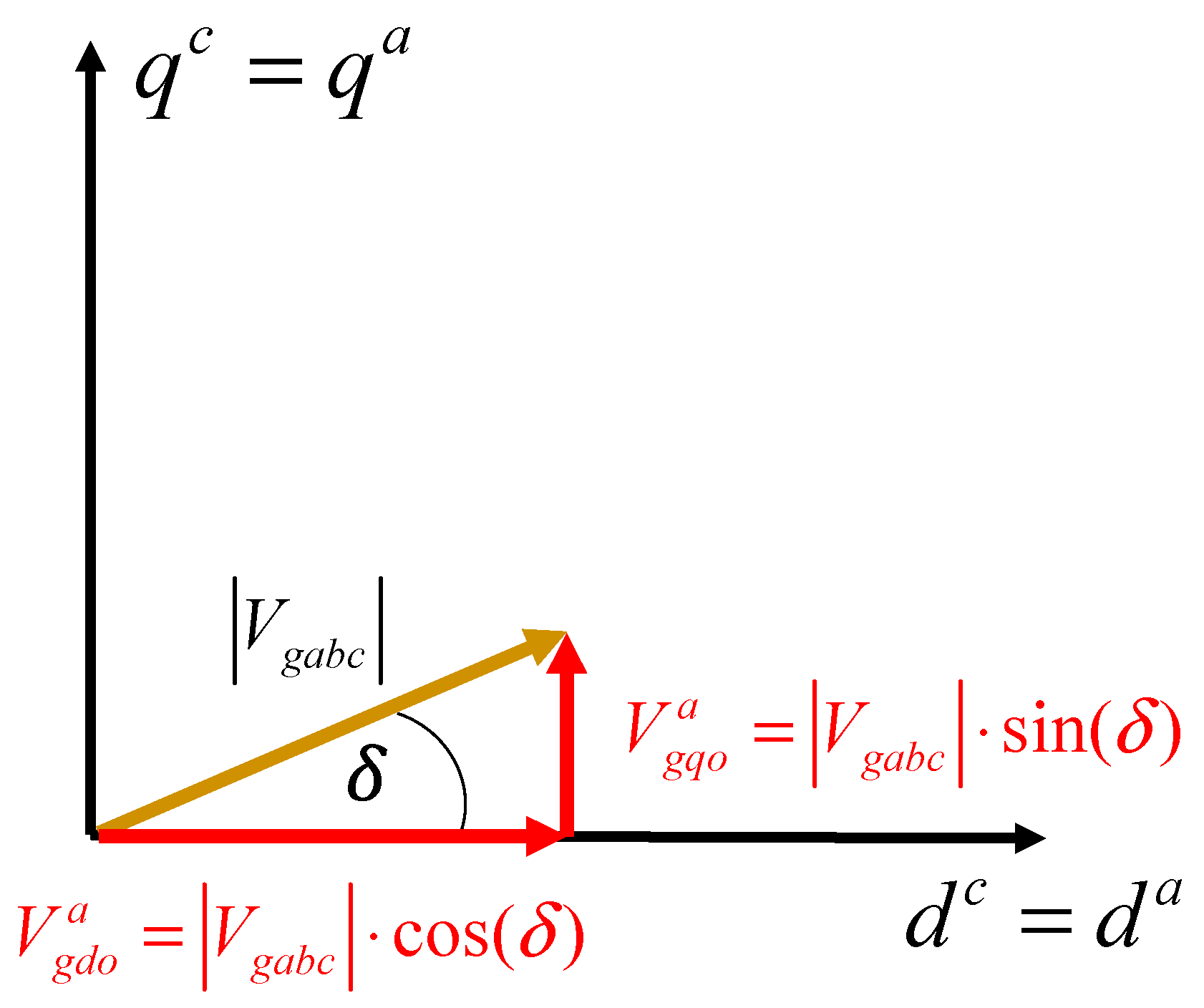
) in the ARF, and it can be calculated using the diagram shown in
Figure 4 as shown (42). In this equation,
is the peak value of the grid voltage, and the angle δ is given by (37) (see
Figure 3). Finally, using (37), (41), and (42) a theoretical expression for
can be obtained (43):
3.5. Whole System Model
Using equations (27), (31) and (34), the whole small signal model of the system shown in
Figure 3 is obtained. This model is shown in (44) and the required operating point (
,
,
,
) is discussed in
Section 3.4. The model can be represented as shown in (45) in the Laplace domain. The stability of the system can be studied by analysing the eigenvalues of the transition matrix “
”. In this work, the stability analysis will be performed as a function of the PLL bandwidth and the weakness of the grid, quantified by the SCR. It is worth noting that if additional outer loops are added for controlling the converter of
Figure 3, (for instance, active or reactive power loops), this will lead to an increase in the number of states of the model depicted in (44) and the system stability can be still studied through the eigenvalues of the extended model. Moreover, it should be pointed out that although the proposed model (44) was used in this work for studying the stability of the system as a function of the PLL bandwidth and the SCR of the grid. This model can also be used to perform other types of stability studies, for example, (i) to improve the design of the current controller of the system (
and
see
Figure 3) when the grid is weak, (ii) to improve the design of the power converter, e.g., providing additional information to calculate the parameters of the second order LC output power filter (An output filter composed by an inductance and a capacitor), taking into account the weakness level of the grid, (iii) for online stability monitoring, among others.
4. Stability Analysis and Simulation Results
Using the small signal model (44), the proposed PLL design methodology for weak grids shown in
Figure 2 can be implemented. In (44), the parameters associated with the inverter output filter and the inverter controllers are kept constant. To study the system stability under different PLL bandwidths, the gains
and
are modified based on the PLL design requirements
and ζ (see the method described in
Section 2.1). Also, the weakness of the grid, characterized by the SCR, is modified using different values for the grid impedance (
, see
Figure 3). Results obtained using (44) are first compared with results from simulating the full system in PLECS (a power electronics simulation package) results to verify the model in an environment where all the parameters are known. The model is later validated experimentally as discussed in
Section 5.
The parameters of the system studied are shown in
Table 1. First, ten PLLs with different bandwidths in the range 10.2 Hz to 102.648 Hz are designed (using the method described in
Section 2.1), obtaining the gains listed in
Table 2. Notice from this table that the phase margin (P.M.) for each design is close to P.M. ≈ 65° to allow a fair comparison. Finally, using the stability analysis block shown in
Figure 2, which is based on the study of the eigenvalues of model (44), the stability of these PLL designs is assessed.
In addition, the small signal model depends on the operating conditions of the inverter, hence stability will change accordingly. For each of the ten PLL designs, it is possible to calculate the maximum active power component of the current that the inverter can inject into the weak grid, before reaching instability, as a function of the PLL bandwidth and the SCR of the grid. The values of
used in this work and the SCRs associated with them are shown in
Table 3.
Unless otherwise stated, it is assumed in this work that the set point for the reactive power component of the current supplied by the converter is zero, i.e.,
(see
Figure 3), i.e., the current supplied by the converter corresponds to the active power component.
Based on this study, it is possible to find the following information about the system stability: (i) the maximum active power component of the current that the inverter can supply to the grid as a function of the PLL bandwidth and the SCR of the grid before going into the unstable zone, (ii) the maximum PLL bandwidth (BW) which can be implemented in the system of
Figure 3 as a function of the grid SCR. Finally, using the proposed PLL design of
Figure 2, it is possible to optimise the PLL design to ensure a fast and stable system operation.
It should be pointed out that the current controller of the inverter shown in
Figure 3 was designed for SCR = 2.5942, and controllers were kept constant for different SCRs. In this case, the closed-loop bandwidth of the current control loop is 200 Hz. The proportional and the integral gains are:
and
(see
Figure 3). These PI controller gains are used to evaluate the model shown in (44). The same controller is used in the simulation work as well as in the experimental work.
4.1. Comparison between Model and Simulation Results
To verify the proposed
dq-PLL design process shown in
Figure 2, in this subsection, a comparison is made of the results achieved with the proposed model and the full system simulation, in terms of stability, as a function of the PLL bandwidth and the grid SCR. The full simulation is implemented in PLECS software, using the non-linear system of
Figure 3 and the parameters listed in
Table 1. However, considering that the proposed small signal model is based on an average model of the inverter, the full simulation model therefore neglects the PWM effects, using controllable voltage sources to represent the converter.
The proposed small signal model is verified studying the eigenvalues of the transition matrix (45). The results are generated as follows: all the PLL designs shown in
Table 2 are evaluated for each of the SCRs shown in
Table 3.
In each condition, the maximum active power current that the inverter can inject into the weak grid before the system becomes unstable is calculated with the proposed analytical model and with the PLECS simulation. Then, theoretical and simulation results are compared. The nominal active current of the inverter shown in
Figure 3 is 18 A. It should be pointed out that to generate
Figure 5 (model results), the linearised model (44) was evaluated for each of the operating points shown in that figure. It is worth remembering that the operating point of (44) is composed of four variables (
,
,
, and
) as discussed in
Section 3.4. In particular,
considering that the control of the converter is orientated along the d axis, i.e.,
. Therefore, only the active power component of the current (
) supplied by the converter into the weak grid is studied. The rest of the operating points for evaluating (44) are generated as follows, Assume that model (44) is evaluated around an active current level of 10 A, which means that
.
is then calculated according (43). Finally, the stability of the system in that operating point can be studied as a function of the PLL bandwidth (by modifying
and
) and the SCR of the weak grid. (By modifying
).
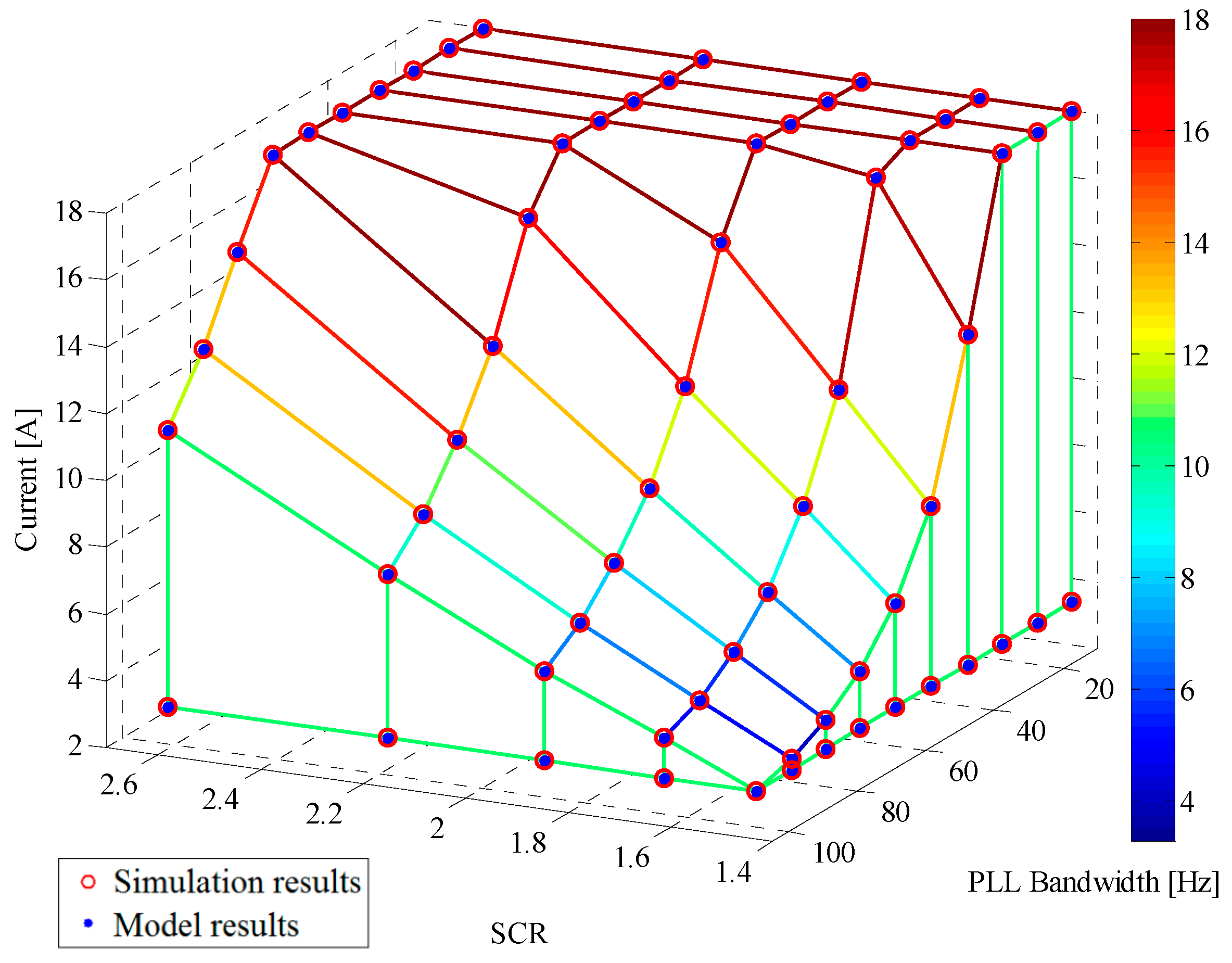
Figure 5 shows the maximum active current—as given by simulations and by the proposed analytical model—that the inverter of
Figure 3 can inject into the grid as a function of the PLL bandwidths described in
Table 2 and for the SCRs shown in
Table 3. Notice that the match between the small signal model and the simulation results obtained from a detailed model implemented in PLECs
® (version 4.1.2, Plexim, Zurich, Swiss) and MATLAB
® (version R2017b, MathWorks, Massachusetts, USA) software, is almost perfect. The figure confirms that the proposed small signal model (44) can effectively represent the effects of the PLL dynamics when the converter operates connected to a weak grid. Moreover, it is possible to conclude that with a high PLL bandwidth and a small SCR, the converter is not able to inject the nominal active current into the grid. In fact, in some conditions, the inverter can supply less than 50% of the rated active current, leading to under-utilisation of the installed power capacity. The proposed design process, shown in
Figure 2, can effectively prevent incorrect PLL designs. For example, if ta renewable energy system is connected to a weak grid with a SCR equal to 1.6265, the proposed model shows that the fastest PLL that can be implemented without affecting the stability and power transfer capability has a bandwidth of about 30 Hz (see
Figure 5).
To use the proposed
dq-PLL design process, it is necessary to have the following information: (i) the parameters of the PI current controllers, (ii) the parameters of the converter output filter and (iii) the weakness of the grid (SCR index). The first two are known because they are characteristics of the converter, while the SCR can be estimated as discussed in [
41,
42].
4.2. Eigenvalue Analysis
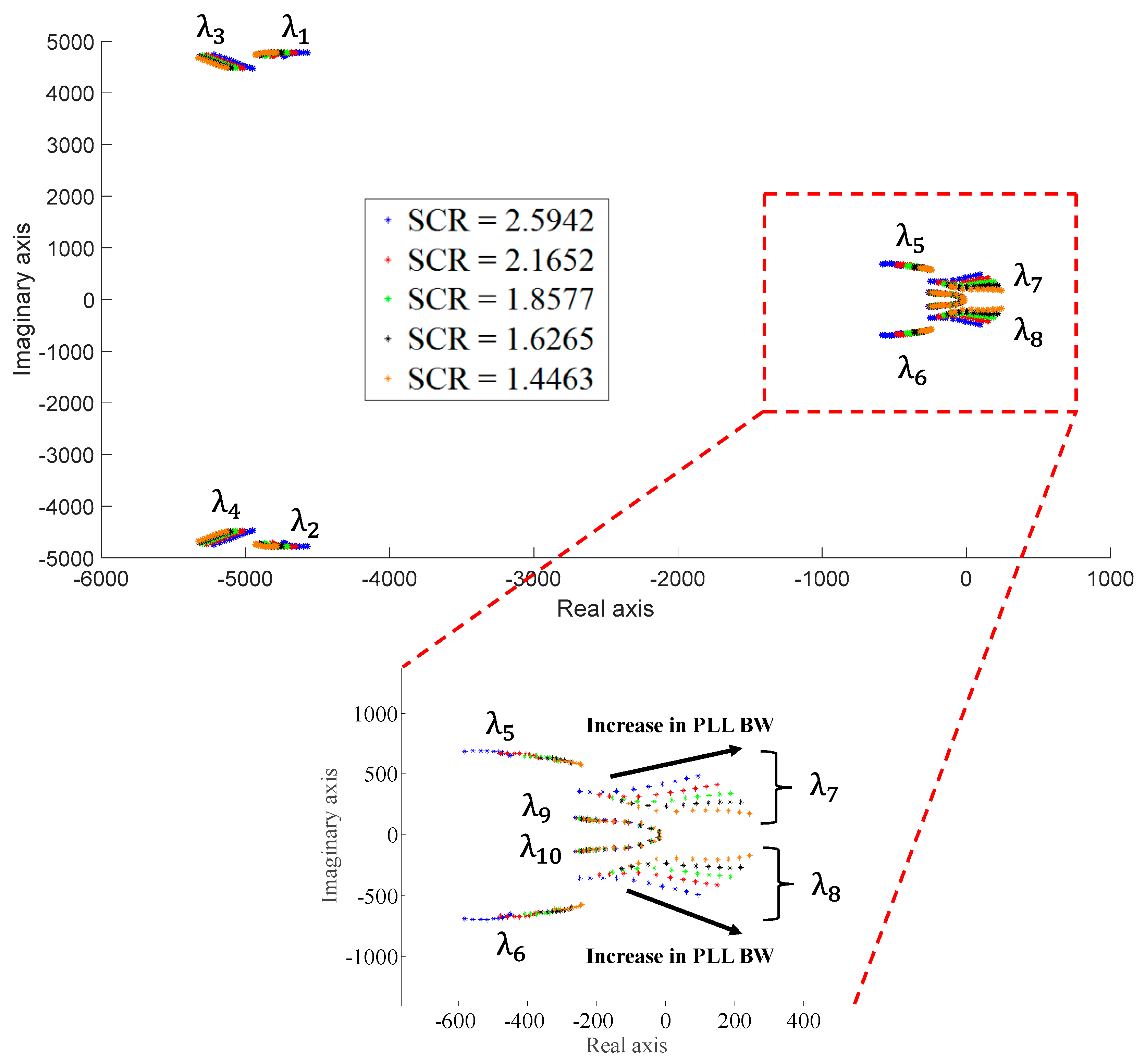
In this section, the eigenvalues of the proposed model (44) are shown as a function of the PLL bandwidth and the grid SCR. The analysis is performed at rated conditions, with the converter injecting the rated active power current (18 A) into the weak grid. The results are shown in
Figure 6, where it is shown that t modes 7 and 8 are heavily affected by the PLL bandwidth and by the SCR of the grid and are responsible for the instability (the rest of the modes do not affect the stability of the system). For this reason, the damping ratio of the proposed model modes as a function of the PLL bandwidth and the SCR of the grid has been calculated. This is performed for the rated conditions of the non-linear system in
Figure 3.
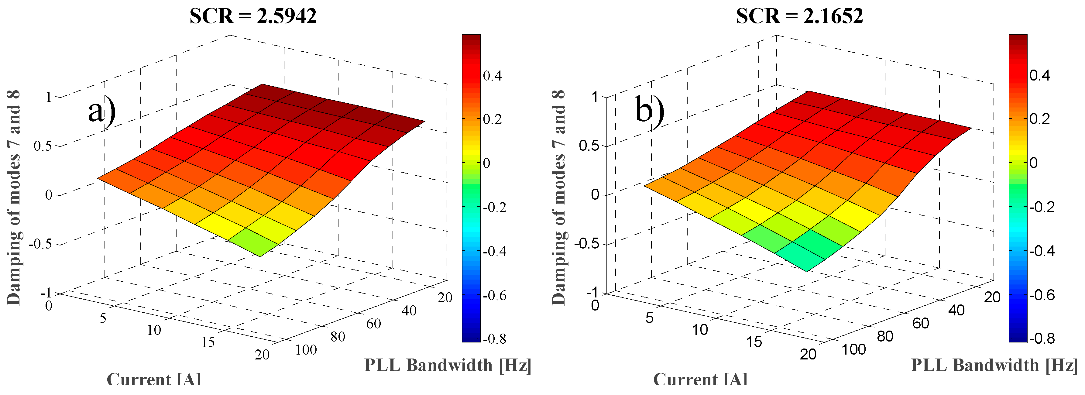
Figure 7 shows the damping ratio of the modes of the proposed model. The damping ratio of modes 7 and 8 are the same for both modes since they are a complex conjugate pair for the ten PLL bandwidths considered (
Table 2) and the different grid SCRs (
Table 3).
Figure 7 shows that for all the SCRs, the damping of modes 7 and 8 is an approximately linear function of the PLL bandwidth, with the damping decreasing as the bandwidth increases. Moreover, the lower the SCR, the sooner the damping crosses the imaginary axis, bringing the system into instability. For the strongest grid, with SCR = 2.5942, the damping crosses the imaginary axis with a PLL bandwidth of 72.136 Hz. For the weakest grid, with SCR = 1.4463, the crossing occurs at 30.898 Hz. (See
Figure 7). Finally, from
Figure 7, it can be concluded that the other modes of the proposed model (those different from modes 7 and 8) do not affect the stability of the system.
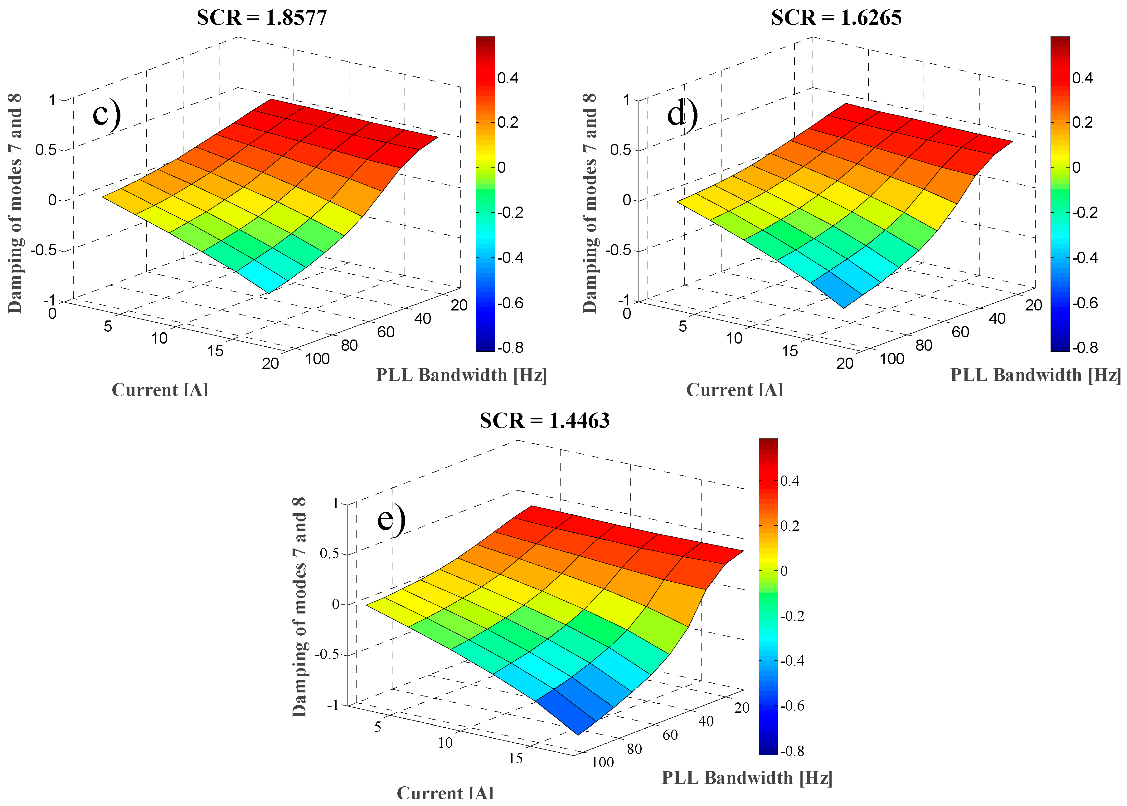
To explore stability for operating points other than rated,
Figure 8 shows the damping ratio of modes 7 and 8 as a function of the PLL bandwidth and the active current supplied by the converter into the grid. It should be noted that to generate
Figure 8, the linearised model (44) was evaluated for each operating point depicted in that figure. The figure shows the results for all the SCRs studied in this work (
Table 3). The figure confirms that stability is adversely affected by the amount of the injected active current, with the damping of the modes decreasing as the current increases. Moreover, the decrease is steeper as the SCR decreases and as the PLL design bandwidth increases.
Finally, the participation factor analysis discussed in [
37] is applied to modes 7 and 8 to understand their relationship with the state variables of the proposed model. Based on this analysis, omitted here for brevity, it is concluded that in the case of a high PLL bandwidth and low SCR, the states
and
which are associated with the PLL model in (44) dominate modes 7 and 8, further confirming that the PLL dynamic is the main cause of instability.
5. Experimental Results
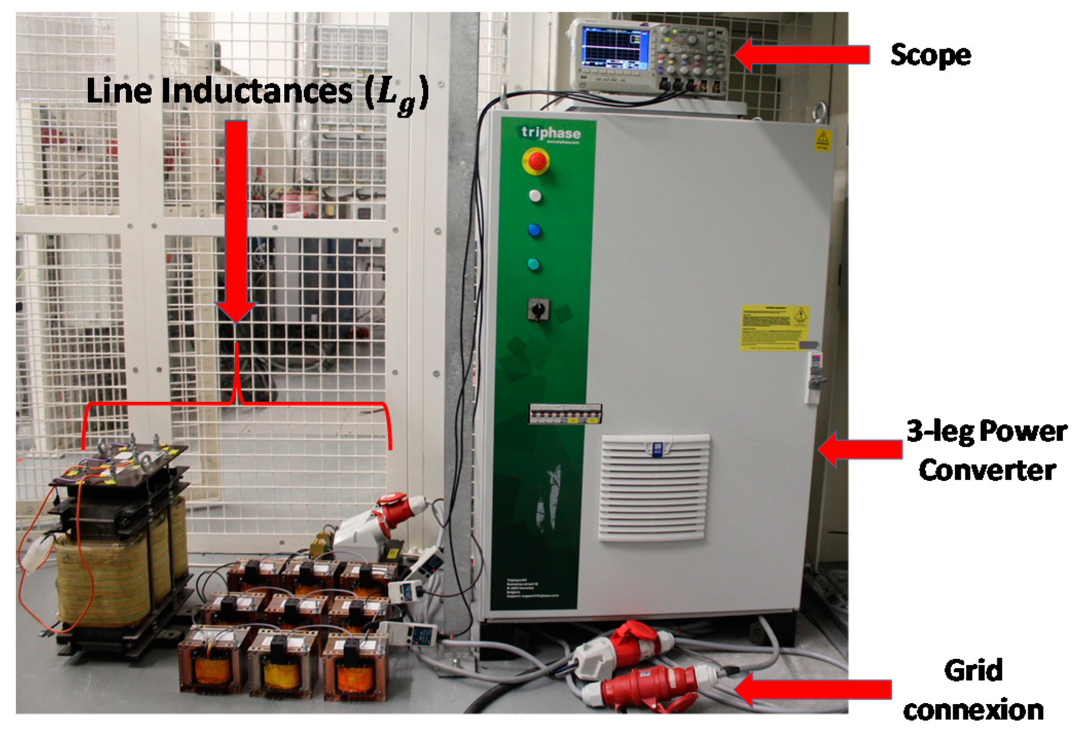
The control system and converter topology of
Figure 3 has been implemented in a Triphase PM15F42C unit (5 kW) [
43,
44,
45] (configured as a 3-leg converter) as is shown in
Figure 9. This unit has the same output filter parameters as those given in
Table 1. Inductances are used to modify the grid impedance, emulating the SCRs described in
Table 3.
The converter is controlled according to the scheme shown in
Figure 3. The same PI gains used in both the simulation and theoretical work described in the previous section are used to control the experimental system. The overcurrent protection of the system shown in
Figure 9 is set at 20 A (instantaneous current).
To validate the proposed small signal model (44), PLL bandwidths in the range of approximately [10–50 Hz] (
Table 2) are considered. These values are used because it is the typical bandwidth of PLLs implemented in a real-life application [
28,
29,
46]. Moreover, all the SCRs shown in
Table 3 are emulated in the experimental rig. First, the maximum active current that the converter can inject into the grid as a function of the PLL bandwidth and the SCR is experimentally measured and compared with that predicted by the proposed model. In the experimental tests shown in this section, current steps of 1A around the quiescent operating points are used. According to the model results described in
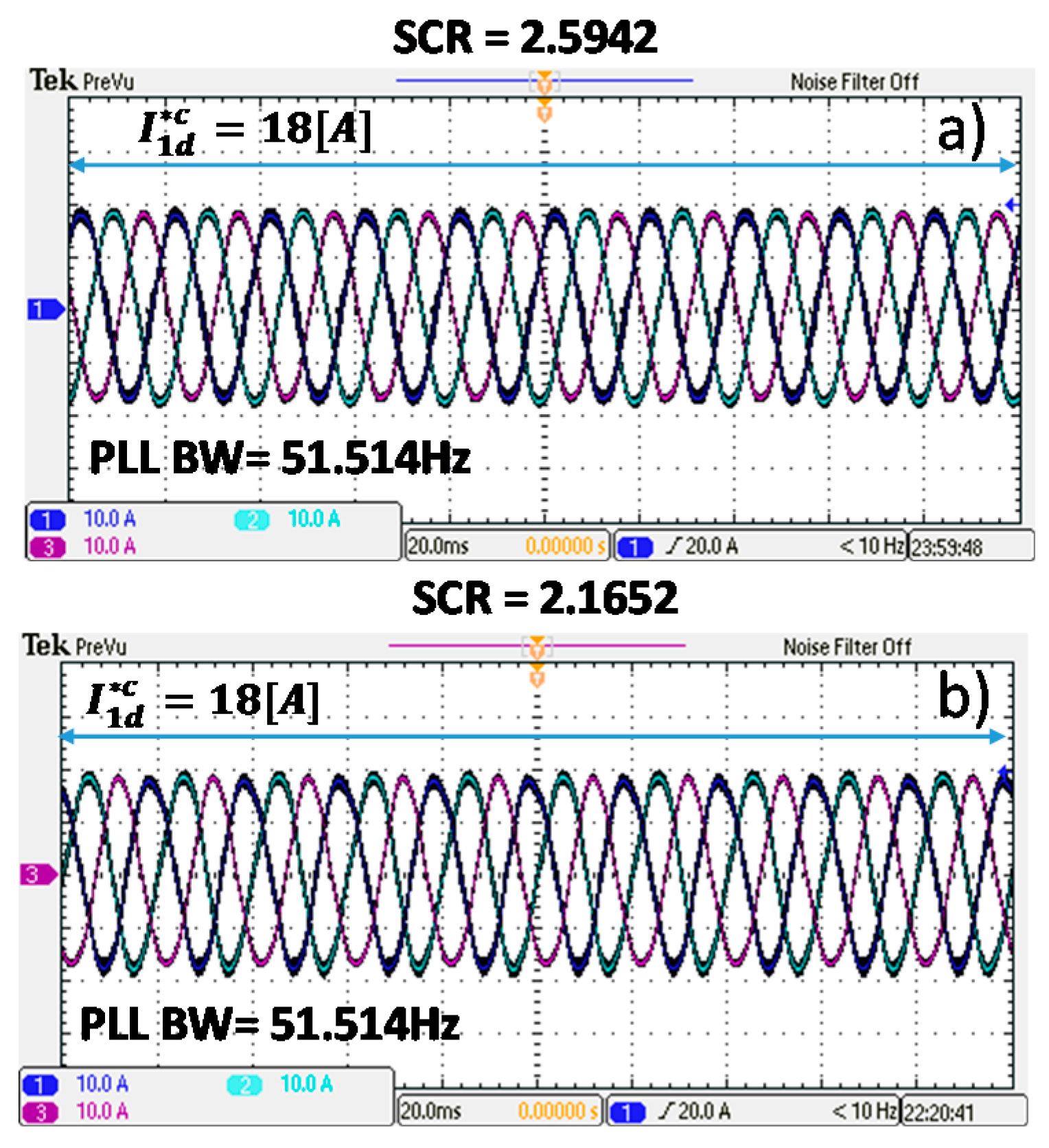
Section 4, the experimental converter can supply the nominal active current (18 A) into the grid without becoming unstable when SCRs of 2.5942 and 2.1652 are used. This occurs for the whole range of PLL bandwidths, [≈10–50 Hz].
Figure 10a shows the nominal active current injected by the inverter for the worst case, i.e., for a PLL bandwidth of ≈51.5 Hz. The same trend is shown in
Figure 10b where the SCR of the grid is equal to 2.1652. In this case, the parameters of the PLL implemented in the converter of
Figure 9 are the same parameters used to generate the experimental results shown in
Figure 10a.
In
Table 4, the predictions from the proposed model are compared with the experimental results for a grid with an SCR = 1.8577. When a PLL with bandwidth 51.514 Hz is used, the proposed theoretical model predicts a maximum active current at the converter output of 15.7 A. The maximum active current that the experimental system can inject to the grid without becoming unstable is 14.5 A.
Figure 11b shows that the system is stable when injecting 14.5 A.
When the reference current is changed to 15.5 A (current step of 1 A), the system becomes unstable, showing a good match with the theoretical prediction. If the PLL bandwidth is reduced below 40.723 Hz, the instability issue is avoided, and the converter can fully supply the nominal current to the grid, as shown in
Figure 11a.
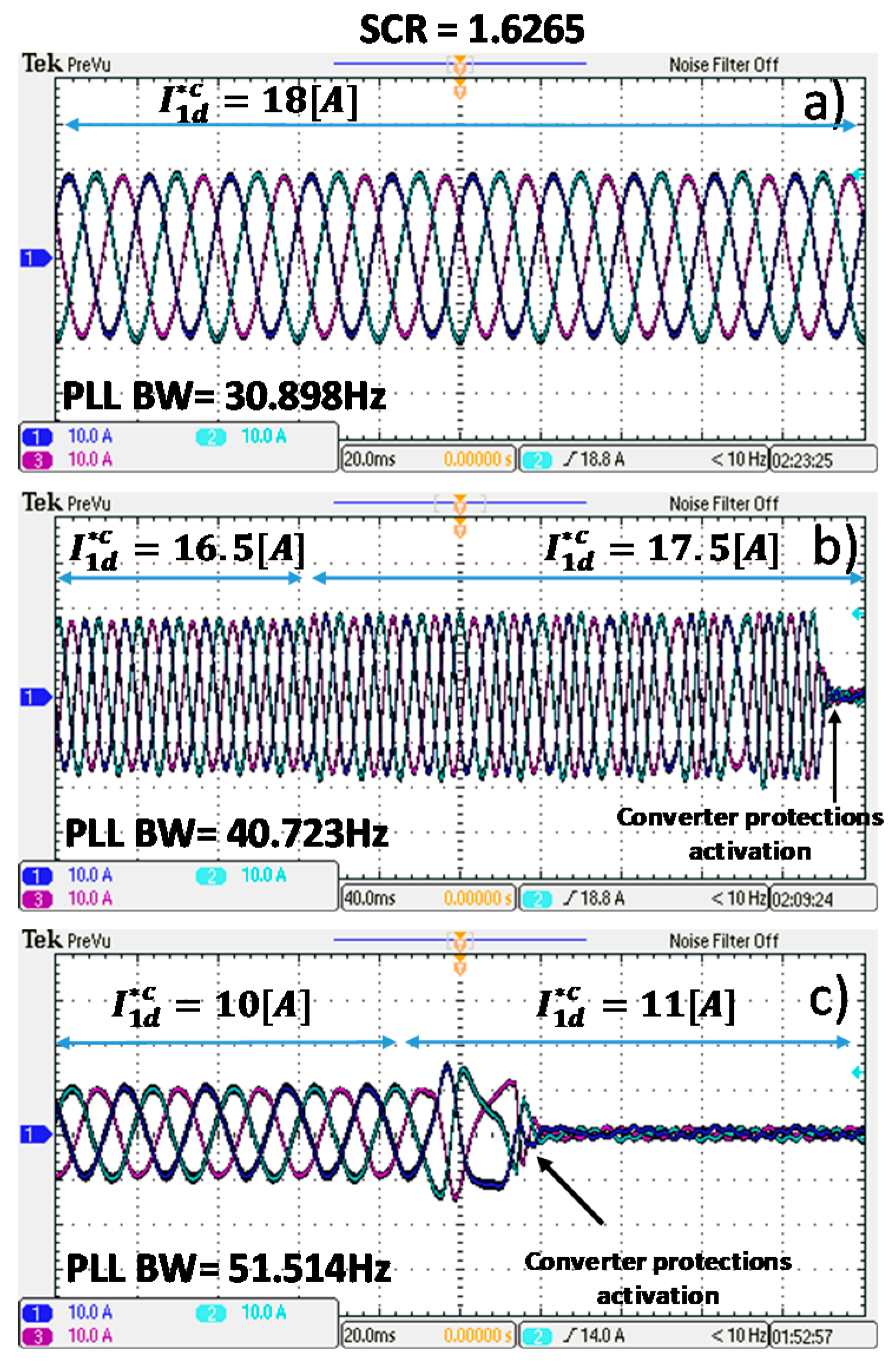
In
Table 5, the experimental results are compared with those produced by the theoretical model for the case of SCR = 1.6265, confirming the good match between the model and the experimental work.
Figure 12 shows the experimental current waveforms corresponding to the three limit conditions shown in
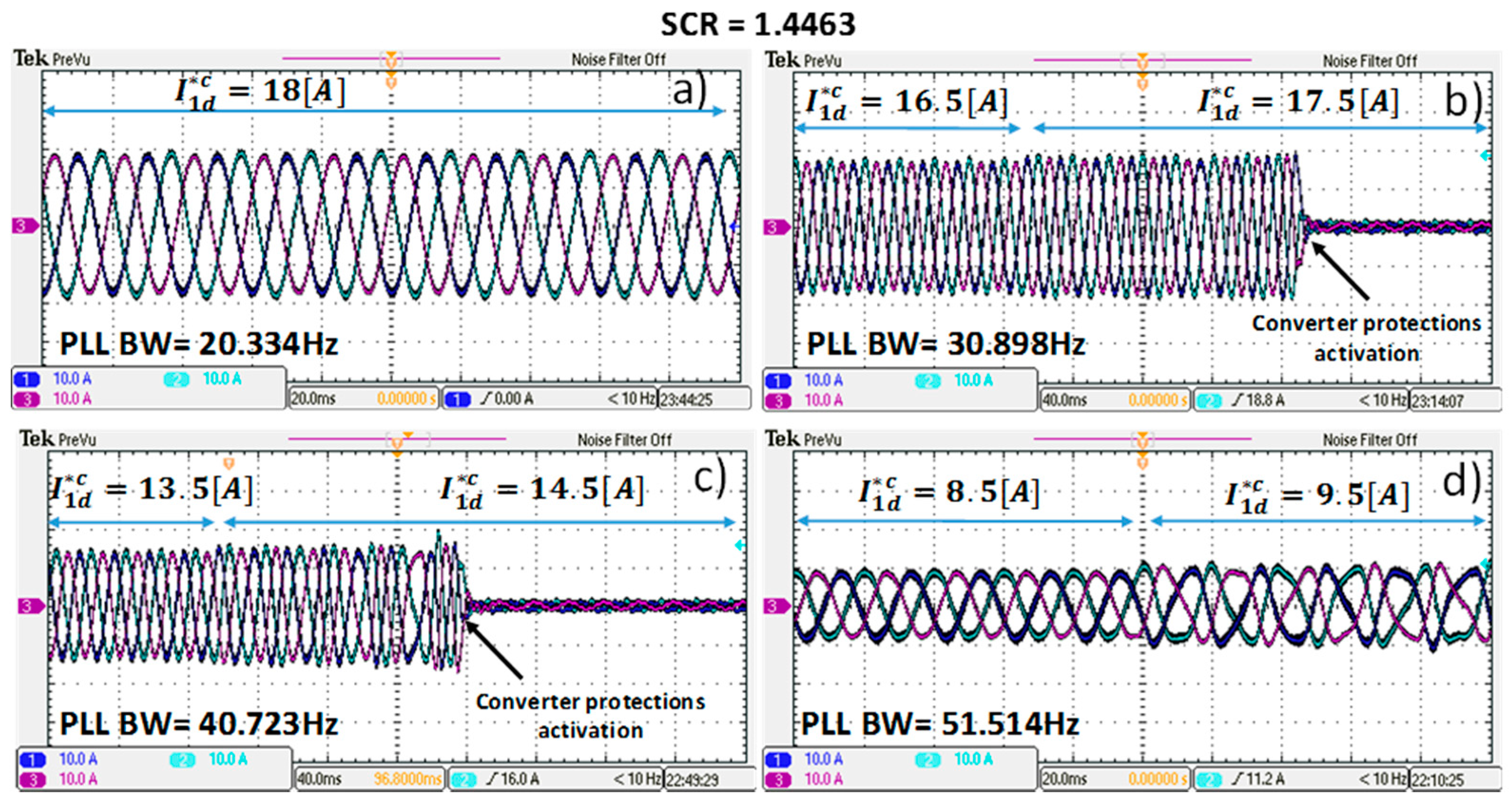
Table 5. For the rest of the cases, the converter can inject its nominal active current. The last case studied uses a SCR of 1.4463, representing a very weak grid. Both model results and experimental results are shown in
Table 6, again confirming that experimental results agree with the theoretical expectations. For instance, if a PLL with a bandwidth of 51.514 Hz is used in the experimental system, the active current that the inverter can inject into the weak grid before becoming unstable is less than the 50% of its nominal current. This case is shown in
Figure 13d where the currents of the experimental rig are presented. To ensure the system stability in nominal conditions, a PLL with a maximum bandwidth of 20.334 Hz must be used as shown in
Figure 13a. Finally, the current waveforms supplied by the converter when the PLL has a bandwidth of 30.898 Hz, and 40.723 Hz are shown in
Figure 13b,c respectively.
In
Figure 14 the frequencies estimated by the PLL (i.e., PLL output) for the cases described in
Figure 12b and
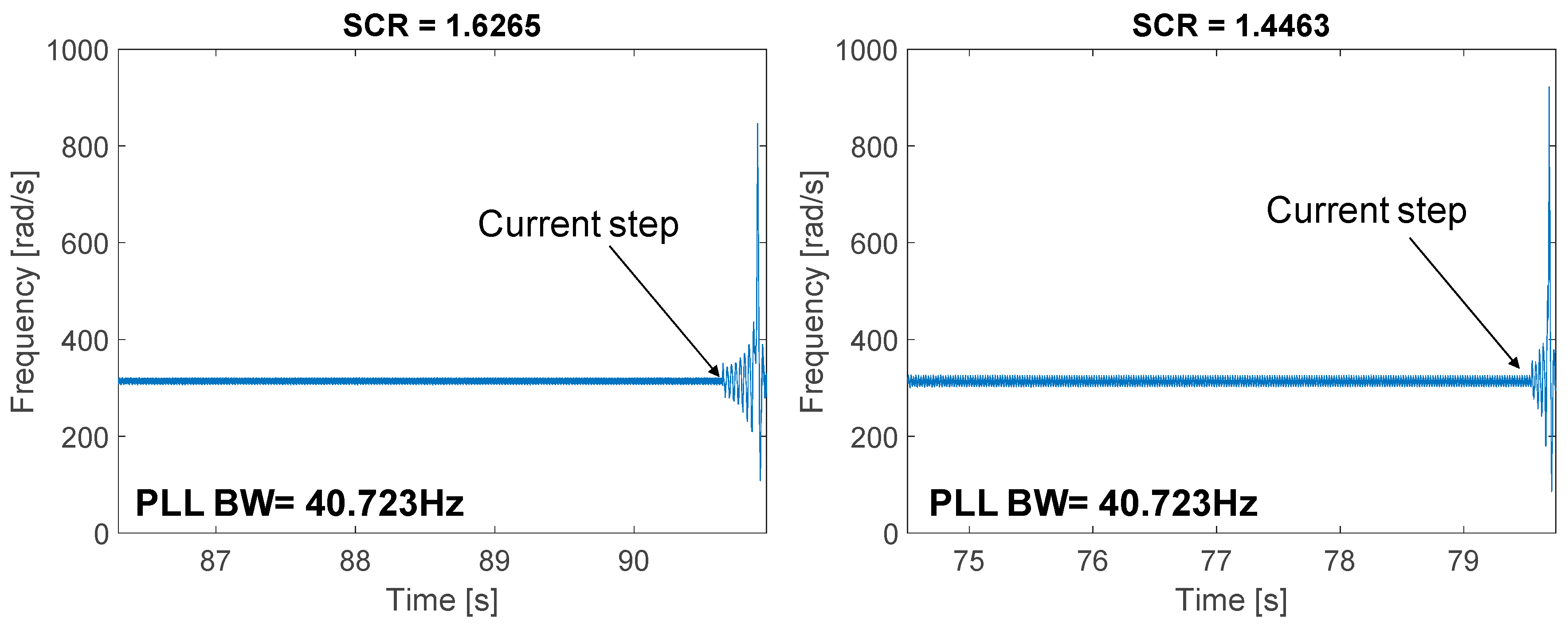
Figure 13c are shown. From this figure, it is concluded that when a step is applied to the active current, for both cases, the frequency at the PLL increases rapidly, driving the system to instability and finally producing the disconnection of the converter from the grid after the operation of the overcurrent protection. It is, therefore, possible to conclude that the proposed model (44) can effectively predict the system stability when the PLL bandwidth and the SCR of the weak grid are taken into account.
The experimental tests presented validate some of the operating points shown in
Figure 5. For completeness, in this section, the experimental validation of the pattern discussed in
Section 4.2 and depicted in
Figure 8 is provided. In
Section 4.2 it was concluded that the stability of the system is adversely affected by increasing the active current injected by the converter to the weak grid, decreasing the SCR, and increasing of the PLL bandwidth. Indeed, from
Figure 8, it can be seen that for a given SCR and PLL BW, the damping of modes 7 and 8 decreases as the active current increases. Based on that, and considering that the settling time of the system is strongly affected by the damping of the dominant modes (those which affect the stability, in this case, modes 7 and 8 of the proposed model), additional experimental tests are now discussed.
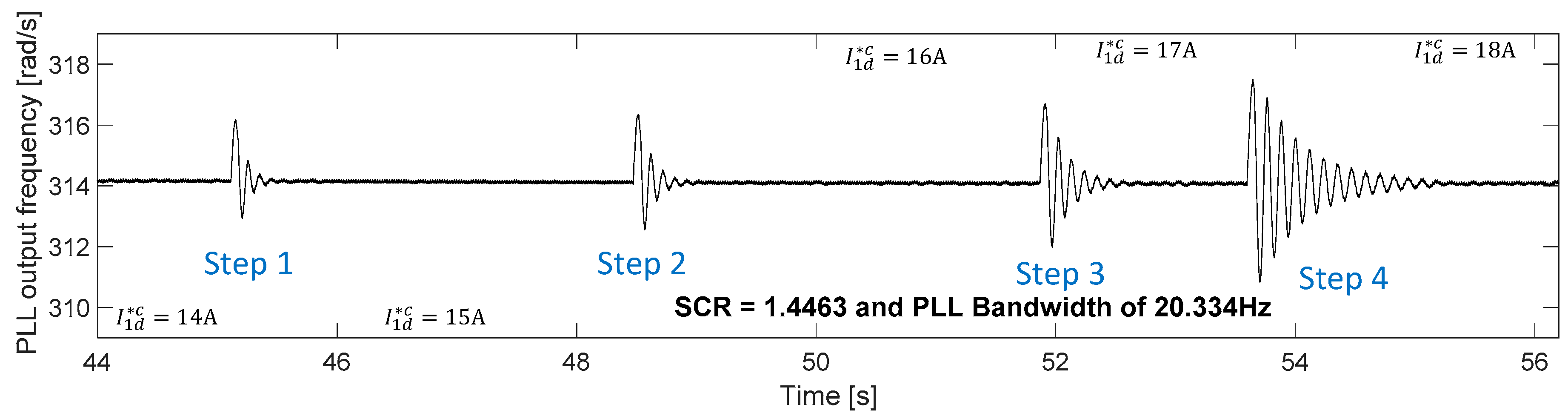
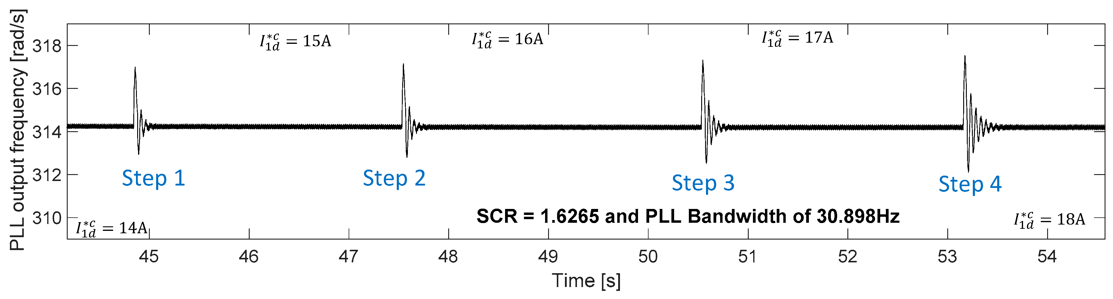
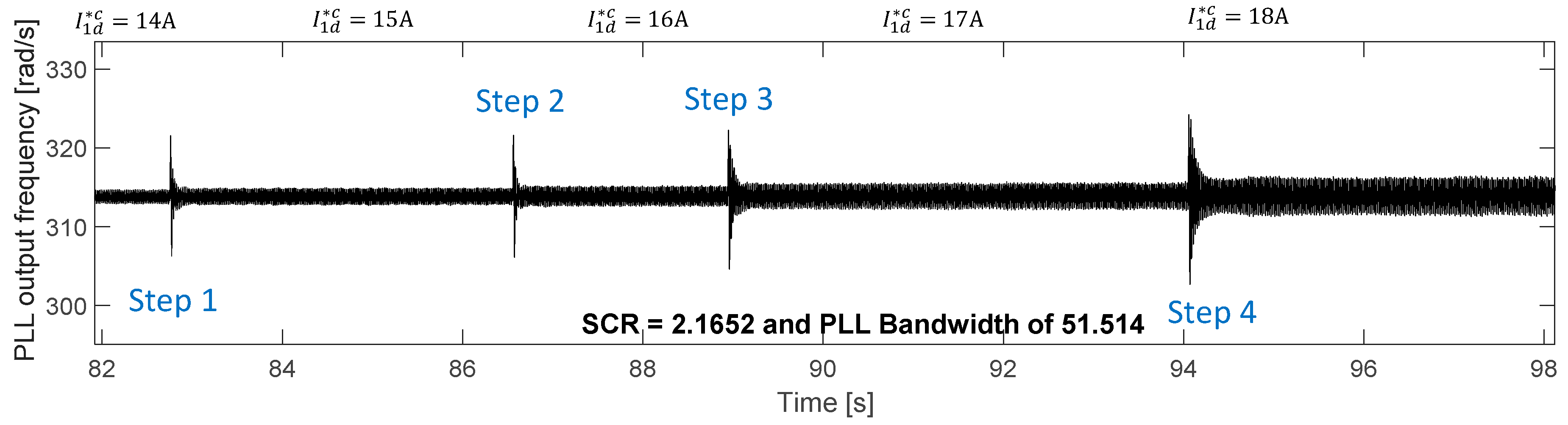
In these tests, the transient response (settling time) of the frequency at the PLL output is studied as a function of (i) the PLL bandwidth, (ii) the SCR of the weak grid, (ii) and for different values of active current. The SCRs considered are 1.4463, 1.6265, 1.8577 and 2.1652. The PLL bandwidths studied are 20.334 Hz, 30.898 Hz, 40.723 Hz and 51.514 Hz. Finally, the following active currents were considered: 14 A, 15 A, 16 A, 17 A and 18 A. The experimental tests were generated as follows: with the experimental system of
Figure 9 working for a given SCR of the grid and for a given PLL bandwidth, the evolution of the frequency at the PLL output is measured and saved online by the Triphase data logging system, for the following current steps:
- ✓
Step 1: The reference value in the converter is changed from to
- ✓
Step 2: The reference value in the converter is changed from to
- ✓
Step 3: The reference value in the converter is changed from to
- ✓
Step 4: The reference value in the converter is changed from to
In all of these current steps, the settling time of the frequency at the PLL output and the frequency of the oscillations in the transient state of this signal are shown. Based on this information, and considering that in those steps, the transient behaviour is dominated by modes 7 and 8 as shown in
Figure 6 and
Figure 8, it is possible to estimate the experimental damping ratio of modes 7 and 8 performing a comparison with those obtained using the proposed model, for the same operating point. In
Appendix C, the procedure to estimate the damping of the modes from the step-response of the system is presented. Using this procedure, the experimental damping of modes 7 and 8 are estimated for the four steps studied and for the operating conditions shown in
Figure 15,
Figure 16,
Figure 17 and
Figure 18. Finally, these experimentally measured damping factors are compared with those calculated using the proposed model (44) as shown in
Table 7,
Table 8,
Table 9 and
Table 10.
It can be seen that the theoretical and experimental damping values of modes 7 and 8 given in
Table 7,
Table 8,
Table 9 and
Table 10 are very close. The differences can be explained for the following reasons: (i) some phenomena present in the actual system were not considered in the modelling process (losses, switching, etc.), (ii) the procedure to estimate the damping coefficient experimentally assumes (see
Appendix C) that only the dominant poles affect the transient state, however others poles may have an effect on the dynamic response of the system. Moreover, when the system is close to instability, small changes in the operating current may produce relatively large changes in the damping coefficient, and this makes the experimental estimation difficult. However, the damping coefficients obtained from the model and the experimental work are very similar, with an error |
ζmodel −
ζexperimental| < 0.1 in all the operating range. The error is much lower when the system is operating with damping coefficients above a given threshold (e.g., 0.25).
Finally,
Figure 15 shows the variation and oscillations at the output of the PLL, in the experimental rig of
Figure 9, for the 4 steps studied. From this figure, it can be concluded that the settling time increases with an increase of the active current
injected by the converter into the weak grid. The same behaviour is seen when analysing the experimental tests shown in
Figure 16,
Figure 17, and
Figure 18. Based on the results given in
Table 7,
Table 8,
Table 9 and
Table 10, this behaviour is because the damping of modes 7 and 8 decreases with an increase of the active current
, bringing the system closer to the zone of instability, and therefore increasing the settling time. Notice that the 2% settling time is usually estimated as
ts ≈ 4/(
ζωn) where
is the damping coefficient and
is the natural frequency of the dominant poles.
6. Conclusions
A low-complexity small signal model of the system has been proposed which includes the PLL bandwidth and the weakness of the grid. The proposed model has been extensively verified with simulations implemented in PLECS and validated experimentally for a wide range of PLL bandwidths and different SCRs.
A dq-PLL design procedure based on the proposed model has been proposed to ensure the stability of converters connected to weak grids. The improvement of the proposed design scheme over the schemes reported in previous studies is the fact that (to the best of our knowledge), this is the first paper where a systematic procedure to design a PLL to be used in weak grids is proposed.
Experimental results obtained from a 5 kW laboratory scale system confirm that the proposed model and design process can be effective tools to optimise the system operation in terms of finding the fastest PLL that can be used in a weak grid with known SCR without affecting the system stability. The small differences between both model and experimental results can be justified because phenomena present in the experimental rig (e.g., losses, switching) were not taking into account in the proposed model or in the assumptions used in the modelling process. (See
Section 3)
The fact that the proposed model is simple enables it to be used for online stability monitoring. In fact, only modes 7 and 8 of the model are affected by the PLL bandwidth and the SCR of the grid. If an algorithm for monitoring the grid impedance is added, the stability of the system can be monitored online through the calculation of modes 7 and 8.
The proposed PLL design process is suitable for three-phase three-wire balanced weak grids. Its extension to consider unbalanced and/or harmonic weak grids is proposed for future work. In unbalanced weak grids, it is necessary to consider both positive and negative sequence components of currents and voltages of the system in the modelling process. In harmonic weak grids, it is necessary to consider the voltages and currents of the main harmonics present in the system in the modelling process.

 ,
, 


