A Nonlinear Analytical Algorithm for Predicting the Probabilistic Mass Flow of a Radial District Heating Network

Abstract

This paper develops a nonlinear analytical algorithm for predicting the probabilistic mass flow of radial district heating networks based on the principle of heat transfer and basic pipe network theory. The use of a nonlinear mass flow model provides more accurate probabilistic operation information for district heating networks with stochastic heat demands than existing probabilistic power flow analytical algorithms based on a linear mass flow model. Moreover, the computation is efficient because our approach does not require repeated nonlinear mass flow calculations. Test results on a 23-node district heating network case indicate that the proposed approach provides an accurate and efficient estimation of probabilistic operation conditions.

1. Introduction

The development of a low-carbon sustainable energy system has generated increasing interest since energy and environmental issues have become more prominent globally. The present direction of this development has focused on integrated energy systems (IESs) that integrate various energy-related tasks, such as cooling and heating, and various forms of energy, such as electricity and natural gas, to provide a comprehensive utilization and management of energy [1]. However, the increasing integration of energy systems, such as combined heat and power (CHP), gas turbines, and other energy conversion facilities, has greatly increased their interdependence [2,3]. This interdependence necessitates increasingly sophisticated planning and operation of energy systems.

Presently, the planning and operation of IESs is generally based on the steady-state modeling and analysis of IESs. For example, Liu et al. [4,5] established a steady-state model between electricity and heating networks and proposed an effective mass flow calculation method. Similarly, steady-state energy-flow analysis between electricity and natural gas networks has been conducted [6,7]. Moreover, steady-state energy flow analysis has been conducted with integrated electricity-gas-heat systems [8,9,10]. However, steady-state analyses are essentially deterministic and cannot effectively address the many uncertainties arising in IESs, such as random fluctuations in cooling, heating, electricity, and natural gas loads; intermittent energy output fluctuations; generator failures; electric transmission line and gas pipeline failures; and market uncertainties. Moreover, different energy networks have different mutual influences affecting their interdependencies. These studies highlight the necessity of investigating the planning and operation problem of gas/heat systems that are interdependent with power systems.

Recently, numerous studies have sought to develop analysis methods capable of addressing the influence of uncertainties on power networks [11,12,13]. For example, Chen et al. [14] considered the uncertainties of electricity, gas, and heat loads and wind farm outputs within the framework of steady-state energy flows and employed Monte Carlo simulations to solve the probabilistic energy flow of IESs. The effects of various uncertainties on IES reliability have also been studied [15]. A probabilistic steady-state analysis of integrated electricity, gas, and heating networks has been proposed based on Latin hypercube sampling and the Nataf transformation [16]. A stochastic scheduling model is proposed for the interconnected EHs considering integrated demand response (DR) and wind variation [17]. In addition, ensemble prediction systems (EPSs) have laid a foundation for the quantitative analysis and evaluation of the influence of uncertain factors in IESs. In an EPS, the statistical characteristics of random output variables can be obtained according to the statistical characteristics of random input variables by the calculation of probabilistic flows. The methods for solving probabilistic flows include simulation methods [18,19], analytical methods [20,21], and approximation methods [22,23,24]. Monte Carlo simulation is the most common simulation method employed to test the accuracy of probabilistic power flows. The middle semi-invariant method is the most widely employed analytical method owing to its high calculation efficiency. Finally, the most representative point estimation method represents a very commonly adopted approximation method because it requires no knowledge regarding the specific functional relationship between input quantity and output quantity. At present, the probabilistic power flow calculation in power systems has been extensively investigated. However, it should be clarified that few studies have investigated probabilistic mass flows in thermal systems. Moreover, usage of nonlinear analytical algorithms for solving probabilistic mass flows has not been discussed.

The present work addresses these deficiencies in past works by developing a nonlinear analytical algorithm for predicting the probabilistic mass flow of a radial district heating network based on the principle of heat transfer and basic pipe network theory. First, the variance of mass flow through a pipe connected with a heat source is obtained according to the power balance equation of a district heating network. Then, the functional relationship between the mass flow variances between pipes in the network is deduced to obtain the variance of mass flow in the entire pipe network. Second, a functional expression of the pipe network node temperature is derived, and the covariance matrix of the mass flow through the pipe network is obtained. Finally, the variance of the node temperature can be obtained. The validity and rationality of the proposed algorithm is verified by application to a 23-node radial district heating network with various pipe lengths under thermal load fluctuations of various magnitudes. The probabilistic results obtained can provide comprehensive information of real-time IES operating conditions, which is valuable for IES planning, operations, and risk assessment.

2. Probabilistic Energy Flow Model of a Radial District Heating Network

2.1. Steady-State District Heating Network Model

The steady-state model of a district heating network includes a hydraulic model and a thermodynamic model. The hydraulic model includes the joint flow equilibrium equation and the pressure head loss equation, which are, respectively, expressed as follows:

$$\mathit{A}\mathit{m}={\mathit{m}}_{\mathrm{q}}$$

(1)

$${\mathit{h}}_{\mathrm{f}}=\mathit{K}\mathit{m}\left|\mathit{m}\right|.$$

(2)

where, A is the node-branch incidence matrix. m and m_q represents, respectively, vectors of mass flow rate within each pipe and the injected mass flow at the nodes (kg/s). h_f represents the vector of head losses (m), and K represents the vector of resistance coefficient of pipes. The thermodynamic model includes the thermal load power equation, the pipe temperature change equation, and the node power conservation equation, which are, respectively, given as follows:

$$\mathit{\Phi }={\mathrm{C}}_{\mathrm{p}}{\mathit{m}}_{\mathrm{q}}({\mathit{T}}_{\mathrm{s}}-{\mathit{T}}_{\mathrm{o}})$$

(3)

$${\mathit{T}}_{\mathrm{end}}=({\mathit{T}}_{\mathrm{start}}-{\mathit{T}}_a)e^{-hL/({\mathrm{C}}_{\mathrm{p}}m)}+{\mathit{T}}_a$$

(4)

$$({\displaystyle \sum {\mathit{m}}_{\mathrm{out}}}){\mathit{T}}_{\mathrm{out}}={\displaystyle \sum ({\mathit{m}}_{\mathrm{in}}{\mathit{T}}_{\mathrm{in}})}.$$

(5)

where Φ represents the vector of the heat power consumed or supplied (MW). C_p is the specific heat of water, and C_p = 4182 × 10⁻³ MJ·kg⁻¹·°C⁻¹. T_s represents the vector of supply temperatures at nodes (°C). T_o represents the vector of the outlet temperature of flow at the outlet of nodes before mixing in the return network (°C). T_start and T_end represents the temperatures at the start node and end node of the pipe, respectively (°C). h represents the total heat transfer coefficient per unit length (W/(m·k)). L represents the length of the pipe (m). T_a represents the ambient temperature (°C). m_out and m_in are, respectively, the mass flow rate leaving and entering the node (kg/s). T_out represents the mixture temperature at the node (°C), and T_in represents the temperature of mass flow entering the mixing node at the end of the incoming pipe (°C).

Equations (1)–(5) are nonlinear equations, where the coupling relationship between temperature and mass flow is strong, and exponential terms are involved. Therefore, solving these equations for realistic thermal pipe networks directly is quite difficult owing to the high computational complexity involved and the inability for ensuring numerical stability.

2.2. Probabilistic Thermal Load Model

In general, thermal loads can be described probabilistically in terms of a normal distribution. Accordingly, the thermal load probability density function (PDF) can be described as:

$$f(\phi )=\frac{1}{\sqrt{2\mathsf{\pi }}{\sigma }_{\mathsf{\phi }}}\exp [-\frac{{(\phi -{\mu }_{\mathsf{\phi }})}^2}{2{\sigma }_{\mathsf{\phi }}^2}],$$

(6)

where μ_φ and σ_φ are the respective mean and standard deviation of thermal load φ.

2.3. Approximate Model of Probabilistic Mass Flow in a Radial District Heating Network

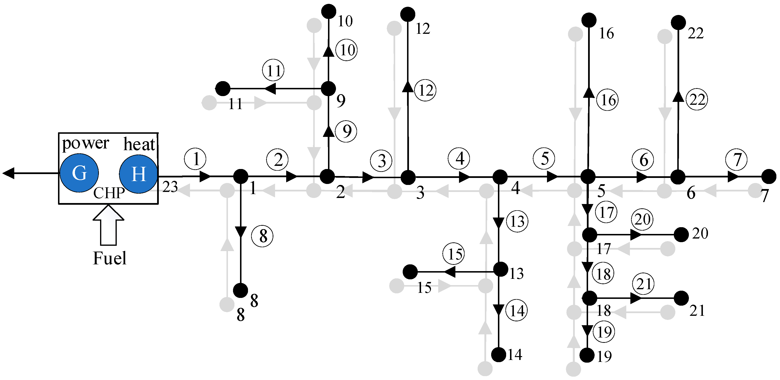
An approximate model of probabilistic mass flow in a radial district heating network consisting of a heat source node H, three pipes, and three nodes is shown in Figure 1. Here, the circled values represent pipes, and the arrows represent the direction of mass flow rates. As demonstrated in Appendix A, the heat loss of a pipe can be estimated as follows:

$$\Delta \phi \approx hL(T_H-T_a).$$

(7)

The thermal power balance equation for the heat source node H and a pipe network consisting of N pipes and N nodes is described as:

$${\mathrm{C}}_{\mathrm{p}}{m}_1(T_H-T_o)={\displaystyle \sum ({\phi }_i+\Delta {\phi }_i}),$$

(8)

where m₁ is the mass flow rate of pipe 1, T_H is the temperature of the CHP source, T_o is the return temperature of the CHP source, ${\phi }_i$ is the thermal load of node i, and $\Delta {\phi }_i$ is the thermal power loss of pipe i. Reordering Equation (8) yields an expression for m₁:

$$m_1=\frac{{\displaystyle \sum ({\phi }_i+\Delta {\phi }_i})}{{\mathrm{C}}_{\mathrm{p}}(T_H-T_o)}.$$

(9)

These expressions can be simplified according to the following discussion:

Lemma 1.

If a real value X lies within a normal distribution N(μ,σ²) (i.e.,$X~N(\mu ,{\sigma }^2)$), and a and b are real numbers, then$aX+b~N(a\mu ,{(b\sigma )}^2)$.

Lemma 2.

If$X~N({\mu }_X,{\sigma }_X^2)$and$Y~N({\mu }_Y,{\sigma }_Y^2)$, where X and Y are statistically independent, then the sum of X and Y also satisfies a normal distribution, i.e.,$X+Y~N({\mu }_X+{\mu }_Y,{\sigma }_X^2+{\sigma }_Y^2)$.

It can be seen from Equation (7) that Δφ is approximately constant, so that its variance is approximately zero. Assuming that the thermal load obeys an independent normal distribution, it is known from Lemma 2 that ${\displaystyle \sum ({\phi }_i+\Delta {\phi }_i})$ also obeys a normal distribution with a standard deviation σ. Therefore, the standard deviation of the mass flow rate of pipe 1 can be obtained by Lemma 1 as follows:

$${\sigma }_{m_1}=\frac{\sigma }{{\mathrm{C}}_{\mathrm{p}}(T_H-T_o)}.$$

(10)

Lemma 3.

If$(X,Y)~N({\mu }_X,{\mu }_Y,{\sigma }_X^2,{\sigma }_Y^2,\rho )$, where ρ is the correlation coefficient between random variables X and Y, then any non-zero linear combination of X and Y also lies within a normal distribution, i.e.,$aX+bY~N(a{\mu }_X+b{\mu }_Y,a^2{\sigma }_X^2+b^2{\sigma }_Y^2+2ab\rho {\sigma }_X{\sigma }_Y)$.

Lemma 4.

For two-dimensional random variables, independence and irrelevance are equivalent characteristics.

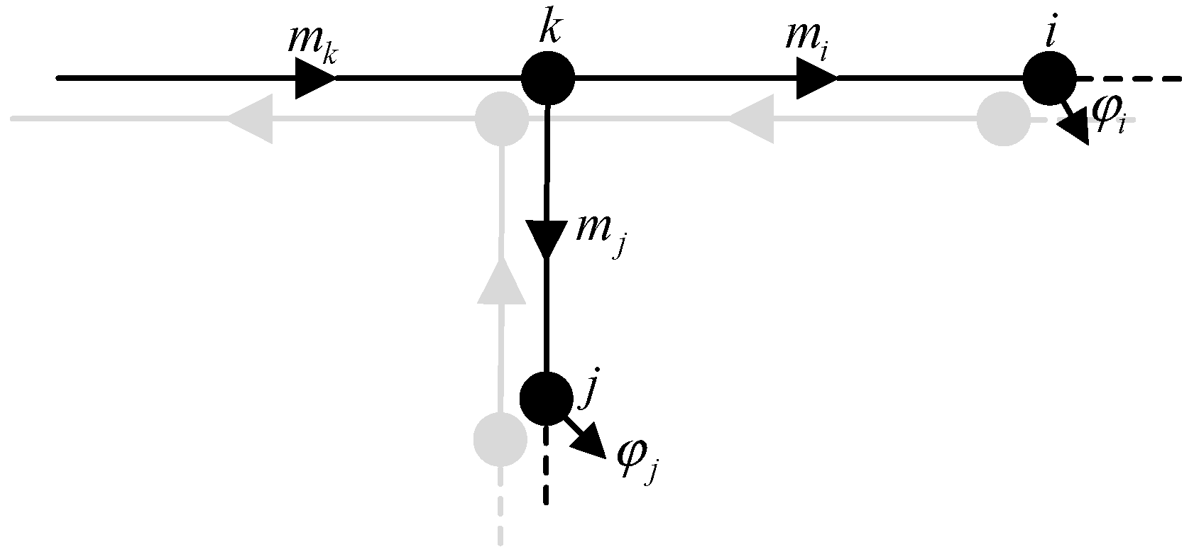
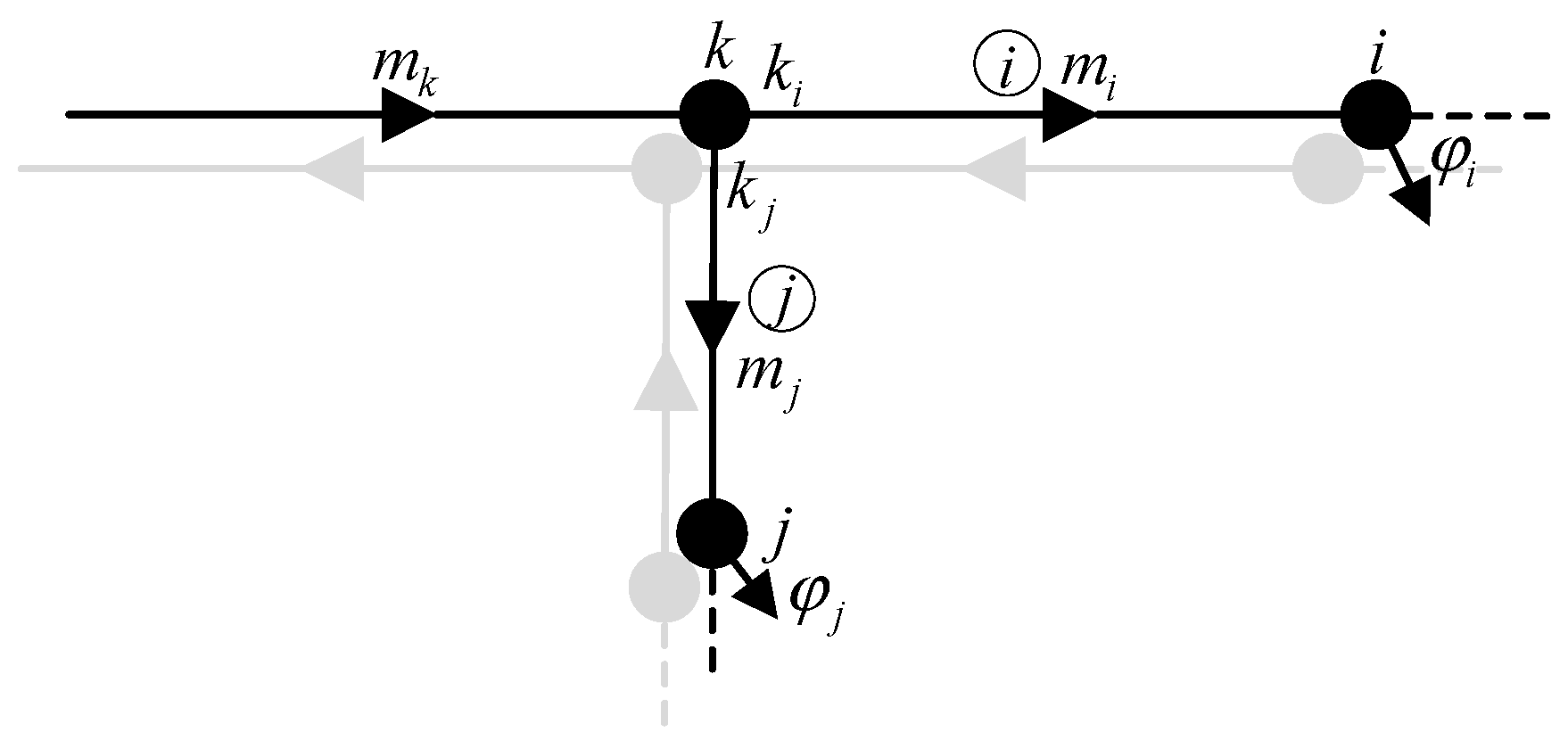
The correlation coefficient between mass flow rates can be investigated according to Lemma 3 based on the schematic presented in Figure 2. Here, the correlation coefficient between mass flow rates m_i and m_j is assumed to be ρ_ij. Because m_i and m_j originate from the same node, m_i and m_j mainly depend on the thermal energy flowing through pipes i and j. Therefore, the value of ρ_ij is very small, and the correlation coefficient between m_i and m_j can be approximated as 0. As can be seen from Lemma 4, m_i and m_j can be considered to be independent of each other. The flow balance equation for node k can be determined from Figure 2.

$$m_k=m_i+m_j.$$

(11)

Combining Equation (11) and Lemma 3 yields the following:

$${\sigma }_{m_k}^2={\sigma }_{m_i}^2+{\sigma }_{m_j}^2+2{\rho }_{ij}{\sigma }_{m_i}{\sigma }_{mj}.$$

(12)

Because ρ_ij ≈ 0, Equation (12) can be given as:

$${\sigma }_{m_k}^2={\sigma }_{m_i}^2+{\sigma }_{m_j}^2.$$

(13)

As shown in Appendix B, setting the sum of all thermal loads flowing through pipe i to ${\displaystyle \sum {\phi }_i}$ and its variance as ${\displaystyle \sum {\sigma }_{{\phi }_i}^2}$ and setting the sum of all thermal loads flowing through pipe j to ${\displaystyle \sum {\phi }_j}$ and its variance as ${\displaystyle \sum {\sigma }_{{\phi }_j}^2}$ yield the following expressions:

$${\sigma }_{m_i}^2\approx \frac{{\displaystyle \sum {\sigma }_{{\phi }_i}^2}}{{\displaystyle \sum {\sigma }_{{\phi }_i}^2}+{\displaystyle \sum {\sigma }_{{\phi }_j}^2}}{\sigma }_{m_k}^2$$

(14)

$${\sigma }_{m_j}^2\approx \frac{{\displaystyle \sum {\sigma }_{{\phi }_j}^2}}{{\displaystyle \sum {\sigma }_{{\phi }_i}^2}+{\displaystyle \sum {\sigma }_{{\phi }_j}^2}}{\sigma }_{m_k}^2.$$

(15)

Because the variance ${\sigma }_{m_1}^2$ of the mass flow through pipe 1 is known from Equation (10), the variances of the mass flow rate through pipes adjacent to pipe 1 can be obtained according to Equations (14) and (15), and the variances of mass flow rates through all other pipes in the network can be obtained in the same way. This process is generalized as follows.

If n pipes are connected to node k and the pipe indices are defined as i₁, i₂, …, i_n, then Equations (14) and (15) can be established for all mass flow rates in the pipe network as follows:

$${\sigma }_{m_{i_1}}^2\approx \frac{{\displaystyle \sum {\sigma }_{{\phi }_{i_1}}^2}}{{\displaystyle \sum {\sigma }_{{\phi }_{i_1}}^2}+{\displaystyle \sum {\sigma }_{{\phi }_{i_2}}^2}+\dots +{\displaystyle \sum {\sigma }_{{\phi }_{i_n}}^2}}{\sigma }_{m_k}^2$$

(16)

$${\sigma }_{m_{i_2}}^2\approx \frac{{\displaystyle \sum {\sigma }_{{\phi }_{i_2}}^2}}{{\displaystyle \sum {\sigma }_{{\phi }_{i_1}}^2}+{\displaystyle \sum {\sigma }_{{\phi }_{i_2}}^2}+\dots +{\displaystyle \sum {\sigma }_{{\phi }_{i_n}}^2}}{\sigma }_{m_k}^2$$

(17)

……

$${\sigma }_{m_{i_n}}^2\approx \frac{{\displaystyle \sum {\sigma }_{{\phi }_{i_n}}^2}}{{\displaystyle \sum {\sigma }_{{\phi }_{i_1}}^2}+{\displaystyle \sum {\sigma }_{{\phi }_{i_2}}^2}+\dots +{\displaystyle \sum {\sigma }_{{\phi }_{i_n}}^2}}{\sigma }_{m_k}^2.$$

(18)

Accordingly, the following equations for pipe i can be obtained:

$${\mathrm{C}}_{\mathrm{p}}{m}_i(T_{star{t}_i}-T_{en{d}_i})=\Delta {\phi }_i$$

(19)

$$\Delta {\phi }_i=h_i{L}_i(T_{star{t}_i}-T_a).$$

(20)

Here, T_starti and T_endi indicates the temperature at the start and the end of pipe i respectively. Equation (19) can be revised according to Equation (20) as follows:

$$C_p{m}_i(T_{star{t}_i}-T_{en{d}_i})=h_i{L}_i(T_{star{t}_i}-T_a),$$

(21)

which can be rewritten as:

$$T_{star{t}_i}-T_{en{d}_i}=\frac{h_i{L}_i(T_{star{t}_i}-T_a)}{{\mathrm{C}}_{\mathrm{p}}{m}_i}.$$

(22)

If the temperature of node i is T_i, the mass flow rate is from H to node i, and the pipes transmitting the mass flow rates are re-indexed as x₁, x₂, …, x_k, while the temperatures of the nodes are re-indexed as $T_{x_1}$, $T_{x_2}$, …, $T_{x_k}$. This yields the following for pipe 1 in Figure 1 (i.e., pipe x₁):

$$T_H-T_{x_1}=\frac{h_{x_1}{L}_{x_1}(T_H-T_a)}{{\mathrm{C}}_{\mathrm{p}}{m}_{x_1}},$$

(23)

while the following is obtained for the pipe 2 in Figure 1 (i.e., pipe x₂):

$$T_{x_1}-T_{x_2}=\frac{h_{x_2}{L}_{x_2}(T_{x_1}-T_a)}{{\mathrm{C}}_{\mathrm{p}}{m}_{x_2}}.$$

(24)

Similarly, this can be extended for an arbitrary pipe x_k as follows:

$$T_{x_{k-1}}-T_{x_k}=\frac{h_{x_k}{L}_{x_k}(T_{x_{k-1}}-T_a)}{{\mathrm{C}}_{\mathrm{p}}{m}_{x_k}}.$$

(25)

Adding Equations (23)–(25) yields the following:

$$T_H-T_{x_k}=\frac{h_{x_1}{L}_{x_1}(T_H-T_a)}{{\mathrm{C}}_{\mathrm{p}}{m}_{x_1}}+\frac{h_{x_2}{L}_{x_2}(T_{x_1}-T_a)}{{\mathrm{C}}_{\mathrm{p}}{m}_{x_2}}+\dots +\frac{h_{x_k}{L}_{x_k}(T_{x_{k-1}}-T_a)}{{\mathrm{C}}_{\mathrm{p}}{m}_{x_k}},$$

(26)

which can be written as:

$$T_{x_k}=T_H-\{\frac{h_{x_1}{L}_{x_1}(T_H-T_a)}{{\mathrm{C}}_{\mathrm{p}}{m}_{x_1}}+\frac{h_{x_2}{L}_{x_2}(T_{x_1}-T_a)}{{\mathrm{C}}_{\mathrm{p}}{m}_{x_2}}+\dots +\frac{h_{x_k}{L}_{x_k}(T_{x_{k-1}}-T_a)}{{\mathrm{C}}_{\mathrm{p}}{m}_{x_k}}\}.$$

(27)

Lemma 5.

Assume that a continuous random variable X has a probability density function f_x(x). It is also assume that a function y = g(x) is monotonous and its inverse function is x = g⁻¹(x). Accordingly, Y = g(X) is a continuous random variable whose probability density function is:

$$f_Y(y)=f_X[g^{-1}(y)]|\frac{d{g}^{-1}(y)}{dy}|.$$

The PDF of a random variable x = m obtained from a normal distribution is:

$$f(x)=\frac{1}{\sqrt{2\mathsf{\pi }}{\sigma }_i}{e}^{\frac{-{(x-u_i)}^2}{2{\sigma }_i^2}},$$

(28)

where u_i and σ_i² are the mean and variance, respectively. Therefore, the probability density function of y = 1/x = 1/m_i is given from Lemma 5 as follows:

$$f(y)=\frac{1}{y^2}\cdot \frac{1}{\sqrt{2\mathsf{\pi }}{\sigma }_i}{e}^{\frac{-{(\frac{1}{y}-u_i)}^2}{2{\sigma }_i^2}},$$

(29)

which can be written in the following form:

$$f(y)=\frac{1}{y^2}\cdot \frac{1}{\sqrt{2\mathsf{\pi }}{\sigma }_i}{e}^{\frac{-{(1-u_{i}y)}^2}{2{\sigma }_i^2{y}^2}}=\frac{1}{y^2}\cdot \frac{1}{\sqrt{2\mathsf{\pi }}{\sigma }_i}{e}^{-{(y-\frac{1}{u_i})}^2/(2{\sigma }_i^2{y}^2/u_i^2)}.$$

(30)

Based on the form of Equation (28), if the mean of y in Equation (30) is 1/u_i, the standard deviation is (σ_i·y)/u_i, where y = 1/u_i. As such, the standard deviation of Equation (30) is σ_i/u_i², and Equation (30) can be rewritten as follows:

$$f(y)=\frac{1}{\sqrt{2\mathsf{\pi }}({\sigma }_i/u_i^2)}{e}^{-{(y-\frac{1}{u_i})}^2/(2{\sigma }_i^2/u_i^4)}.$$

(31)

Therefore, if the mean and standard deviation of a random variable x = m_i obtained from a normal distribution are, respectively, u_i and σ_i, then y = 1/x = 1/m_i approximates a normal distribution, and its mean and standard deviation are 1/u_i and σ_i/u_i², respectively.

Similarly, as shown in Appendix C, the correlation coefficient between mass flow rate m_k and m_i in Figure 2 (ρ_ki) and the correlation coefficient between mass flow rate m_k and m_j (ρ_kj) can be obtained as follows:

$${\rho }_{ki}\approx \frac{{\sigma }_{m_i}}{\sqrt{{\sigma }_{m_i}^2+{\sigma }_{m_j}^2}}$$

(32)

$${\rho }_{kj}\approx \frac{{\sigma }_{m_j}}{\sqrt{{\sigma }_{m_i}^2+{\sigma }_{m_j}^2}}.$$

(33)

Lemma 6.

Assuming that the correlation coefficient between mass flow rate m_A and m_B for adjacent pipes A and B, respectively, is ρ_AB and the correlation coefficient between mass flow rate m_B and m_C for adjacent pipes B and C, respectively, is ρ_BC, then the correlation coefficient between m_A and m_C is ρ_AC = ρ_AB·ρ_BC if only a single unique path leads from pipe A to pipe C.

The correlation coefficients of any two mass flow rates through pipes x₁, x₂, …, x_k can be obtained from Equations (32) and (33) and Lemma 6. Accordingly, assuming that the correlation coefficient between mass flow rate passing through pipes x₁ and x₂ is ρ₁₂, and ρ₂₁ = ρ₁₂, the covariance matrix ∑ of the district heating network can be given as follows:

$${\displaystyle \sum }=\left[\begin{array}{cccc}{\sigma }_1^2& {\rho }_{12}{\sigma }_1{\sigma }_2& \cdots & {\rho }_{1n}{\sigma }_1{\sigma }_n\\ {\rho }_{21}{\sigma }_1{\sigma }_2& {\sigma }_2^2& \cdots & {\rho }_{2n}{\sigma }_2{\sigma }_n\\ ⋮& ⋮& \ddots & ⋮\\ {\rho }_{n1}{\sigma }_1{\sigma }_n& {\rho }_{n2}{\sigma }_n{\sigma }_2& & {\sigma }_n^2\end{array}\right].$$

(34)

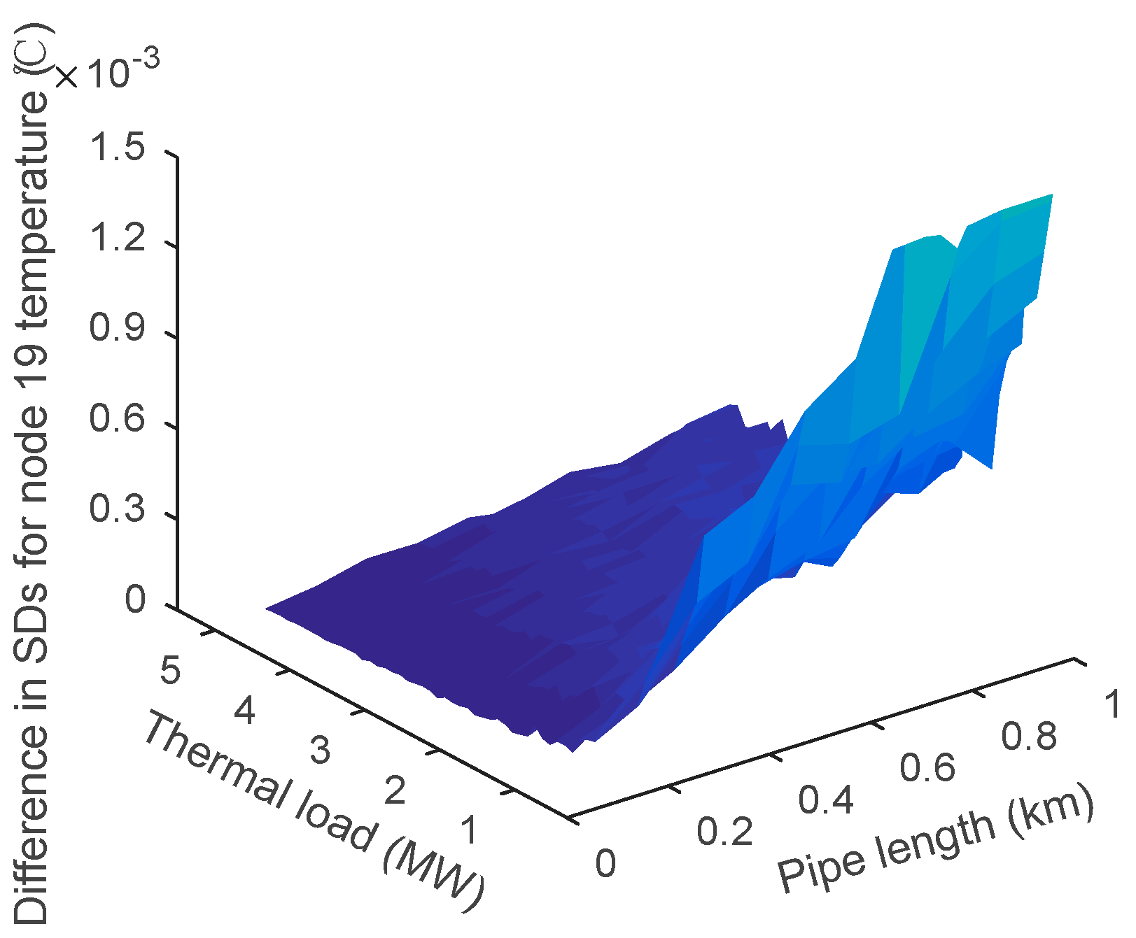
When a thermal load fluctuates, the temperature change of the corresponding node is relatively small. Then, the temperatures $T_H$, $T_{x_1}$, …, $T_{x_{k-1}}$ in Equation (27) are desirable for their mean value, where the error is small at this time and can be approximately ignored.

Lemma 7.

IfX = (X₁, X₂, …, X_n) follows the n-dimensional normal distribution N(a, B) and C is an arbitrary m × n matrix, then Y = C·X follows the m-dimensional normal distribution N(C·a, C·B·C^T), where a and B are the mathematical expectation and covariance matrix of the random variable X, respectively.

According to Lemma 7, the probability distribution of $T_{x_k}$ (or T_i) in Equation (27) can be obtained from Equations (32)–(34).

2.4. Coupling Elements between Electrical and District Heating Network

The coupling elements acting between electrical and district heating network include cogeneration CHP units, heat pumps, electric boilers, and circulating pumps. Both electrical and thermal energy are supplied by CHP units simultaneously. Heat pumps and electric boilers convert electrical energy into heat. Circulating pumps consume electrical energy to circulate water in the thermal system. These coupling components help to increase the operational flexibility of interconnected electrical-thermal IESs.

CHP units can be divided into two types, depending on whether they employ a fixed thermoelectric ratio (such as gas turbines and reciprocating internal combustion engines) or a variable thermoelectric ratio (such as exhaust steam turbines). A fixed thermoelectric ratio C_m and a variable thermoelectric ratio C_z can be obtained from the electrical energy generation P_CHP and the heat generation φ_CHP of a CHP unit as follows:

$$C_m={\mathsf{\Phi }}_{CHP}/P_{CHP}$$

(35)

$$C_z=\Delta \mathsf{\Phi }/\Delta P={\mathsf{\Phi }}_{CHP}/({\eta }_e{F}_{in}-P_{CHP}).$$

(36)

Here, η_e is the condensation efficiency, and F_in is the fuel input rate of the CHP unit.

3. Case Study

The 23-node radial district heating network shown in Figure 3 was employed for conducting a case study of the proposed nonlinear analytical algorithm for predicting the probabilistic mass flows of radial district heating network. The CHP source temperature T_H is constant at 80°C. The return water temperature T_o of the load node is constant at 45°C. The ambient temperature T_a is simplified to be a constant, which is set as 10 °C. The remaining parameters of the district heating network are presented in Appendix D.

The mean mass flow rate (μ_m), standard deviation of the mass flow rate (σ_m), mean node temperature (μ_T), and standard deviation of the node temperature (σ_T) obtained for the test system using the proposed method with those obtained using the Monte Carlo method (simulated 50,000 times) expressed as μ_m,mcs, σ_m,mcs, μ_T,mcs, and σ_T,mcs, respectively are compared. Assuming that the Monte Carlo simulation values are approximately accurate, the error in our analytical algorithm according to the absolute value differences between the two values obtained, which are represented by (|μ_m − μ_m,mcs|/μ_m,mcs) × 100% = δ_μ,m, |σ_m − σ_m,mcs| = δ_σ,m, (|μ_T − μ_T,mcs|/μ_T,mcs) × 100% = δ_μ,T, and |σ_T − σ_T,mcs| = δ_σ,T, are evaluated. Four tests were conducted. Test 1 involved setting each mean thermal load (μ_φ) to 0.5 MW with fluctuations (σ_φ) within ±10%. If this fluctuation corresponds to the 99.7% confidence level for a Gaussian distribution, then the standard deviation of each thermal load is 0.5 × 0.1/3 = 0.0167 MW. Test 1 was divided into two parts, where the first part employed L = 300 m, while the second part of the test employed L = 1000 m. Test 2 involved the same μ_φ = 0.5 MW as test 1, but with L = 1500 and a range of thermal load fluctuations within ±10%, ±20%, ±30%, and ±40%. Test 3 compared the mean and standard deviations of pipe temperature drops obtained for the test system using the proposed method, which are expressed as μ_ΔT and σ_ΔT, respectively, with those obtained using Monte Carlo (simulated 50,000 times), expressed as μ_ΔT,mcsΔ and σ_ΔT,mcs, respectively. The absolute value differences between the two values obtained are represented as (|μ_ΔT − μ_ΔT,mcs|/μ_ΔT,mcs) × 100% = δ_{μ, ΔT} and |σ_ΔT − σ_ΔT,mcs| = δ_{σ, ΔT}. Test 3 again involved setting μ_φ = 0.5 MW, as test 1, and three conditions were considered, including σ_φ = ±10% with L = 300 m, σ_φ = 50% with L = 300 m, and σ_φ = ±50% with L = 1000 m. Test 4 was divided into four parts, where the first part employed μ_φ = 1 MW, σ_φ = ±10%, and varying values of L from 100 m to 2000 m; the second part employed L = 500 m, σ_φ = ±10%, and varying μ_φ from 0.2 MW to 2.0 MW; the third part employed L = 500 m, μ_φ = 1 MW, and varying σ_φ from 0 to ±50%; and the fourth part employed σ_φ = ±10% with varying values of both L and μ_φ.

3.1. Test 1-Typical Mean and Variances of Network States

(1) For part 1 of test 1, the calculated mean and standard deviations of the mass flow rates and node temperatures for selected pipes are shown in

Table 1. Typical mean and standard deviations of mass flow rates. (Test 1: L = 300 m; μ_φ = 0.5 MW; σ_φ = ±10%).

Pipe Number	μm (kg/s)	σm (kg/s)	μm,mcs (kg/s)	σm,mcs (kg/s)	δμ,m (%)	δσ,m (kg/s)
1	41.7594	0.3944	41.7603	0.3920	0.0022	0.0024
4	27.9077	0.3232	27.9088	0.3220	0.0039	0.0012
6	6.9896	0.1616	6.9894	0.1612	0.0029	0.0004
9	6.9404	0.1616	6.9399	0.1619	0.0072	0.0003
10	3.4714	0.1143	3.4710	0.1146	0.0115	0.0003
13	6.9674	0.1616	6.9677	0.1617	0.0043	0.0001
14	3.4858	0.1143	3.4857	0.1144	0.0029	0.0001
17	10.4813	0.1979	10.4824	0.1977	0.0105	0.0002
19	3.4981	0.1143	3.4993	0.1152	0.0343	0.0009

and

Table 2. Typical mean and standard deviations of node temperature. (Test 1: L = 300 m; μ_φ = 0.5 MW; σ_φ = ±10%).

Node Number	μT (°C)	σT (°C)	μT,mcs (°C)	σT,mcs (°C)	δμ,T (%)	δσ,T (°C)
1	79.9614	0.0004	79.9614	0.0004	0.0000	0.0000
4	79.8111	0.0019	79.8111	0.0019	0.0000	0.0000
6	79.5657	0.0058	79.5656	0.0059	0.0001	0.0001
9	79.7678	0.0039	79.7677	0.0039	0.0001	0.0000
10	79.4413	0.0138	79.4408	0.0138	0.0006	0.0000
13	79.6116	0.0058	79.6115	0.0058	0.0001	0.0000
14	79.2986	0.0148	79.2981	0.0148	0.0006	0.0000
17	79.6442	0.0040	79.6442	0.0041	0.0001	0.0001
19	79.1776	0.0148	79.1772	0.0153	0.0004	0.0005

, respectively, along with the differences between the values.

(2) For part 2 of test 1, the calculated mean and standard deviations of the mass flow rates and temperature for selected pipes are shown in

Table 3. Typical mean and standard deviations of mass flow rates. (Test 1: L = 1000 m; μ_φ = 0.5 MW; σ_φ = ±10%).

Pipe Number	μm (kg/s)	σm (kg/s)	μm,mcs (kg/s)	σm,mcs (kg/s)	δμ,m (%)	δσ,m (kg/s)
1	43.5224	0.3944	43.5218	0.3945	0.0015	0.0001
4	29.2376	0.3232	29.2357	0.3219	0.0066	0.0013
6	7.3506	0.1616	7.3499	0.1645	0.0096	0.0030
9	7.1903	0.1616	7.1909	0.1622	0.0081	0.0006
10	3.5991	0.1143	3.5992	0.1152	0.0009	0.0010
13	7.2785	0.1616	7.2777	0.1635	0.0112	0.0019
14	3.6462	0.1143	3.6458	0.1169	0.0105	0.0027
17	11.0159	0.1979	11.0150	0.2016	0.0079	0.0037
19	3.6862	0.1143	3.6859	0.1184	0.0084	0.0041

and

Table 4. Typical mean and standard deviations of node temperature. (Test 1: L = 1000 m; μ_φ = 0.5 MW; σ_φ = ±10%).

Node Number	μT (°C)	σT (°C)	μT,mcs (°C)	σT,mcs (°C)	δμ,T (%)	δσ,T (°C)
1	79.8767	0.0011	79.8766	0.0011	0.0000	0.0000
4	79.3994	0.0058	79.3993	0.0058	0.0001	0.0001
6	78.6283	0.0173	78.6279	0.0178	0.0006	0.0005
9	79.2573	0.0121	79.2571	0.0121	0.0003	0.0000
10	78.2206	0.0425	78.2194	0.0422	0.0016	0.0003
13	78.7685	0.0176	78.7680	0.0176	0.0006	0.0001
14	77.7879	0.0448	77.7863	0.0449	0.0020	0.0000
17	78.8741	0.0120	78.8738	0.0124	0.0003	0.0004
19	77.4259	0.0437	77.4244	0.0458	0.0019	0.0021

, respectively, along with the differences between the values.

It can be noted from Table 1 and Table 3 that increasing the value of L from 300 m to 1000 m, while holding the mean thermal loads and fluctuations constant, increased both the mean mass flow rates error and the mass flow rates standard deviation error. Nonetheless, the maximum error in the mean mass flow rate was less than 0.03%, while the maximum error in the standard deviation of the mass flow rate was less than 0.004 kg/s. Table 2 and Table 4 indicate that similar results were obtained for the mean temperature error and the temperature standard deviation error, where both increased with increasing L, although the maximum mean temperature error was less than 0.002%, while the maximum temperature standard deviation error was less than 0.002 °C.

3.2. Test 2-Typical Mean and Variances of Network States

For test 2, the calculated mean and standard deviations of the mass flow rate and temperature for selected pipes are shown in

Table 5. Typical mean and standard deviations of mass flow rates. (Test 2: L = 1500 m; μ_φ = 0.5 MW).

Thermal Load Fluctuation	Pipe NO.	μm (kg/s)	σm (kg/s)	μm,mcs (kg/s)	σm,mcs (kg/s)	δμ,m (%)	δσ,m (kg/s)
Within 10%	1	44.7603	0.3944	44.7619	0.3962	0.0037	0.0017
	4	30.1700	0.3232	30.1701	0.3252	0.0001	0.0020
	6	7.6035	0.1616	7.6041	0.1652	0.0082	0.0036
	19	3.8179	0.1143	3.8181	0.1200	0.0058	0.0058
Within 20%	1	44.7603	0.7889	44.7641	0.7866	0.0084	0.0023
	4	30.1700	0.6464	30.1713	0.6467	0.0042	0.0004
	6	7.6035	0.3232	7.6055	0.3328	0.0260	0.0096
	19	3.8179	0.2285	3.8180	0.2412	0.0036	0.0127
Within 30%	1	44.7603	1.1833	44.7514	1.1921	0.0198	0.0087
	4	30.1700	0.9696	30.1628	0.9737	0.0240	0.0041
	6	7.6035	0.4848	7.6054	0.4961	0.0255	0.0113
	19	3.8179	0.3428	3.8176	0.3618	0.0068	0.0190
Within 40%	1	44.7603	1.5778	44.7499	1.5876	0.0231	0.0098
	4	30.1700	1.2928	30.1597	1.2960	0.0343	0.0032
	6	7.6035	0.6464	7.6020	0.6644	0.0196	0.0181
	19	3.8179	0.4571	3.8173	0.4836	0.0139	0.0266

and

Table 6. Typical mean and standard deviations of node temperature. (Test 2: L = 1500 m; μ_φ = 0.5 MW).

Thermal Load Fluctuation	Node NO.	μT (°C)	σT (°C)	μT,mcs (°C)	σT,mcs (°C)	δμ,T (%)	δσ,T (°C)
Within ±10%	1	79.8202	0.0016	79.8202	0.0016	0.0000	0.0000
	4	79.1274	0.0082	79.1273	0.0082	0.0001	0.0000
	6	78.0158	0.0242	78.0154	0.0249	0.0005	0.0007
	19	76.2980	0.0606	76.2963	0.0634	0.0023	0.0028
Within ±20%	1	79.8202	0.0032	79.8201	0.0032	0.0001	0.0000
	4	79.1274	0.0165	79.1271	0.0163	0.0003	0.0002
	6	78.0158	0.0484	78.0141	0.0501	0.0021	0.0017
	19	76.2980	0.1212	76.2911	0.1284	0.0092	0.0072
Within ±30%	1	79.8202	0.0048	79.8200	0.0048	0.0002	0.0000
	4	79.1274	0.0247	79.1264	0.0247	0.0012	0.0000
	6	78.0158	0.0725	78.0113	0.0754	0.0057	0.0029
	19	76.2980	0.1818	76.2807	0.1956	0.0227	0.0138
Within ±40%	1	79.8202	0.0063	79.8199	0.0064	0.0003	0.0001
	4	79.1274	0.0330	79.1258	0.0330	0.0020	0.0000
	6	78.0158	0.0967	78.0072	0.1018	0.0110	0.0051
	19	76.2980	0.2424	76.2669	0.2676	0.0408	0.0252

, respectively, along with the differences between the values.

In addition, Figure 4a–d present the cumulative density functions (CDFs) of mass flow rate through pipe 1 and node 19 temperature under thermal load fluctuations within 10%, 20%, 30%, and 40%, respectively.

It can be noted from Table 5 and Table 6 that increasing the thermal load fluctuation with constant L and μ_φ increased the standard deviations of the mass flow rates and the temperature. Nevertheless, for thermal load fluctuations of 10%, 20%, 30%, and 40%, the maximum errors in the mass flow rates standard deviation were 0.0058 kg/s, 0.0127 kg/s, 0.0190 kg/s, and 0.0266 kg/s, respectively, while the maximum errors in the node temperature standard deviation were 0.0028 °C, 0.0072 °C, 0.0138 °C, and 0.0252 °C, respectively. In addition, it can be noted that the mean values of the mass flow rates and the node temperature obtained by the Monte Carlo method decreased with increasing thermal load fluctuation.

3.3. Test 3-Probability Density Function of Pipeline Temperature Drops

For test 3, the calculated mean and standard deviations of the pipe temperature drops obtained for selected pipes are shown in

Table 7. Typical mean and standard deviations of pipe temperature drops. (Test 3: μ_φ = 0.5 MW).

Pipe Length (L; m)	Thermal Load Fluctuation (φ)	Pipe NO.	μΔT (°C)	σΔT (°C)	μΔT,mcs (°C)	σΔT,mcs (°C)	δμ, ΔT (%)	δσ, ΔT (°C)
300	Within ±10%	1	0.0386	0.0004	0.0386	0.0004	0.0215	0.0000
		2	0.0421	0.0004	0.0420	0.0004	0.0214	0.0000
		3	0.0496	0.0005	0.0496	0.0005	0.0230	0.0000
		4	0.0587	0.0007	0.0587	0.0007	0.0261	0.0000
		5	0.0768	0.0010	0.0767	0.0010	0.0356	0.0000
300	Within ±50%	1	0.0386	0.0018	0.0387	0.0018	0.1988	0.0000
		2	0.0421	0.0021	0.0421	0.0021	0.2192	0.0000
		3	0.0496	0.0027	0.0497	0.0027	0.2782	0.0000
		4	0.0587	0.0034	0.0589	0.0034	0.3179	0.0000
		5	0.0768	0.0051	0.0771	0.0052	0.4138	0.0001
1000	Within ±50%	1	0.1235	0.0056	0.1236	0.0056	0.0939	0.0000
		2	0.1341	0.0064	0.1342	0.0063	0.0954	0.0000
		3	0.1576	0.0082	0.1578	0.0082	0.1242	0.0000
		4	0.1861	0.0103	0.1864	0.0103	0.1465	0.0000
		5	0.2426	0.0155	0.2430	0.0157	0.1901	0.0002

along with the differences between the values.

It can be seen from Table 7 that increasing the thermal load fluctuation with constant L and μ_φ increased the mean pipe temperature drop obtained by Monte Carlo simulations slightly. Meanwhile, increasing the thermal load fluctuation by a factor of 5 with a constant L increased the standard deviation of the pipe temperature drop obtained by Monte Carlo simulations by a factor of 5 generally, and increasing L by a factor of 3 and 1/3 with a constant σ_φ increased both the mean and standard deviations of pipe temperature drops by a factor a little less than 3 and 1/3.

3.4. Test 4-Control Variable Method

(1) From Table 2, It can be noted that the value of σ_T,mcs is greatest for node 19. Therefore, the value σ_T,mcs for node 19 with constants μ_φ and σ_φ while varying L is determined, and the results are shown in Figure 5. It can be seen from the figure that the value of σ_T,mcs for node 19 increases approximately linearly with increasing L.

(2) The value σ_T,mcs for node 19 with constants L and σ_φ while varying μ_φ, is also determined and the results are shown in Figure 6. It can be seen from the figure that the value of σ_T,mcs for node 19 decreases nonlinearly as μ_φ increases, and approaches zero asymptotically.

(3) The value σ_T,mcs for node 19 with constants L and μ_φ while varying σ_φ, is also determined and the results are shown in Figure 7. It can be seen from the figure that the value of σ_T,mcs for node 19 increases approximately linearly with increasing σ_φ. Nonetheless, the value of σ_T,mcs for node 19 remains small even at large σ_φ.

(4) The value σ_m,mcs for pipe 1 with constant σ_φ while varying both L and μ_φ, is also determined and the results are shown in Figure 8. It can be seen from the figure that the value of L has little influence on the value of σ_m,mcs for pipe 1, and σ_m,mcs is essentially unchanged while varying L at any constant value of μ_φ. In contrast, the value of μ_φ has a significant effect on σ_m,mcs for pipe 1, and σ_m,mcs increases approximately linearly with increasing μ_φ.

(5) The value σ_T,mcs for node 19 with constant σ_φ while varying both L and μ_φ, is also determined and the results are shown in Figure 9. As can be seen from the figure, the value of σ_T,mcs for node 19 is dependent on both L and μ_φ and increases with increasing L and decreasing μ_φ. Here, L has a small effect on σ_T,mcs at high μ_φ, but the effect of L is quite significant at low μ_φ, and σ_T,mcs increases markedly with increasing L.

3.5. Model Error Analysis

The values of σ_m, σ_m,mcs, and δ_σ,m for pipe 1 and the values of σ_T, σ_T,mcs, and δ_σ,T for node 19 were compared at a constant value of σ_φ = ±10% while varying both L and μ_φ.

(1) When given values of μ_φ with L varied from 100 m to 2000 m in increments of 100 m, 20 sets standard deviation by Monte Carlo and the proposed method respectively can be get, whose average are σ_m and σ_m,mcs and the results are shown in

Table 8. Standard deviations of mass flow rate through pipe 1 under different average thermal loads μ_φ (σ_φ = ±10%).

φ (MW)	σm (kg/s)	σm,mcs (kg/s)	δσ,m (%)	φ (MW)	σm (kg/s)	σm,mcs (kg/s)	δσ,m (%)
0.5	0.3944	0.3949	0.1266	2.8	2.2089	2.2359	1.2076
0.6	0.4733	0.4701	0.6807	2.9	2.2878	2.2839	0.1708
0.7	0.5522	0.5564	0.7549	3.0	2.3667	2.3954	1.1981
0.8	0.6311	0.6321	0.1582	3.1	2.4456	2.4448	0.0327
0.9	0.7100	0.7132	0.4487	3.2	2.5245	2.5287	0.1661
1.0	0.7889	0.7839	0.6378	3.3	2.6033	2.6222	0.7208
1.1	0.8678	0.8676	0.0231	3.4	2.6822	2.6708	0.4268
1.2	0.9467	0.9436	0.3285	3.5	2.7611	2.7476	0.4913
1.3	1.0256	1.0319	0.6105	3.6	2.8400	2.8294	0.3746
1.4	1.1044	1.1098	0.4866	3.7	2.9189	2.9274	0.2904
1.5	1.1833	1.1752	0.6892	3.8	2.9978	3.0175	0.6529
1.6	1.2622	1.2500	0.9760	3.9	3.0767	3.0969	0.6523
1.7	1.3411	1.3391	0.1494	4.0	3.1556	3.1442	0.3626
1.8	1.4200	1.4140	0.4243	4.1	3.2345	3.2402	0.1759
1.9	1.4989	1.4980	0.0601	4.2	3.3133	3.3300	0.5015
2.0	1.5778	1.5812	0.2150	4.3	3.3922	3.4056	0.3935
2.1	1.6567	1.6523	0.2663	4.4	3.4711	3.4549	0.4689
2.2	1.7356	1.7333	0.1327	4.5	3.5500	3.5608	0.3033
2.3	1.8145	1.8155	0.0551	4.6	3.6289	3.6131	0.4373
2.4	1.8933	1.8931	0.0106	4.7	3.7078	3.7058	0.0540
2.5	1.9722	1.9749	0.1367	4.8	3.7867	3.7793	0.1958
2.6	2.0511	2.0418	0.4555	4.9	3.8656	3.8458	0.5148
2.7	2.1300	2.1310	0.0469	5.0	3.9445	3.9694	0.6273

. It can be seen from the table that L has little influence on the standard deviation of pipe 1 mass flow rate under constants μ_φ and σ_φ and that the values of σ_m and σ_m,mcs for pipe 1 increase approximately linearly which are shown in Figure 10.

(2) Figure 11 presents the values δ_σ,T for node 19 with constant σ_φ while varying both L and μ_φ. It can be seen from the figure that the error of the proposed model increases with increasing L and decreasing μ_φ, but the value of δ_σ,T for node 19 is typically less than 0.0003°C, so the error of the proposed model is generally within an acceptable range.

4. Conclusions

This paper developed a nonlinear analytical algorithm for predicting the probabilistic mass flow of a radial district heating network based on the principle of heat transfer and basic pipe network theory. The validity and rationality of the proposed algorithm was verified by application to a 23-node radial district heating network with various pipe lengths under thermal load fluctuations of various magnitudes. The characteristics of the algorithm and the conclusions obtained are given as follows:

(1) The proposed algorithm utilizes a nonlinear mass flow model with several reasonable approximations. Consequently, the obtained operating conditions are sufficiently accurate.

(2) The algorithm provides probabilistic operational information for district heating network with stochastic heat loads. The algorithm not only provides the variances of the mass flow rate through a pipe network and the node temperatures but also obtains the variances of the pipe temperature drops.

(3) The computation is efficient because the probabilistic district heating network mass flow model is relatively simple, and our approach does not require repeated nonlinear mass flow calculations.

(4) The case study results indicate that the pipe length has little effect on the standard deviations of mass flow rates, while the mean thermal load significantly influences the standard deviations of mass flow rates.

The algorithm proposed in this paper is expected to be very useful for the calculation of district heating network probability and for conducting risk analysis.

References

1. Wu, J.; Yan, J.; Jia, H.; Hatziargyriou, N.; Djilali, N.; Sun, H. Integrated Energy Systems. J. Appl. Energy 2016, 167, 155–157. [Google Scholar] [CrossRef]
2. Omalley, M.; Kroposki, B. Energy comes together: The integrated of all systems. IEEE Power Energy Mag. 2013, 11, 18–23. [Google Scholar] [CrossRef]
3. Geidl, M.; Andersson, G. Optimal power flow of multiple energy carriers. IEEE Trans. Power Syst. 2007, 22, 145–155. [Google Scholar] [CrossRef]
4. Liu, X.Z. Combined Analysis of Electricity and Heat Networks. Ph.D. Thesis, Cardiff University, Wales, UK, 2013. [Google Scholar]
5. Liu, X.Z.; Wu, J.Z.; Jenkins, N.; Bagdanavicius, A. Combined analysis of electricity and heat networks. Appl. Energy 2016, 162, 1238–1250. [Google Scholar] [CrossRef]
6. Li, Q.; An, S.; Gedra, T.W. Solving natural gas loadflow problems using electric loadflow techniques. In Proceedings of the North American power symposium, Rolla, MO, USA, 22–25 September 2013. [Google Scholar]
7. Martinez-Mares, A.; Fuerte-Esquivel, C.R. A unified gas and power flow analysis in natural gas and electricity coupled networks. IEEE Trans. Power Syst. 2012, 27, 2156–2166. [Google Scholar] [CrossRef]
8. Shabanpour-Haghighi, A.; Seifi, A.R. An integrated steady-state operation assessment of electrical, natural gas and district heating networks. IEEE Trans. Power Syst. 2016, 31, 3636–3647. [Google Scholar] [CrossRef]
9. Wang, Y.R.; Zeng, B.; Guo, J.; Shi, J.Q.; Zhang, J.H. Multi-energy flow calculation method for integrated energy system containing electricity, heat and gas. Power Syst. Technol. 2016, 40, 2942–2950. [Google Scholar]
10. Liu, X.Z.; Mancarella, P. Modelling, assessment and Sankey diagrams of integrated electricity-heat-gas networks in multi-vector district energy systems. Appl. Energy 2016, 167, 336–352. [Google Scholar] [CrossRef]
11. Soroudi, A.; Amraee, T. Decision making under uncertainty in energy systems: State of the art. J. Renew. Sustain. Energy Rev. 2013, 28, 376–384. [Google Scholar] [CrossRef]
12. Ma, Z.; Chen, H.; Chai, Y.L. Analysis of voltage stability uncertainty using stochastic response surface method related to wind farm correlation. Prot. Control Mod. Power Syst. 2017, 2, 211–219. [Google Scholar] [CrossRef]
13. Yang, Y.; Song, A.; Liu, H. Parallel computing of multi-contingency optimal power flow with transient stability constraints. Prot. Control Mod. Power Syst. 2018, 3, 1–10. [Google Scholar] [CrossRef]
14. Chen, S.; Wei, Z.N.; Sun, G.Q.; Cheung, K.W.; Sun, Y.H. Multi-linear probabilistic energy flow analysis of integrated electrical and natural-gas systems. IEEE Trans. Power Syst. 2017, 32, 1970–1979. [Google Scholar] [CrossRef]
15. Chaudry, M.; Wu, J.Z.; Jenkins, N. A sequential Monte Carlo model of the combined GB gas and electricity network. J. Energy Policy 2013, 62, 473–483. [Google Scholar] [CrossRef]
16. Yang, L.; Zhao, X.; Li, X.; Yan, W. Probabilistic Steady-State Operation and Interaction Analysis of Integrated Electricity, Gas and Heating Systems. Energies 2018, 11, 917. [Google Scholar] [CrossRef]
17. Zhang, Y.; He, Y.; Yan, M.; Guo, C.; Ding, Y.; Zhang, Y.; He, Y.; Yan, M.; Guo, C.; Ding, Y. Linearized Stochastic Scheduling of Interconnected Energy Hubs Considering Integrated Demand Response and Wind Uncertainty. Energies 2018, 11, 2448. [Google Scholar] [CrossRef]
18. Cai, D.; Shi, D.; Chen, J. Probabilistic load flow computation with polynomial normal transformation and Latin hypercube sampling. IET Gener. Transm. Distrib. 2013, 7, 474–482. [Google Scholar] [CrossRef]
19. Hajian, M.; Rosehart, W.D.; Zareipour, H. Probabilistic power flow by Monte Carlo simulation with Latin supercube sampling. IEEE Trans. Power Syst. 2013, 28, 1550–1559. [Google Scholar] [CrossRef]
20. Zhang, P.; Lee, S.T. Probabilistic load flow computation using the method of combined Cumulants and Gram-Charlier expansion. IEEE Trans. Power Syst. 2004, 19, 676–682. [Google Scholar]
21. Schellenberg, A.; Rosehart, W.; Aguado, J. Cumulant-based probabilistic optimal power flow (P-OPF) with Gaussian and gamma distributions. IEEE Trans. Power Syst. 2005, 20, 773–781. [Google Scholar]
22. Hong, H.P. An efficient point estimate method for probabilistic analysis. Reliab. Eng. Syst. Safety 1998, 59, 261–267. [Google Scholar] [CrossRef]
23. Su, C.-L. Probabilistic load-flow computation using point estimate method. IEEE Trans. Power Syst. 2005, 20, 1843–1851. [Google Scholar] [CrossRef]
24. Soleimanpour, N.; Mohammadi, M. Probabilistic load flow by using nonparametric density estimators. IEEE Trans. Power Syst. 2013, 28, 3747–3755. [Google Scholar] [CrossRef]
Figure 1. Probabilistic mass flow model of a radial district heating network consisting of a heat source node H, three pipes, and three nodes. Here, the circled values represent pipes and the arrows represent the direction of mass flow rates.
Energies 12 01215 g001
Figure 2. Illustration describing the calculation of the mass flow rates correlation coefficient.
Energies 12 01215 g002
Figure 3. System diagram of the 23-node heat distribution network employed as a case study.
Energies 12 01215 g003
Figure 4. Cumulative density functions (CDFs) of mass flow rate through pipe 1 and node 19 temperature (Test 2: L = 1500 m; μφ = 0.5 MW) under different thermal load fluctuations: (a) within ±10%; (b) within ±20%; (c) within ±30%; and (d) within ±40%.
Energies 12 01215 g004
Figure 5. Relationship between the node temperature standard deviation of node 19 and pipe length (Test 4: μφ = 1.0 MW; σφ = ±10%).
Energies 12 01215 g005
Figure 6. Relationship between the node temperature standard deviation of node 19 and mean thermal load (Test 4: L = 500 m; σφ = ±10%).
Energies 12 01215 g006
Figure 7. Relationship between the node temperature standard deviation of node 19 and thermal load fluctuation (Test 4: L = 500 m; μφ = 1.0 MW).
Energies 12 01215 g007
Figure 8. Relationship between the standard deviation of mass flow rate for pipe 1 with respect to pipe length and mean thermal load (Test 4: σφ = ±10%).
Energies 12 01215 g008
Figure 9. Relationship between the node temperature standard deviation of node 19 with respect to pipe length and mean thermal load (Test 4: σφ = ±10%).
Energies 12 01215 g009
Figure 10. The standard deviations of mass flow rate through pipe 1 using the Monte Carlo method and the proposed analytical method with respect to average thermal load (σφ = ±10%).
Energies 12 01215 g010
Figure 11. Relationship between the differences in the standard deviations obtained for the node temperature of node 19 using the Monte Carlo method and the proposed analytical method with respect to pipe length and average thermal load (σφ = ±10%).
Energies 12 01215 g011