1. Introduction
Wind energy is a fast growing source of renewable energy. In the last decades, strong motivation for its further development has also been given by the goals established by both the European Union and the United States in order to increase the portion of electricity generated from renewable sources. As a result, research about wind energy has experienced a noticeable boost [
1,
2].
In terms of numerical modelling, a large number of complexities is involved when the aerodynamics of modern wind rotors are investigated. The growing dimensions of the rotors of horizontal axis wind turbines [
3] are increasing the complexity even further. The high Reynolds number (up to 10
8) and the atmospheric turbulence are challenging to simulate. The rotation of the moving parts and the presence of the supporting static structures of the machine (i.e., tower and nacelle) make the problem even harder to tackle and not representable by means of steady-state analysis. Moreover, wind turbines normally operate in the atmospheric boundary layer (ABL), namely a wind velocity increasing with height. This leads to the need to dynamically simulate the complete rotor, with the loads exerted on the blades oscillating in time. This interaction between the ABL and horizontal axis wind turbines was investigated by Calaf, Meneveau, and Meyers by means of large eddy simulations of wind farms. Their work highlighted a close relation between the wind shear and the power extraction [
4,
5].
However, only a limited number of works take into account the effect of the ABL or the presence of supporting structures on the aerodynamics and power production of the single turbine, whereas traditional and widely used blade element momentum (BEM) theory [
6] normally neglects these effects and limits the study to steady or quasi-steady state analysis. Furthermore, a tip-loss correction factor is needed for BEM theory to account for rotors with a finite number of blades instead of an actuator disk. A first correction was derived by Prandtl [
7] and introduced by Glauert in the BEM technique [
8]. More recently, Shen et al. [
9] reviewed various tip loss corrections proposed over the years and highlighted how they fail to correctly predict the physical behavior in the proximity of the tip, also proposing a novel method to more accurately model the flow in this region. Moreover, the capability of a BEM code to account for the presence of the ABL or supporting structures is still very limited. This is reported only in the work of Dai et al. [
10], who combined traditional BEM theory with a dynamic stall model, carrying out computations in which the ABL and the tower dam effect (i.e., the increase in pressure on the suction side of the blades due to their passage in front of the supporting tower) were accounted for.
Even though BEM provides a reasonable solution, the level of detail in the obtained results can certainly be improved. Sorensen and Kock [
11] proposed an unsteady model for horizontal axis wind turbines, based on a general actuator disk concept and using a constant inlet wind speed. Xin Shen et al. [
12] used an advanced lifting surface model to mimic the aerodynamics of the blade and also accounted for a sheared inlet wind velocity. Increasing the computational cost, Seydel and Aliseda [
13] performed numerical simulations using a Reynolds-average Navier-Stokes (RANS) turbulence model (k-ω SST) in combination with a sliding interface approach to handle the relative rotation of the analyzed wind rotor; the ABL was approximated by a piece-wise linear wind velocity distribution. Similarly, Cai et al. [
14] adopted a RANS model, coupled with a sliding interface technique, to simulate the dynamics of a wind turbine with supporting structures immersed in the ABL, reproducing the wind velocity by a power law. All the works by Shen et al., by Seydel and Aliseda, and by Cai et al. reported sinusoidal loadings acting on the blades as a consequence of wind velocity stratification, highlighting the importance of the ABL in the simulations of modern wind turbines.
In the first part, this work will focus on the effect of the ABL and the presence of the supporting structures on the operation of a large (100 m diameter) commercial horizontal axis wind turbine, both in terms of performance and blade loading. A RANS turbulence model will be used, in combination with appropriate boundary conditions and modified wall functions, specifically adopted to ensure that the imposed ABL is preserved.
Additionally, a noticeable amount of research is currently being performed on the effect of rotor misalignment with respect to the incoming wind. However, most of the literature focuses on tilt and yaw misalignment as wake redirection techniques in wind farms, with the final goal of enhancing the global power production by letting every machine work outside the wakes of its neighbors. Fleming et al. [
15] carried out a large quantity of large-eddy simulations (LES) with the objective of using the tilt angle and yaw misalignment (as well as turbine repositioning) of two turbines in a row to maximize their output power. Annoni et al. [
16] performed a similar numerical investigation on a sole rotor tilting as a wake redirection technique and its effectiveness as a power gain strategy in wind farms. Noura et al. [
17] used delayed detached eddy simulations (DDES) in combination with sliding interfaces to investigate the effect of a yaw misalignment on the wake of a small wind turbine, neglecting both the supporting structures and the ABL. Also, some experimental works on simplified small scale wind turbine models [
18] or on full scale commercial turbines [
19] have been carried out in order to maximize the power output.
Even though the current research focuses on rotor misalignment as a wake redirection technique in wind farms, every large horizontal axis wind turbine (HAWT) operates under tilted and yawed conditions. A small tilt is always imposed on the rotor and nacelle to provide the blades with more clearance from the tower, reduce the tower dam effect, and prevent collision due to large deflections. Additionally, LIDAR (light imaging, detection, and ranging) field measurements on large HAWTs have shown that, during normal operation, a yaw misalignment of 4 to 10 degrees is due to uncertainty in the wind direction measurement [
20].
For these reasons, in the current work, the considered machine (always immersed in the ABL and in the presence of the supporting structures) is also simulated under tilted and tilted-yawed conditions, comparing the results with the untilted and unyawed configuration. A particular focus will be placed on investigating the aerodynamics of each blade, analyzing the effect of the imposed misalignments on their energy conversion performance as well as on the load acting on them. This represents the main novelty of the present work, compared to the works currently present in the literature and focusing on the effect of misalignments on the global power production of wind farms.
The details of the employed numerical model are given in
Section 2, while the results of the performed simulations are discussed in
Section 3. In that section, the results of the rotor-only and full-machine simulations are covered first, before analyzing the effect of tilt and yaw separately. Lastly, conclusions are drawn in
Section 4.
2. Methodology
2.1. Layout, Mesh, and Overset Approach
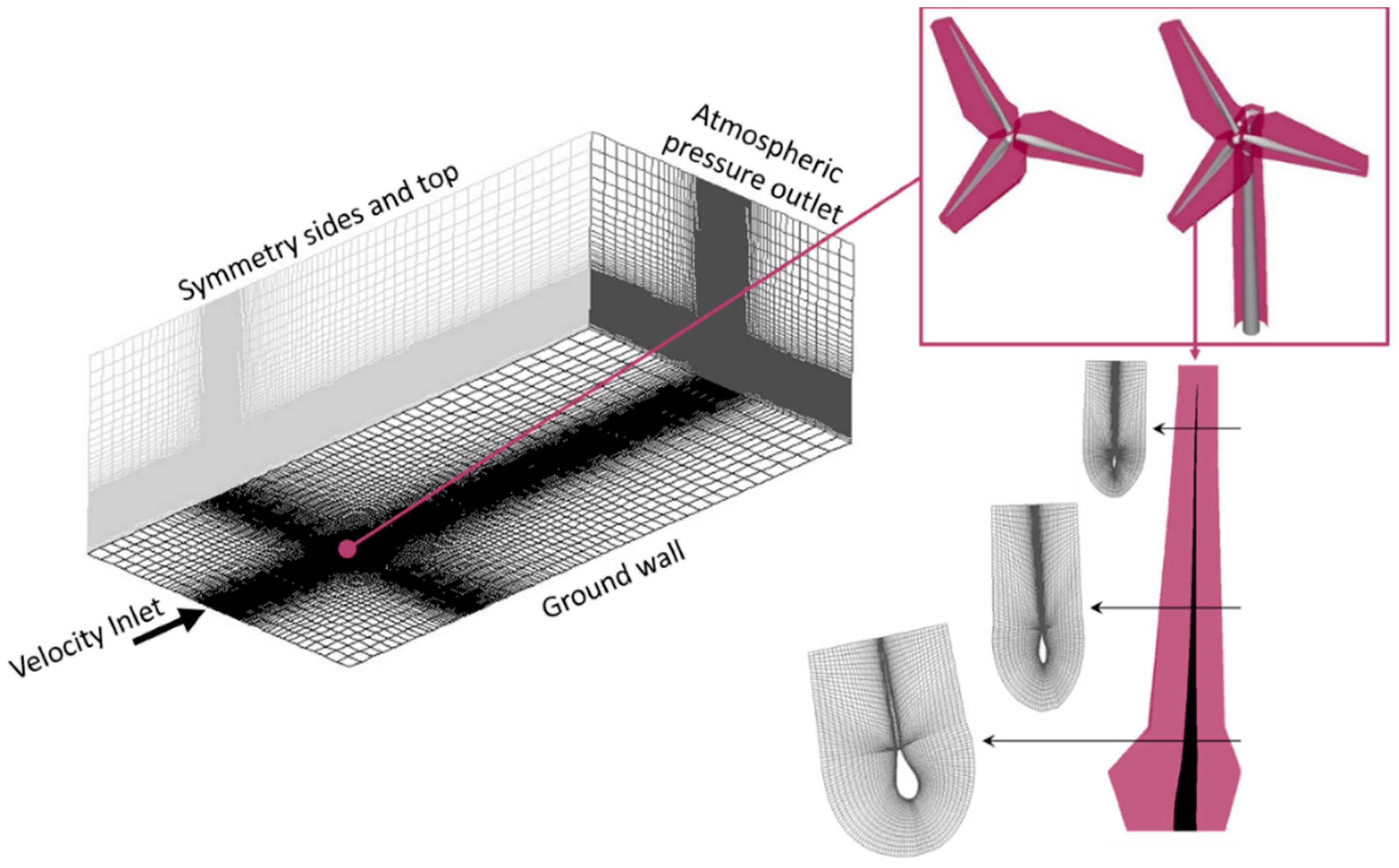
The layout of the employed model is shown in
Figure 1, together with the implemented boundary conditions and the details of the used meshes.
The geometry of the rotor and supporting structures (only in the full machine simulations) is modelled. The diameter of the rotor measures 100 m and the machine is placed as shown in
Figure 1. The inlet and the pressure outlet (where the pressure is set to 1 atm) are placed, respectively, 5 and 15 rotor diameters away from the rotor. The symmetry side and top surfaces (on which no orthogonal flow is allowed) are also positioned at a distance of 5 rotor diameters from the turbine location. These distances are chosen according to good practice guidelines for atmospheric flows [
21] in order to avoid any artificial influence of the boundaries on the flow in the proximity of the turbine. Nevertheless, approximately half of these distances are adopted in similar computational fluid dynamics (CFD) works [
14,
22] and were found to be sufficient to minimize any boundary influence [
23].
A three-dimensional component mesh for the overset technique is generated around every object to be simulated, namely the three blades, the hub of the machine, and (for the full machine simulations) its supporting structures (tower and nacelle), as shown in
Figure 1—right. The tower geometry is selected to be suitable for machines of this size and is extracted from [
24], with a height of 100 m. The nacelle is 12 m long and its section measures 5 m × 5 m. The mesh on each blade wall is designed to ensure a
in the log layer (between 30 and 300). The mesh size is then increased away from the wall in order to be comparable to the mesh size (0.275 m) of the structured background grid (
Figure 1—left) at the boundary of each component mesh.
Figure 1—right shows several sections of the fluid mesh around each blade, highlighting the C-grid adopted for its generation and the tapering and twisting of the blades, followed by the created mesh. The total number of cells in the computational domain is approximately 55 million, of which 1.9 million belong to each blade component mesh. In total, 38,500 faces are distributed on the surface of each blade. The mesh size is chosen according to previous studies performed by the authors [
25]. All these meshes mutually overlay and are connected by means of an overset technique.
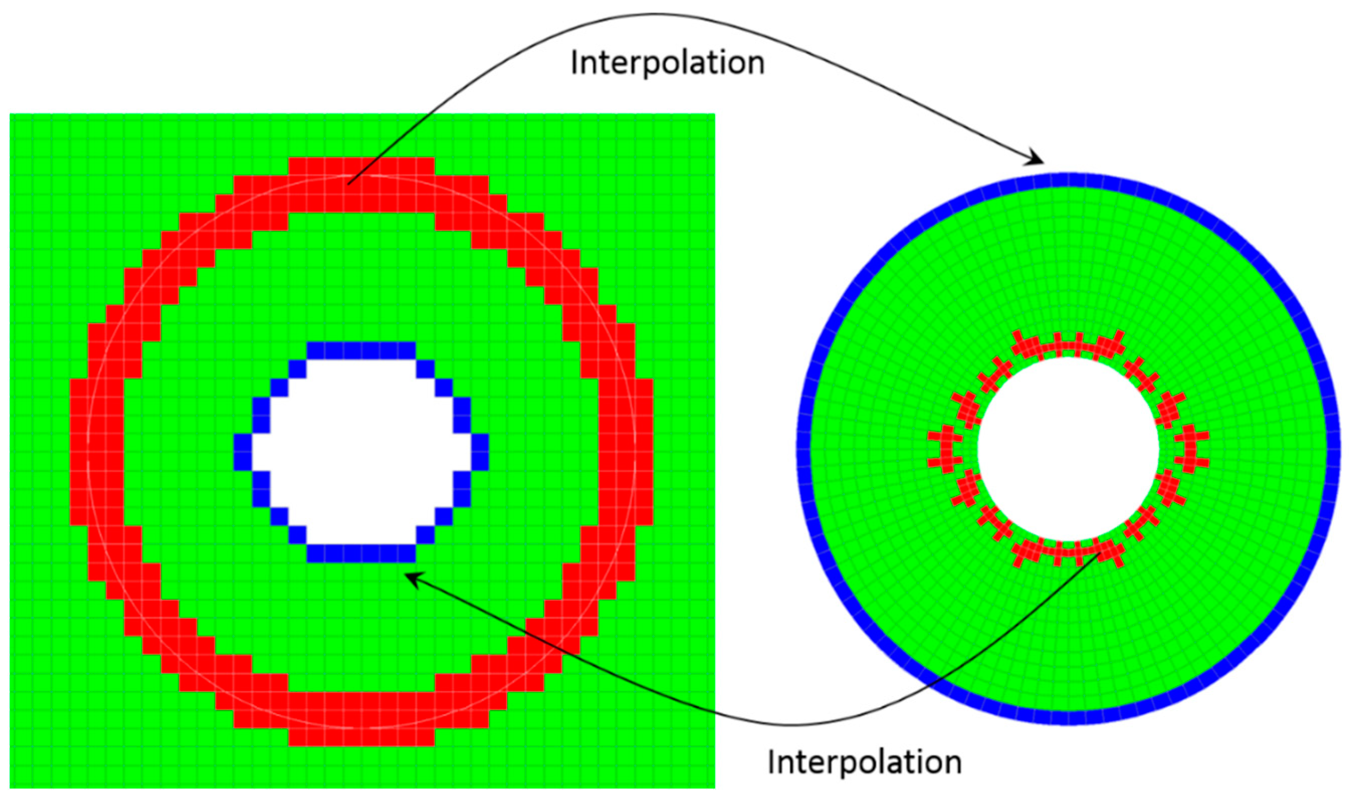
In order to illustrate how the mesh connectivity is established,
Figure 2 shows the overlap of the generic background (left-hand side) and component (right-hand side) grids. On the background grid, the cells encompassed or crossed by wall surfaces of the component grid are deactivated. Then, on the outer boundary of the component grid, the flow quantities are obtained by interpolation from the background grid. In this region, the overlapping grids are created to have approximately the same cell size. The cells receiving solution by interpolation are referred to as “receptor cells” and marked in blue in
Figure 2. The cells selected to provide solution for the receptor cells are addressed as “donor cells” and are marked in red in
Figure 2. Note that the donor cells are a sub-group of the green cells (“solve cells”), where the governing equations are solved. The same mechanism is applied (in reversed direction) to the region around the walls of the component grid to provide boundary conditions to the background grid (blue region in
Figure 2—left). Similar overset techniques have already been applied in aerodynamic models of wind turbines [
26,
27].
2.2. Turbulence Modelling and Modified Wall Functions
The chosen turbulence model is an unsteady RANS, specifically the k-epsilon model, where k represents the turbulent kinetic energy and ε is its dissipation rate. On top of the molecular viscosity, a turbulent viscosity is added and defined as with equal to 0.09 and the density of air (1.225 ).
In order to mimic the ABL stratification under neutral conditions, the inlet conditions proposed by Richard and Hoxey [
28] are adopted for the wind speed,
, and the turbulence quantities, with z the height, thus the distance from the ground wall is:
In these equations, is the ABL friction velocity, representing an index of the global wind intensity, while is the aerodynamic roughness length, providing a measure of the roughness of the ground wall. Lastly, Κ is the von Karman constant (0.4187). These profiles are obtained as analytical solutions of the transport equations of the k-epsilon model.
As observed by Blocken et al. [
29] and Parente et al. [
30], a novel formulation of the ground wall functions is necessary to preserve these inlet profiles throughout the numerical domain. For this reason, the aerodynamic roughness length is accounted for in the wall functions, following the novel formulation proposed and validated by Parente et al. [
31], and obtaining a novel constant, E, and a novel non-dimensional wall distance,
:
where
. This leads to a modified law of the wall for the non-dimensional velocity,
, given by:
In this work, the novel wall functions [
31] presented above are addressed as “modified wall functions” and are adopted on the ground wall (
Figure 1—left), in contrast with the standard ones adopted on the walls of the turbine.
Richard and Hoxey’s ABL profiles are prescribed at the inlet of the domain (
Figure 1), choosing
= 0.671 m/s and
= 0.5 m. At 100 m of height (namely the hub height), this produces a wind velocity of 8.5 m/s. The turbulent kinetic energy is set to 0.0151
. The rotational speed of the rotor is set to 1.445 rad/s, leading to a tip-speed ratio (TSR) of 8.5, thus reproducing the nominal operating conditions as provided by the manufacturer. Given the low Mach numbers obtained in HAWTs, the flow is modelled as incompressible. The continuity and momentum equations are jointly solved in a pressure-based solver. Second order upwind discretization is applied for momentum equations and a first order implicit scheme is used for time discretization. The same settings are used for every simulation presented in this work. The entire setup is implemented in Fluent 18.1 (Ansys Inc., Canonsburg, PA, USA).
2.3. Simulation Scenarios
Several simulations are carried out and compared. First, a “rotor only” (RO) simulation is carried out, placing only the wind turbine rotor in the ABL flow with no misalignment with respect to the incoming wind. Then, the supporting structures are added, leading to the “full machine” (FM) simulation, as previously summarized by
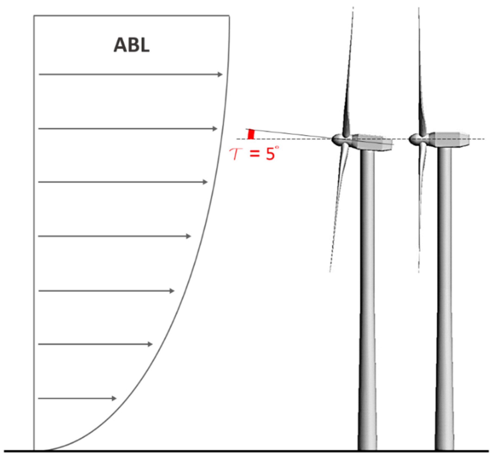
Figure 1—right. The rotor and the nacelle of the machine are subsequently tilted by 5°, as shown in
Figure 3, and as normally done in order to guarantee more blade-tower clearance during the operation of the machine. Lastly, a 5° yaw misalignment is introduced by rotating the whole machine around an axis parallel to its tower, mimicking an incorrect orientation of the turbine. Both the tilt angle and the yaw misalignment are imposed by rotating the rotor around the appropriate axes crossing the center of the rotor, in order to guarantee the same position of this point (and thus exposing the rotor to the same ABL velocity gradient) in every simulation.
Table 1 summarizes the performed simulations, showing the nomenclature to be adopted in the rest of this work and the features associated with each of them.
Each revolution is divided into 240 time steps, so the time step size is 0.0181176 s, and, starting from undisturbed ABL everywhere and wind turbine in stand-still, 6 revolutions are necessary to reach regime in time. Only the seventh revolution is analyzed; the average torque coefficient provided by the turbine during this revolution corresponds to 0.05243 (in the RO configuration), 5.8% off compared to the value provided by the manufacturer (0.0556), and used as a benchmark to validate the employed model.
All the simulations are performed on 10 computational nodes, interconnected by InfiniBand. Each node counts 28 cores of the type Xeon E5-2680v4. With these settings, roughly one day is necessary to perform a complete revolution in any of the presented simulation scenarios, summing up to a week to reach the time regime and obtain meaningful results.
3. Results and Discussion
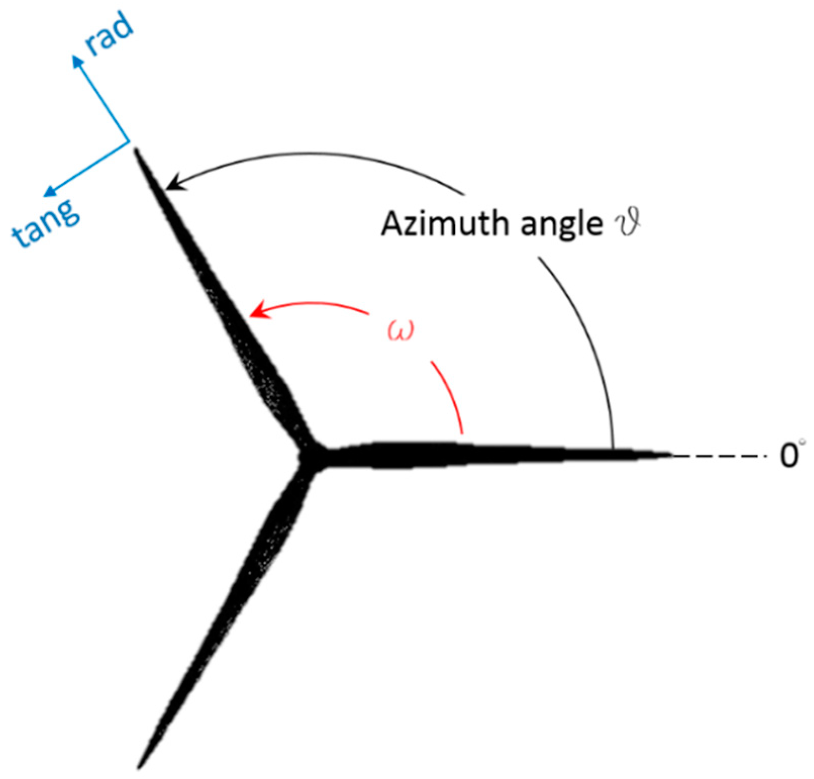
In this section, the results of the performed simulations are analyzed and mutually compared. The notation illustrated in
Figure 4 is used to define the azimuthal position of each blade. A cylindrical coordinate system will be used to define the radial, tangential, and axial (i.e., aligned with the axis of rotation of the machine) directions, according to
Figure 4 and as normally done in the analysis of turbomachines.
Moreover, as usually done in the wind energy field, the torque (T) exerted by the wind flow on the blades is made non-dimensional using the following formula:
where
is the previously defined air density,
the radius of the rotor, and
is the frontal area computed as
. The velocity,
, used in this formula is the undisturbed wind velocity at the hub height, namely 8.5 m/s. In order to allow a more immediate comparison, the frontal area,
, of the untilted and unyawed rotor will always be used when computing the torque coefficient.
In the following sections, analytical calculations of the flow angle on several blade sections will be performed and compared with the obtained CFD results. This is done by reasoning in the cylindrical coordinate system sketched in
Figure 4. The streamwise velocity approaching a generic blade section, whose radial distance from the axis of rotation is
, can be computed from the ABL velocity profile as
, where 100 m corresponds to the hub height,
is the azimuth angle defined in
Figure 4, and τ is the tilt angle (illustrated in
Figure 3 and equal to 0 in the RO and FM configurations). The factor
, is introduced to account for the reduction in the streamwise velocity due to the expansion of the streamtube [
32] and is set to equal 0.75 based on the performed CFD simulations. In the RO and FM configurations, the streamwise velocity coincides with the axial velocity, whereas the tangential and radial wind velocity are equal to 0. In the tilted and yawed configurations, the wind velocity components can be obtained by projecting the streamwise velocity expressed by the previous equation onto the tilted and yawed directions. These directions can be obtained by applying tilt and yaw rotation matrices to the directions valid for the untilted configurations. The axial and tangential wind velocity are then combined with the local blade speed (
, purely tangential) and used to calculate the relative velocity vector,
, impacting on the considered section, by means of the relation,
. Using axial and tangential components of
, the flow angle is calculated.
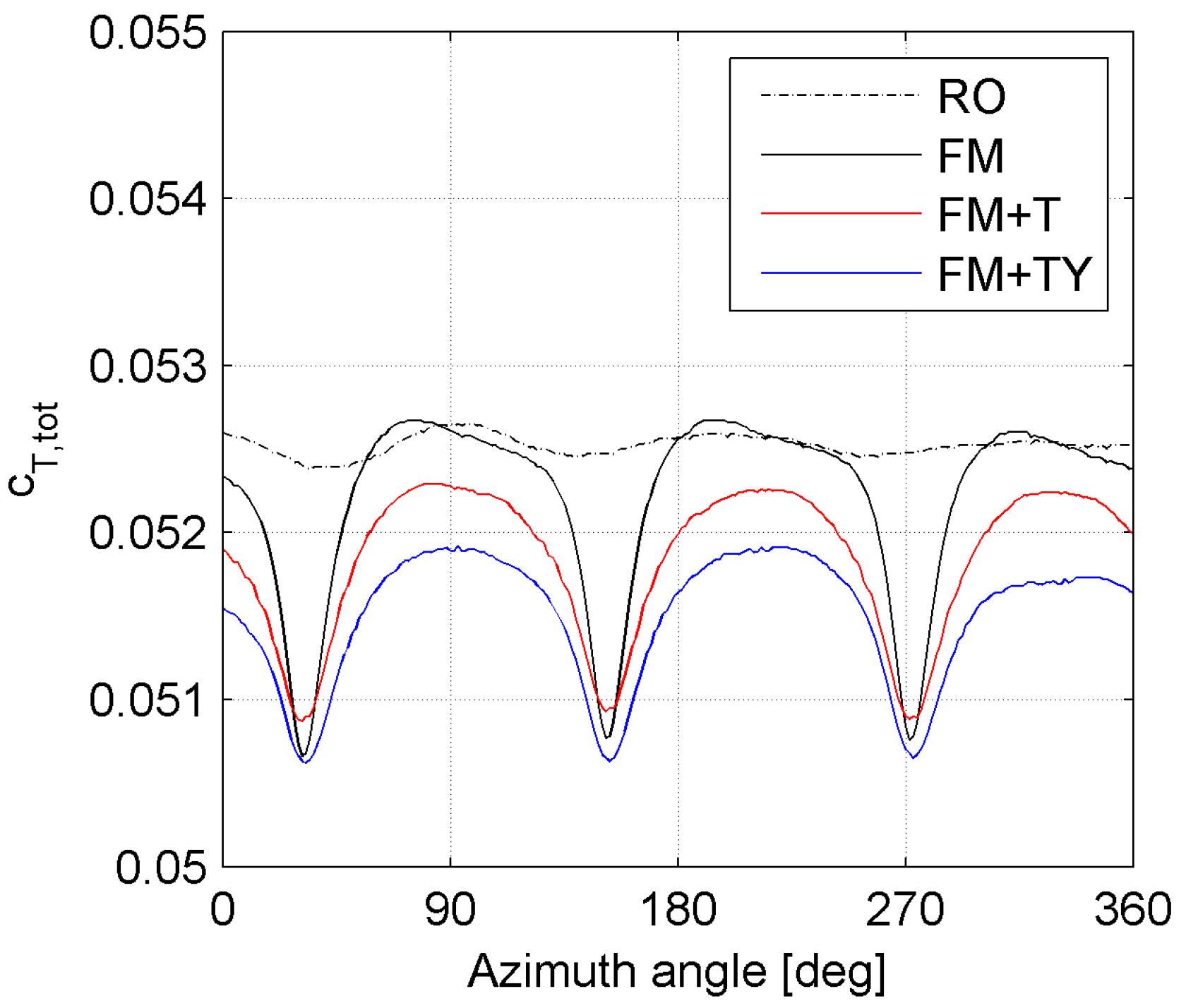
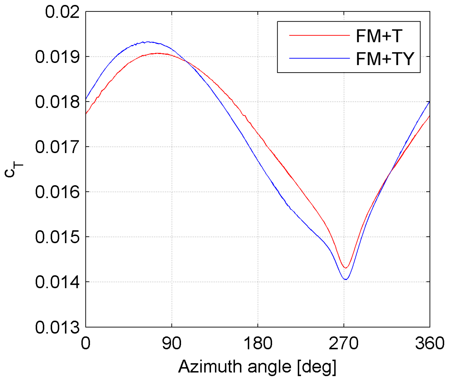
We start with examining the total torque provided by the machine in all the considered configurations (
Figure 5).
In the RO configuration, the total torque coefficient is stable and exhibits only minor oscillations (deviation from average value smaller than 0.3%). Differently, the FM configuration shows a sudden drop (about 3% of the average) in the provided torque every time one of the three blades passes in front of the tower (tower dam effect). This drop is mitigated by the tilt, but the average torque produced is slightly lower (−0.7%). The same effect is further amplified by the yaw misalignment, which reduces the average torque by 0.66% compared to the FM + T configuration. These reductions are to be expected since both the tilt and yaw misalignment have the effect of reducing the rotor frontal area with respect to the incoming wind. However, they are larger than the reduction in the frontal area, which corresponds to only 0.38% for both the tilted and tilted-yawed conditions.
We proceed now with examining a single blade, observing its performance and loading as a function of its azimuth angle. When doing so, the differences in the monitored loads when blades pass the same azimuth angle do not exceed 1%, thus the regime is achieved and the behavior of each blade is representative of the other two.
First, the RO and FM simulations will be compared, in order to identify the influence of the ABL on the dynamics of each blade and show the effect of the presence of the supporting structures. Then, the tilt angle and yaw misalignment are addressed separately in order to clearly display their effects.
3.1. Rotor Only and Full Machine Simulations
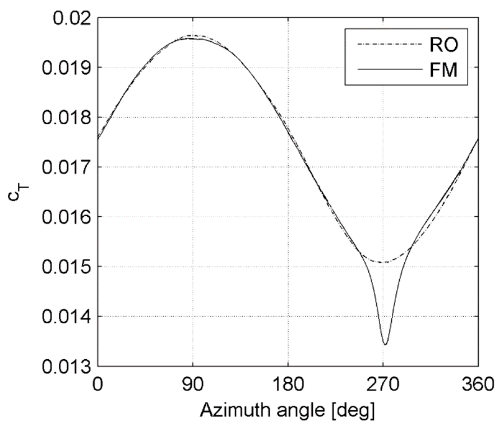
Despite the stability of the total torque, the single blade contribution shows a sinusoidal oscillation in the RO configuration (
Figure 6) as a direct consequence of the ABL.
When the blade points upwards (azimuth angle between 0° and 180°), it is exposed to a higher wind speed and thus the angle of attack over the entire blade is increased, leading to higher torque. The same reasoning reverses when the blade points downwards, i.e., for azimuth angle between 180° and 360°. Qualitatively similar results were obtained in the literature [
13,
14].
The two curves in
Figure 6 almost perfectly overlap, except in the region around 270°, when the blade passes in front of the tower. At this moment, the tower represents an obstruction (tower dam effect) and increases the pressure on the suction side of the blade, reducing its performance. This also translates into a higher peak-to-peak amplitude of the oscillation of the torque.
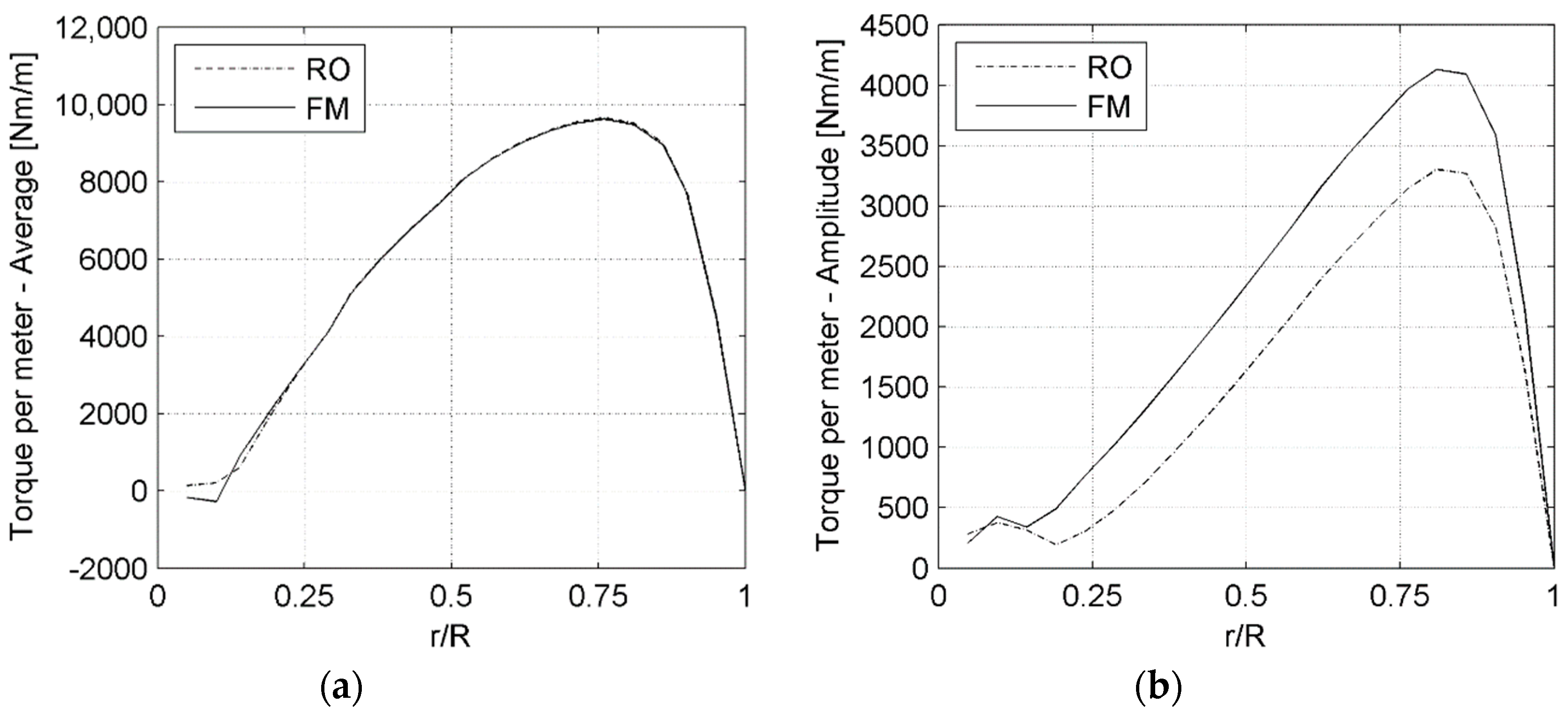
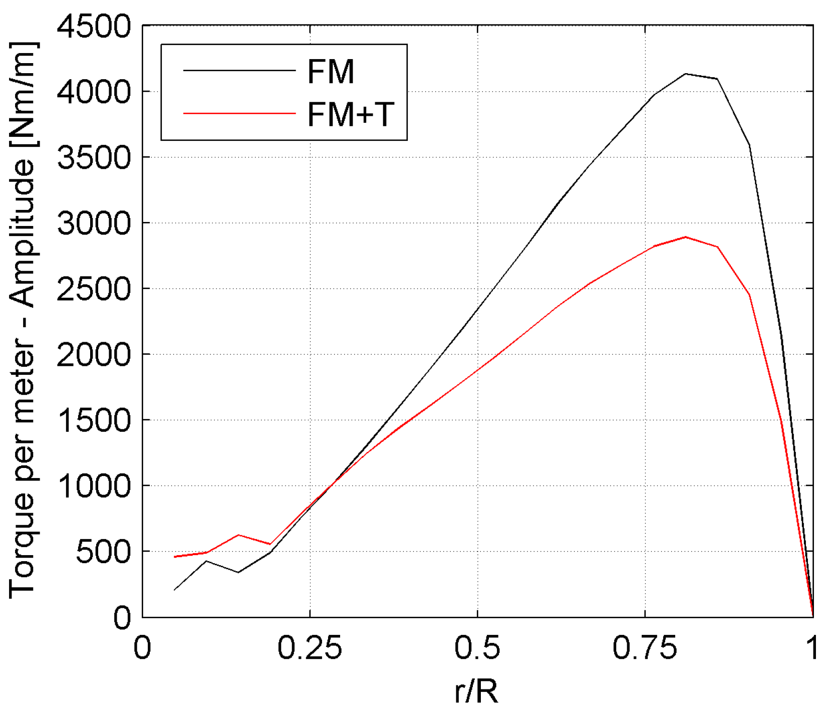
Figure 7 shows the average value (a) and the peak-to-peak amplitude of the oscillation (b) of the torque per meter of blade as a function of the span of the blade, obtained over the full revolution.
Except for the proximity of the root region, the reduction in the average torque value due to the presence of the supporting structures is lower than 0.6%, thus no differences are visible in
Figure 7a. Differently, the peak-to-peak amplitude is consistently increased over the entire blade span (
Figure 7b).
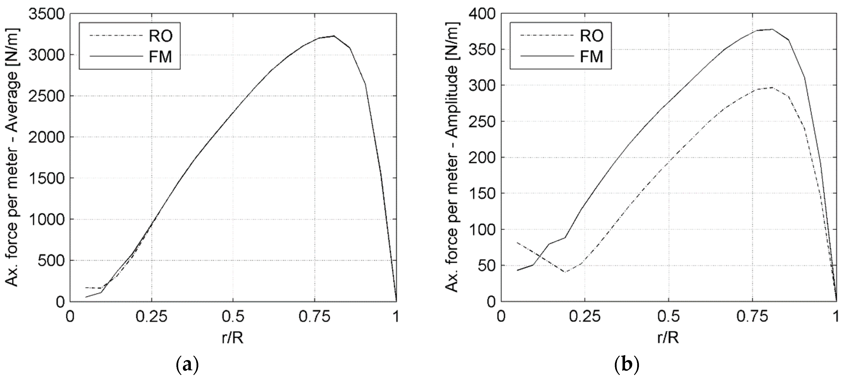
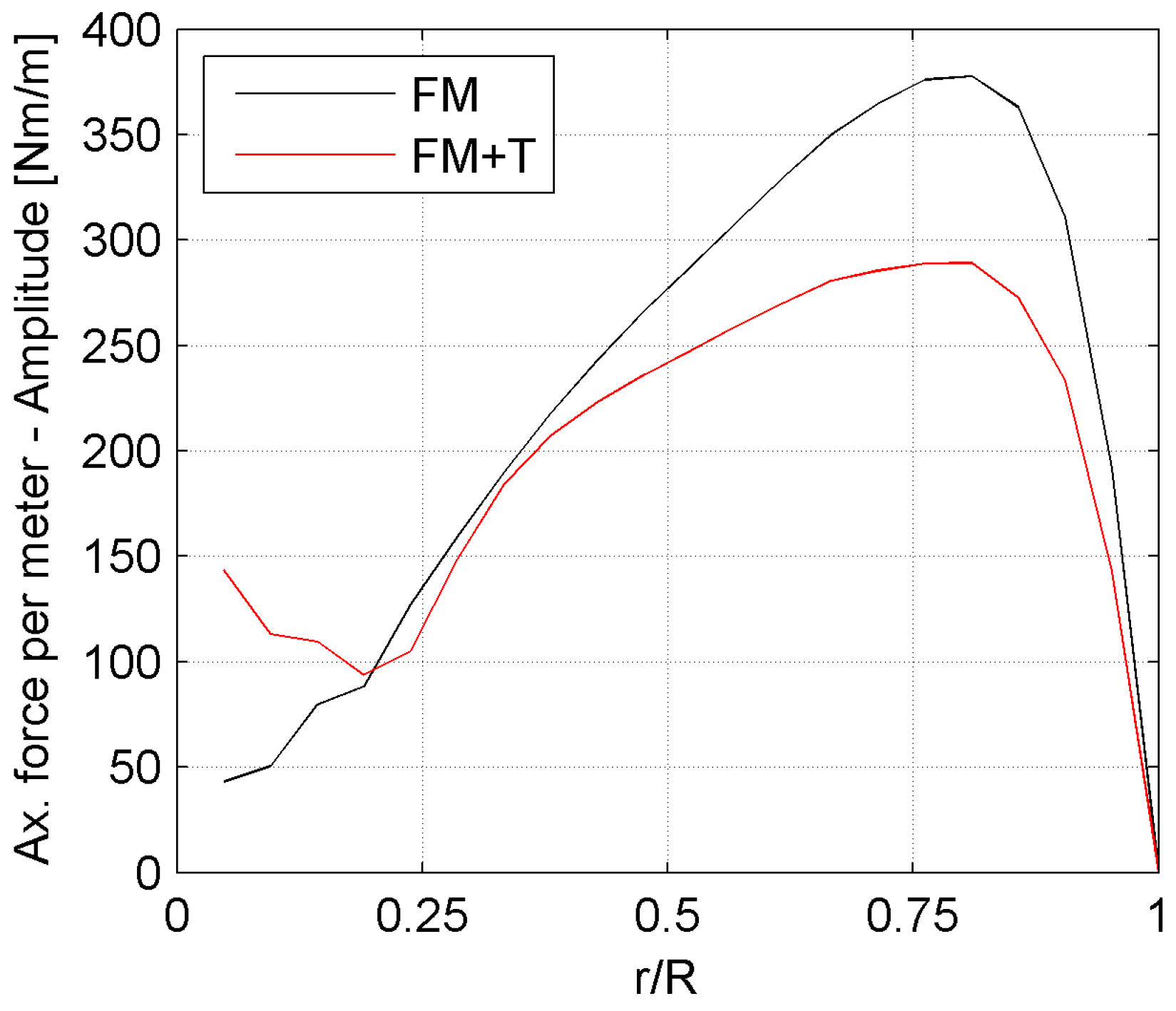
Reasoning similar to that identified for the torque can also be used for the axial force acting on the blade and a similar plot is shown in
Figure 8 for the axial force. This is the most intense sollicitation acting on the blades and also the force responsible for the highest deflections [
27,
33,
34]. Importantly, the consistent increase of its peak-to-peak amplitude of oscillation (
Figure 8a) translates directly into less favorable conditions in terms of the fatigue life of the blade [
35,
36].
3.2. Tilt Angle
Figure 9 shows the torque contribution of the single blade in the FM and FM + T configurations.
The torque in the tilted configuration exhibits both a shift in phase (the positive peak is reached earlier with respect to the untilted configuration) and a decrease in the amplitude of its oscillation. The difference around 270° can be attributed to the higher tower clearance, but the same does not apply to the difference around 90°. The shift in phase and the decrease in amplitude are independent of each other and come, respectively, from the inboard and outboard sections of the blade as shown in
Figure 10. This will now be demonstrated.
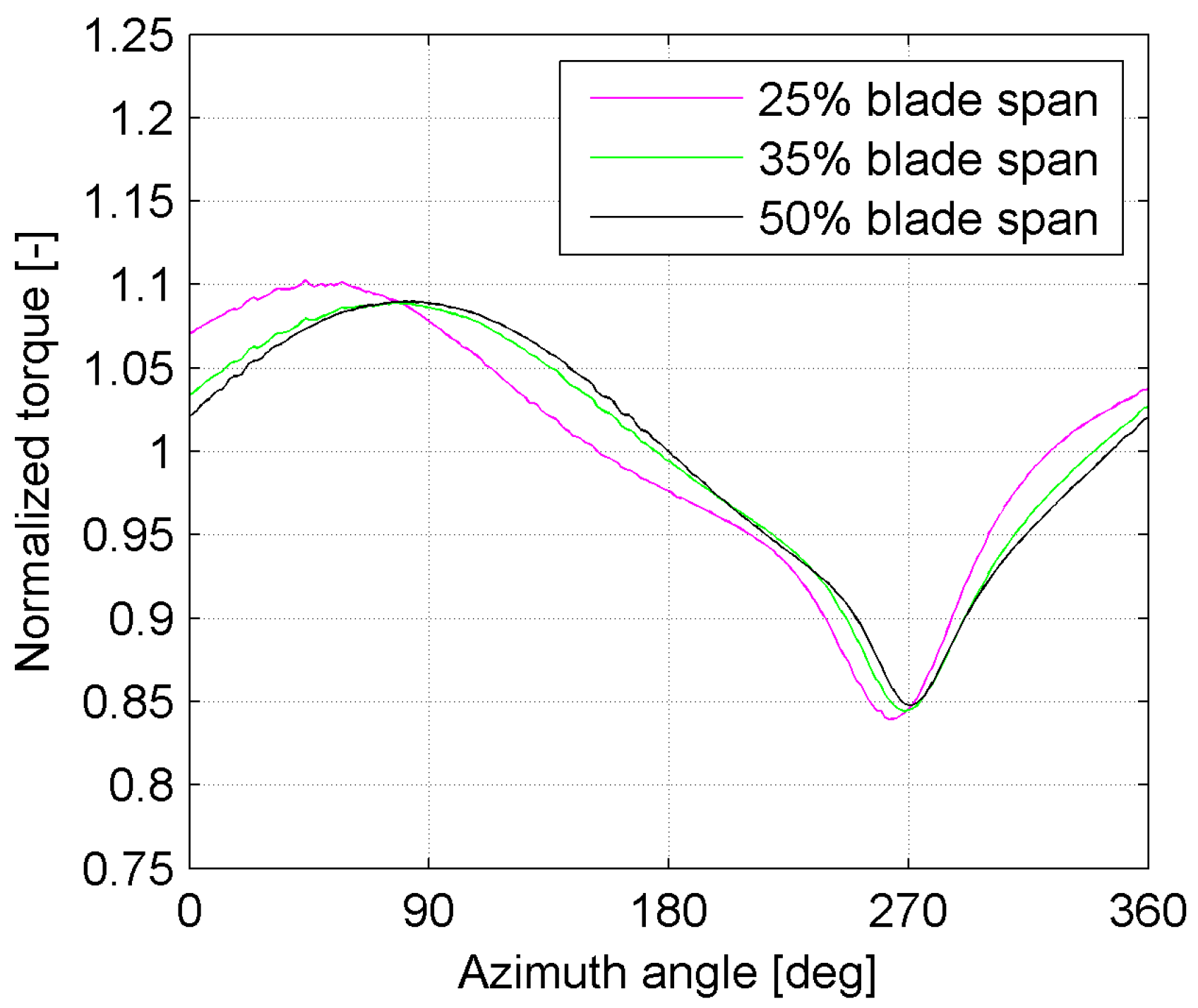
Focusing on the phase shift,
Figure 11 shows the torque provided by different low span sections of the blade, normalized by the respective average value, for the FM + T simulation.
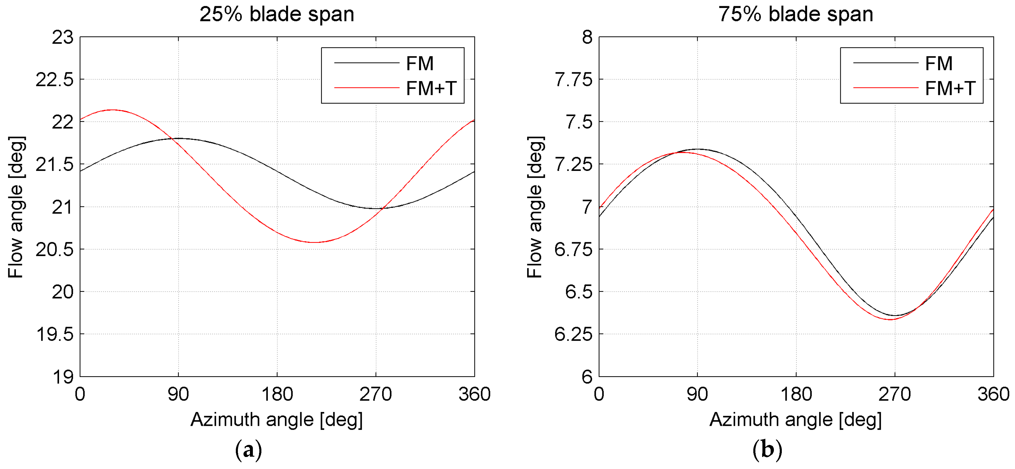
It can be observed that, moving up along the span of the blade, the phase shift gradually disappears and, at 50% of the span, it is no longer observed. This shift can be related to the change in the local angle of attack induced by the tilt angle. Because of this angle, tangential and radial components originate from the wind velocity. The velocity triangles are consequently changed; this translates directly into a different distribution of the angle of attack, which is much more important in the inboard part of the blade, where the blade speed and the wind speed are comparable in magnitude. On the contrary, in the outboard section of the blade, the changes in the wind speed are small compared to the much higher blade speed. The flow angle can be computed as a function of the azimuthal position of the blade at the two examined spanwise locations (
Figure 12).
By comparing
Figure 12 with
Figure 10 and
Figure 11, synchronized peaks (i.e., arising around approximately the same azimuthal position) occurring in the torque and flow angle are observed for the inboard location, while only a minor phase shift is reported in the torque or flow angle at the outboard location. This confirms that the change in the flow angle is the cause for the phase shift close to the hub.
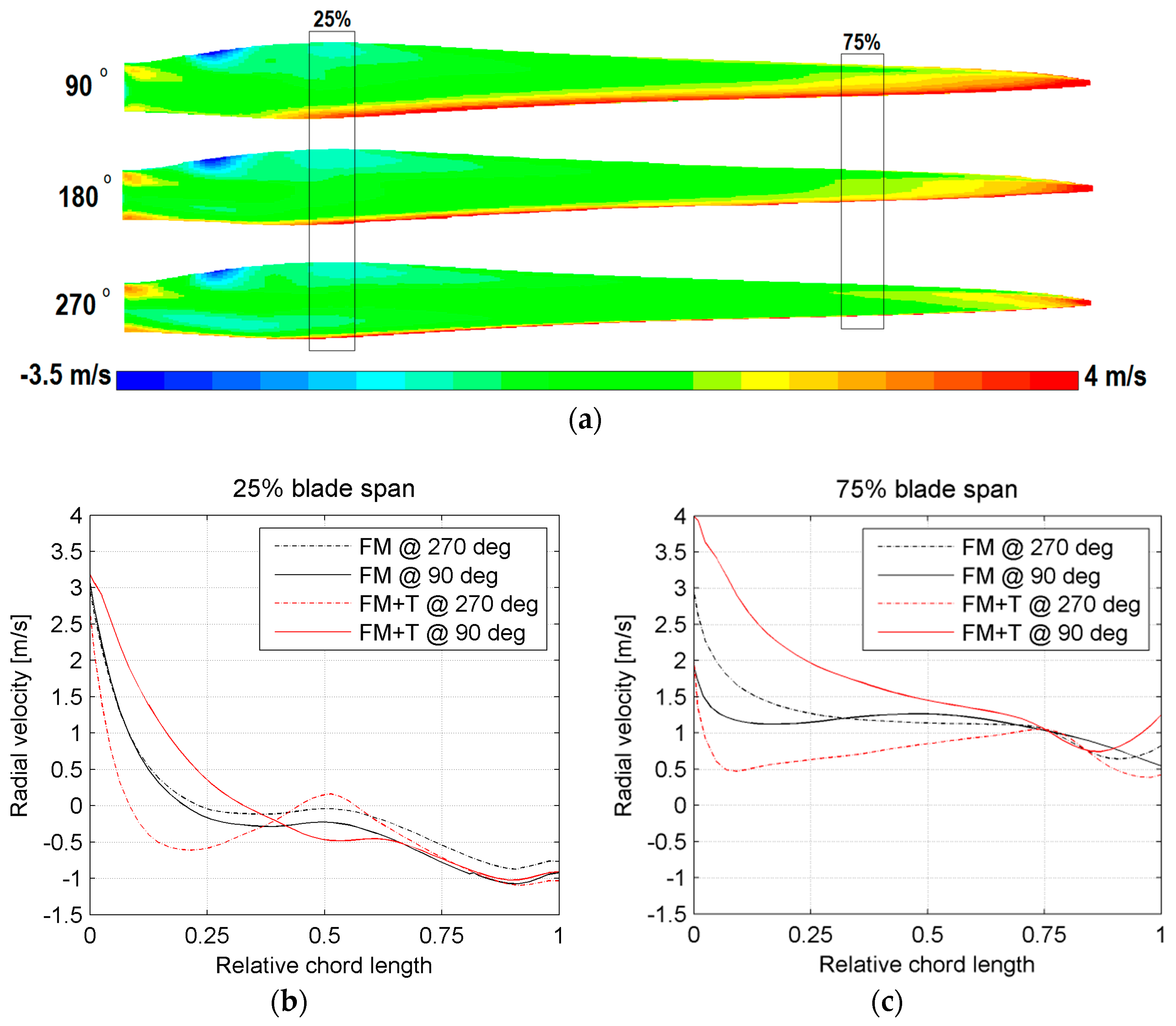
The reduction in amplitude occurring in the torque oscillation of the outboard spanwise location is not observed in the flow angle around the same position. This reduction in torque amplitude is attributed to the radial flow generated by the radial component of the wind velocity impacting on the pressure side of the blades. The radial flow is more intense on the outboard section, since it is directly linked to the recirculation over the blade tip, while it does not sensibly affect the inboard section of the blade (
Figure 13).
A centrifugal flow on the pressure side of the blade will inevitably favor the tip leakage flow (addressed also as “tip loss”) by increasing the amount of fluid circulating over the tip of the blade and towards its suction side, decreasing the efficiency of the energy capture [
8,
9,
32].
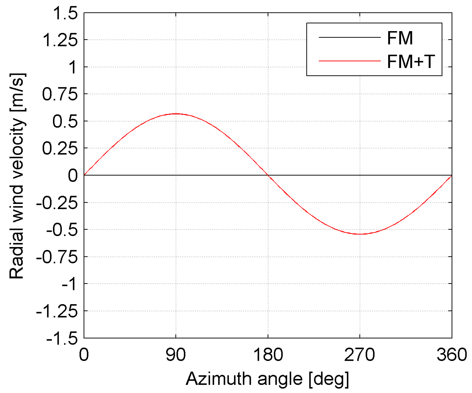
Figure 14 shows the analytically computed radial wind velocity impacting on the location at 75% of the total span.
For an azimuth angle of 270°, the radial velocity (
Figure 13c) in the first cell attached to the blade wall at 75% of the span, averaged over the entire chord length on the pressure side, is 1.23 m/s for the untilted configuration and 0.77 m/s for the tilted configuration. The difference between these numbers (0.46 m/s) is comparable to the analytically computed difference at 270° and equal to 0.54 m/s (
Figure 14). It can be seen that when the impacting radial velocity is positive (i.e., centrifugal), a loss in torque is observed in
Figure 10a. On the contrary, when the impacting radial velocity is negative (i.e., centripetal), a beneficial effect (due to a reduction in the tip loss) is seen, as shown in
Figure 10a.
Figure 15 shows how the reduction in amplitude of the torque oscillation increases towards the tip, where the tip loss has a higher impact on the blade performance [
8,
9,
32] and where the blade distance from the tower gradually increases, due to the imposed tilt angle.
A similar reasoning applies to the axial force; the tilt angle induces a more intense reduction in its oscillation towards the tip, positively impacting on the fatigue life of the blade (
Figure 16). No remarkable change is reported in the distribution of its average value.
3.3. Yaw Angle
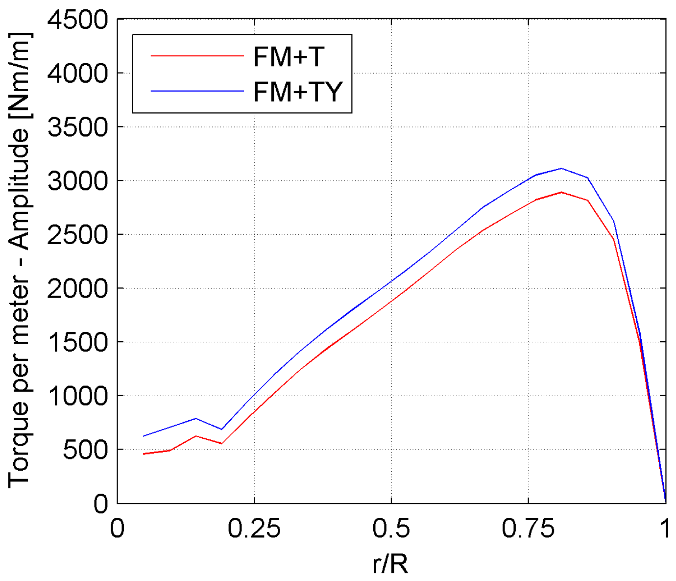
Figure 17 shows the torque contribution of the single blade in the FM + T and FM + TY configurations.
In this case, a further shift in phase (anticipation in the positive peak) is reported, but, contrary to the tilted case, an increase in the amplitude of the oscillation is observed.
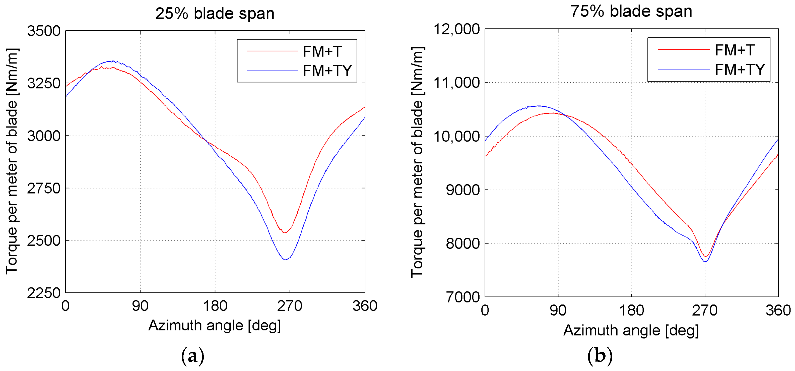
Figure 18 shows the torque contribution at the two previously examined spanwise locations.
A small phase delay is present at the inboard section examined, in contrast with the phase anticipation monitored in the total torque provided by the blade, as well as in the torque contribution of the outboard section. On the other hand, an increase in the amplitude of the torque oscillation is observed on the whole span of the blade (
Figure 19).
The differences in the torque provided by the inboard section can be explained by examining the computed flow angle (
Figure 20a), which exhibits a similar delay in the peak value. Differently, the changes in the torque provided by the outboard section do not find an explanation in the computed flow angle (
Figure 20b).
Figure 20a shows both a delay in the phase and an increase in the amplitude of oscillation, similarly to what is shown for the torque in
Figure 18a. On the other hand, the differences in
Figure 20b are very small compared to the differences in
Figure 18b and the anticipation of the peak observed in the latter is not reported in the flow angle. Similarly to what has been done for the effect of the tilt angle, these differences are related to the different radial flows affecting the outboard part of the blade.
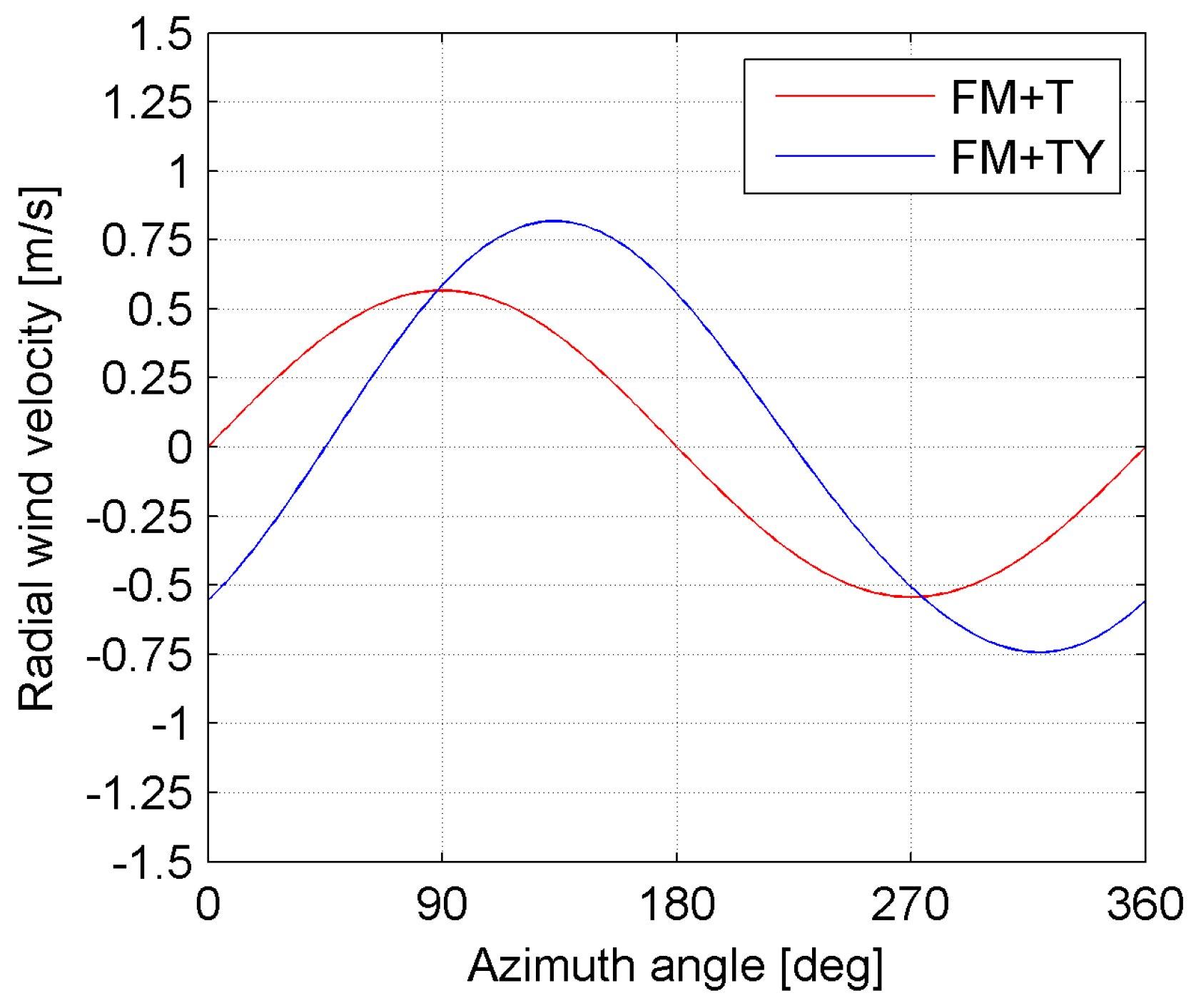
Figure 21 shows the computed radial velocity impacting on the pressure side of the blade in both the tilted and tilted-yawed configuration.
Since a positive velocity denotes a centrifugal flow, which will increase the tip losses and thus reduce the torque production, the difference in radial velocity
is compared to the difference in torque on the outboard location, as shown in
Figure 22.
A global phase agreement is observed, supporting the hypothesized relation between the torque production of the outboard section and the incidence of radial flow and tip losses.
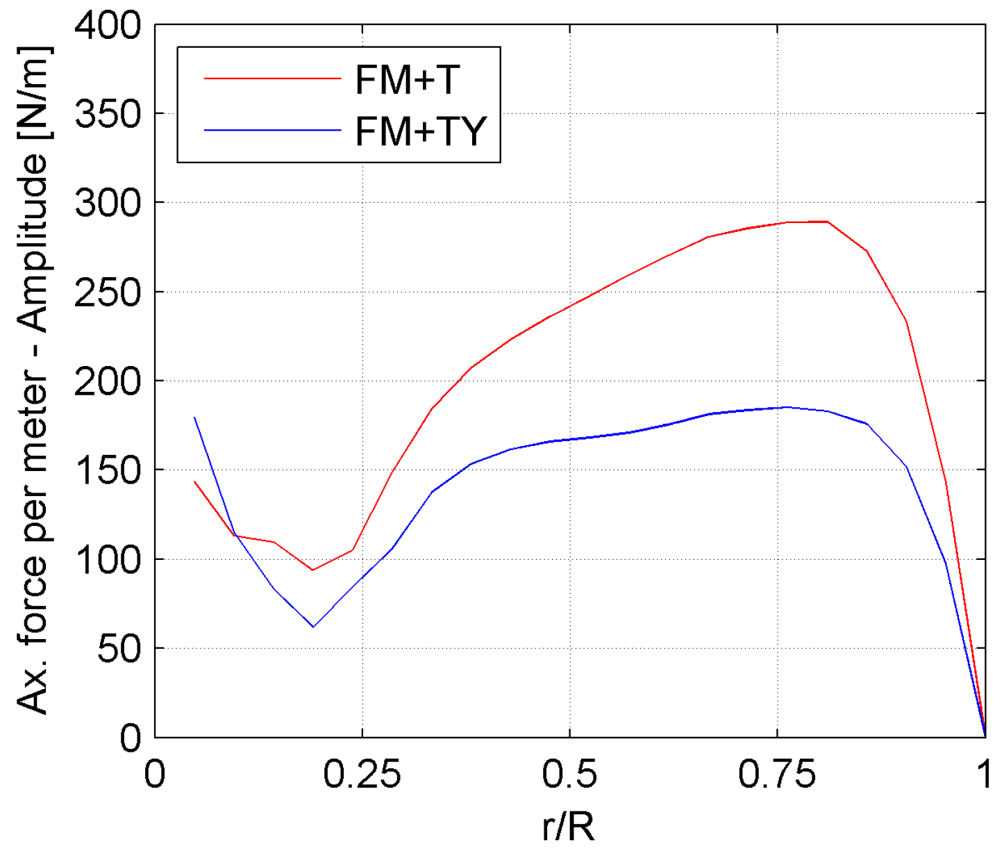
Lastly, the imposed yaw positively influences the amplitude of the oscillation of the axial force acting on the blade, as shown in
Figure 23, leading to more conservative operating conditions in terms of the lifetime of the blades.
4. Conclusions
Several computational fluid dynamics simulations of a 100 m diameter rotor were carried out in order to investigate the effect of the supporting structures and of a rotor tilt and yaw misalignment on the performance and loads of its blades. The machine was immersed in the atmospheric boundary layer in order to account for the wind velocity stratification.
First, the effect of the presence of the supporting structures was analyzed. It leads to a drop in the performance of each blade when it passes in front of the tower. This translates to a fluctuating total torque produced by the turbine and to a bigger amplitude of oscillation of both the torque contribution and the axial force acting on each blade.
Moreover, the effect of tilting the rotor and nacelle of the machine was analyzed. It leads to a less intense fluctuation of both the torque and axial force, leading to a more conservative operating condition for the blades in terms of the fatigue life. On the other hand, it further decreases the average torque produced by the turbine. Different phenomena were observed at the root and the tip of the blade. At the root, the differences in the produced torque are driven by the different distribution of the angle of attack induced by the tilt. On the other hand, these differences are negligible at the tip, where the much higher blade speed makes the velocity triangles insensitive to small changes in the direction of the incoming wind speed. Here, the differences in torque are driven by the different radial flow induced by the tilt, which leads to a difference in tip leakage flow. Similar observations were made for the yawed case, where the amplitude of the oscillating torque provided by each blade was increased.


