Article

Simplified Neural Network Model Design with Sensitivity Analysis and Electricity Consumption Prediction in a Commercial Building

1
Department of Architecture, Xi’an Jiatong-Liverpool University, Suzhou 215123, China
2
Department of Electrical and Electronic Engineering, Xi’an Jiatong-Liverpool University, Suzhou 215123, China
3
Social Science Research Institute, Yonsei University, Seoul 03722, Korea
4
Faculty of Information Technology, Ton Duc Thang University, Ho Chi Minh City 700000, Vietnam
5
Biomedical Engineering Institute, Chiang Mai University, Chiang Mai 50200, Thailand
6
Department of Electrical Engineering, Faculty of Engineering Chiang Mai University, Chiang Mai 50200, Thailand
*
Author to whom correspondence should be addressed.
Energies 2019, 12(7), 1201; https://doi.org/10.3390/en12071201
Submission received: 31 December 2018 / Revised: 15 March 2019 / Accepted: 23 March 2019 / Published: 28 March 2019
(This article belongs to the Special Issue Sustainable Use of Energy in Buildings)

Abstract

:
With growing urbanization, it has become necessary to manage this growth smartly. Specifically, increased electrical energy consumption has become a rapid urbanization trend in China. A building model based on a neural network was proposed to overcome the difficulties of analytical modelling. However, increased amounts of data, repetitive computation, and training time become a limitation of this approach. A simplified model can be used instead of the full order model if the performance is acceptable. In order to select effective data, Mean Impact Value (MIV) has been applied to select meaningful data. To verify this neural network method, we used real electricity consumption data of a shopping mall in China as a case study. In this paper, a Bayesian Regularization Neural Network (BRNN) is utilized to avoid overfitting due to the small amount of data. With the simplified data set, the building model showed reasonable performance. The mean of Root Mean Square Error achieved is around 10% with respect to the actual consumption and the standard deviation is low, which reflects the model’s reliability. We also compare the results with our previous approach using the Levenberg–Marquardt back propagation (LM-BP) method. The main difference is the output reliability of the two methods. LM-BP shows higher error than BRNN due to overfitting. BRNN shows reliable prediction results when the simplified neural network model is applied.

1. Introduction

China’s total electricity consumption in 2015 was 5.55 trillion kWh, and this will increase drastically with China’s economic growth. Specifically, building energy consumption has been emphasized with the increase of urbanization throughout the world. Specifically, in China, it has been projected to drastically increase by 35% by 2020 [1]. Although most buildings are controlled with intelligent energy optimization systems, improving efficiency is still challenging from the power management and microgrid viewpoint. Hence, prediction of building energy consumption has become an important research area, not only regarding energy saving of buildings themselves, but also smart sector organization by way of information communication between buildings. Energy optimization, prediction, and decision-making methodologies have been derived by Carli et al. [2,3,4,5,6,7].
In order to derive a building electricity consumption forecasting model, we use analytical and heuristic modelling. These methods implement a mathematical model and a neural network, respectively. Due to the complex and high dimensional structure, the neural network technique has become one of the main methods to forecast electricity consumption in buildings [5,6,7,8,9,10,11,12,13]. It has also been pointed out that the use of the neural network method has several advantages, such as intelligent processing similar to human thinking, adaptation in various rules, and self-adaptability [14,15]. Supervised learning, back-propagation neural network models show some disadvantages, such as slow convergence, fluctuations, and oscillation during the training process. Furthermore, these models are readily trapped in local minima and it is difficult to determine their network structure [9,15,16,17,18,19]. To remedy these drawbacks, Ye and Kim provided Levenberg–Marquardt back propagation (LM-BP) algorithm to improve the neural network’s low efficiency, slow convergence speed, and limited accuracy [13].
Currently, understanding of the sensitivity of building energy consumption models is important because the sensitivity is closely related with the performance and robustness of the system [20]. In this study, we investigate how different environmental elements, such as temperature, humidity, working day, wind speed, and weather characteristics, influence actual electricity energy consumption in buildings. We propose a novel simplified neural network with the help of mean impact value (MIV) to predict building electricity consumption and to improve the prediction accuracy of building electricity consumption. In order to investigate how each environmental element influences the electricity consumption in a building, we used several neural network algorithms, compared their sensitivity, and suggested a neural network algorithm with a data-driven approach that is well suited to building energy consumption prediction.
We analyzed the sensitivity of neural network building models, because it constitutes a fundamental research background for many building models based on neural networks. The sensitivity analysis yielded important factors that affect building electricity consumption and provides efficient information regarding input variables when there is limited input information.
Sensitivity analyses of neural networks can be categorized into two approaches. The first one is an analytical approach, where the sensitivity is defined as the partial derivative of the output with respect to the input [21,22]. The other is a statistical approach [23]. The analytical approach seems effective; however, there are some limitations, e.g., the fixed weight value and input error have to be zero. The sensitivity is defined as the ratio between the standard deviation of the output error and the input or weight error in the statistical approach. However, there are limitations of both approaches. Both approaches have difficulty in measuring expected output error with respect to overall input patterns [24]. Zeng and Yeung proposed a sensitivity analysis by combining the above two approaches, and derived output variance caused by the perturbation of input and weight. They also pointed out that their result can help to select more weight sets with low sensitivity level during the training [24].
First, sensitivity analysis for the neural network building model is proposed, and the sensitivity is defined in an analytical sense as well. Because the neural network is considered as a black box, we measure the output variation under the perturbation in the input data set, that is, Mean Impact Value (MIV). Naturally, changed output value indicates the influence of input variation on output change, and we can notice that the input data has an important influence on the change of the output variation. This result gives a clue relating to organizing the simplifying the neural network model to avoid unnecessary input. Furthermore, previous results using Levenberg–Marquardt back propagation (LM-BP) for the purpose of electricity prediction has suffered from overfitting due to insufficient data. Hence, we use the Bayesian Regulation Neural Network (BRNN) algorithm to overcome such difficulty. Generally, BRNN provides an appropriate number of neurons to avoid overfitting and underfitting. BRNN is applied to incorporate Bayes’ theorem into the regularization scheme, which is the combination of the conventional sum of the least squares error function with the additional regularization term [25]. The simplified neural network is proposed and verified with the combination of high effective inputs obtained from MIV.
In this paper, we illustrate the sensitivity definition using two Artificial Neural Network algorithms, LM-BP and BRNN, and its relationship with input and output in the next section. In Section 2, sensitivity analysis (SA) is introduced and energy management in buildings and from a residential view point is addressed. Furthermore, SA of the neural network revealed the relationship between energy and neural network structure. More explicit data analysis on neural networks with output variation with respect to input variation has been explained with SA in Section 3. Analysis of the relation between input combination and output is also carried out. Simulation results and the discussion are shown in Section 4. A discussion about the importance of the simplified neural network and the procedure are also addressed Section 4. We also compare the simplified model and original neural network model. Finally, conclusions and future research directions are presented in Section 5.

2. Sensitivity in Neural Network

2.1. Sensitivity Analysis

Sensitivity analysis (SA) analyzes system behavior and characteristics. Hence, SA provides considerable assistance in model building, model identification, and model calibration. Saltelli et al. summarized SA methodologies in their script with quantitative methods and measured the effect of perturbing inputs [26]. Variation of output Y when each conditional input X i satisfies a fixed value x i * is considered a measure of the sensitivity V [ E ( Y | X i = x i * ) ] . It is considered that quantitative approaches, such as variance-based methods or regression methods, are not widely used in engineering or science.
Here, we use a one-at-a-time (OAT) approach, which is also denoted as a direct method. It investigates the change of Y with respect to the variation of X i .
S i = Y X i
It also measures the change of Y due to changes in X i around a nominal value x i * . Equation (1) is expressed as
S i = x i * Y * Y X i
For system analysis (SA), consider the closed loop system in Figure 1. G ( s ) and C ( s ) denote plant and controller or compensator, respectively. r and y represent the reference value and plant output, respectively.
Sensitivity from the reference to output error is represented by the relation S ( s ) : r e = r y . The function can be also expressed as the ratio of change in the closed loop system transfer function to the change of a plant transfer function for a small incremental change [27]. For closed loop, the transfer function satisfies T ( s ) = G ( s ) C ( s ) 1 + G ( s ) C ( s ) ; then, the sensitivity function is defined as S = Δ T ( s ) / T ( s ) Δ G ( s ) / G ( s ) [27].
From a social and environmental viewpoint, SA has been used in energy management for residential areas and buildings [28,29]. Electrical energy purchase and sales price was settled with the help of SA [28]. Another study proposed the use of insulation in external walls, which is the most cost-effective way to save total energy [29].

2.2. Sensitivity Application to Neural Network

2.2.1. Perturbation Relation between Input and Output

Now, we consider a three-layer neural network consisting of one layer for each input, hidden layers, and output layers. The three-layer back propagation (BP) neural network is illustrated in Figure 2. The output of the output layer is expressed as follows [14,16,18,30]:
Y k = f k ( j = 1 l v j k g j ( i = 1 n w i j x i d j ) p k ) ,   j = 1 ,   2 ,   ,   l   and   k = 1 ,   2 ,   ,   m .
In Equation (3), w i j and v j k are the weights between the input and hidden nodes and hidden–output nodes, respectively. n, l, and m are the numbers of input, hidden, and output nodes. d j and p k , j = 1 ,   2 , ,   l , k = 1 ,   2 , ,   m are the threshold of each node. x i , i = 1 ,   2 , ,   n are the input variables for the neural network building model, such as temperature, humidity, working day, and weather characteristics. Y k , k = 1 ,   2 , ,   m are the output variables of the neural network building model, such as electricity consumption, inside room temperature, and so on.
Output variation with respect to input variable, that is Y k x i , is satisfied in for k = 1 ,   2 , ,   m and i = 1 ,   2 ,   ,   n . Derivation of Equation (4) is included in Appendix B.
Y k x i = [ w i 1 w i 2 w i l ] [ v 1 k v 2 k v l k ] .
Therefore, summation of all input perturbation is obtained by P k = i = 1 n Y k x i = j = 1 l i = 1 n w i j v j k for each output, Y k k = 1 ,   2 , , m .
Total perturbation can be accordingly obtained as
E T o T = k = 1 m P k = k = 1 m j = 1 l i = 1 n w i j v j k

2.2.2. Least Square Error

Consider the actual output value F k , k = 1 ,   2 , ,   m , the performance error function in the neural network is expressed from Equation (3) [13,16,17]
E k = 1 2 k ( F k Y k ) 2 = 1 2 k ( F k f k ( j = 1 l v j k g l ( i = 1 n w i j x i d j ) p k ) ) 2 ,   j = 1 ,   2 , ,   l   and   k = 1 ,   2 ,   ,   m
All output error summation is defined as
E L M = i = 1 k E k
In the neural network building model, we define the sensitivity function as error derivation with respect to input variable perturbation. Because the neural network is already trained with the training data, we can assume w i j and v j k are fixed [13]. Sensitivity with respect to input variable is calculated as follows:
k = 1 m E k x i = k = 1 m { ( F k Y k ) f k g j g j x i }
where, f g = j = 1 l v j k , k = 1 ,   2 , ,   m and g j x i = i = 1 n w i j , j = 1 ,   2 ,   ,   l .
Then, it is summarized as
k = 1 m E k x i = ( F k Y k ) k = 1 m j = 1 l i = 1 n v j k w i j
With the comparison between Equations (5) and (9), least square error perturbation analysis is obtained by the multiplication of output error to total perturbation, i.e.,
k = 1 m E k x i = ( F k Y k ) k = 1 m P k

3. Simplified Model Construction

Simplified order modelling is needed to remedy the high dimensional data processing burden. Here, we propose the simplified order model by analyzing the input–output relationship.

3.1. Input–Output Relationship

Actual data of building electricity consumption has been obtained from a shopping mall in Dalian, China. It was also used to validate the model and algorithm in reference [31]. The shopping mall’s area is 50,000 square meters, and it is representative of a high energy consumption building in China. Energy consumption data for March and April in 2014 were included for the analysis. Part of the full data is illustrated in Appendix A.
Neural network output variation is directly affected by the input value variation. It was previously defined as MIV which can be calculated as follows [32]:
  • Train the network with data set M, and get test result and assign as R1.
  • Add a certain proportion, such as p%, into the input data, and make the intended input data set N. Train and get test result as R2.
  • Calculate the difference R1 and R2, which is called MIV.
In our previous result, the results based on MIV were illustrated [13]. In the calculation of MIV, we added p% = 10% variation in input data set M. From Table 1, electricity consumption is highly affected by Temperature and Working Day, i.e., 2.5% and 2.7%, respectively. The negative values of Weather characteristics and Wind speed indicate the opposite direction. So, for each input variable, its absolute value indicates the effect of the variation of the input. From the data illustration in Appendix A, 60 historical data points from the shopping mall were used for training and testing. Forty data points were used for training and 20 data points were used for testing. The wind speed is not considered to affect the input. Every test result, in terms of the RMSE, is greater than the training result.
Based on the environmental condition data, we newly analyzed actual building electricity consumption data and calculated environmental input factors’ influence on sensitivity with MIV information from Table 1. From the calculation, “working day” has the highest influence, followed by “temperature”, “weather”, “humidity”, and “wind speed”. The findings make sense, since working day is rather decisive to electricity consumption, whereas wind speed little effect on electricity consumption because the building is isolated from wind. In order to make simplify, we assign input factors to index. It is illustrated in Table 2.
In order to know how each factor impacts the sensitivity, we also tested the scenarios listed below:
  • {1, 2, 3, 4} = temperature, humidity ratio, working day, weather characteristics
  • {1, 3} = temperature, working day
  • {1, 2} = temperature, humidity
  • {2, 4} = humidity, weather characteristics
  • {3, 4} =working day, weather characteristics
  • {1, 2, 3} = temperature, humidity ratio, working day
  • {1, 2, 4} = temperature, humidity ratio, weather characteristics
  • {1, 3, 4} = temperature, working day, weather characteristics
The Levenberg–Marquardt back propagation (LM-BP) algorithm shows good performance in training, with full input variables presented in Table 3. Regarding the error between the actual electrical consumption and the predicted value, the RMSE value is 223.6 and has low standard deviation. The other simplified input combination results also achieve satisfactory training results with low RMSE. However, the test results do not show consistency. The prediction error variation is very large. This is due to the insufficiency of the small amount of data. Thus, LM-BP is not a reliable neural network prediction model. Hence, we consider different neural network models to replace LM-BP. With the consideration of Equations (4) and (5), it is very clear that the input–output relationship is affected by weight values, w i j and v j k . It is proper to include weight information in the cost function. Thus, we apply a Bayesian regularization neural network to construct a neural network model more suitable for small amounts of data.

3.2. Bayesian Regularized Neural Network

Bayesian Regularized Neural Network (BRNN) also constitutes a multilayer structure for the nonlinear regression. It has hidden layers and weight connections between nodes like Figure 2. BRNN is assessed with the error of least square as in Equation (7) and the regularization term, E w . It penalizes large values of node connection weight. For total output error summation, E L M = i = 1 k E k is defined as above in Equation (7). Error with regularization consideration is defined in Equation (11) [33,34].
E = β E L M + α E w
where, E w = i = 1 m w i 2 , w i and m denote weight and number of weights, respectively. With the help of Bayesian network theory, regularization parameters α and β are obtained [25,34].
With the regularization objective function in Equation (11), extensive work on Bayes’ rule to neural network training and regularization was done by MacKay [34]. The weight density function can be updated from the Bayes’ rule as follows [25]:
P ( w | D ,   α ,   β ,   M ) = P ( D | w ,   β ,   M ) P ( w | α ,   M ) P ( D | α ,   β ,   M )
where D , M , and w denote the data set, particular neural network model, and network weight vector, respectively [34]. As Bishop proposed, with initial prior distribution and data observation, it is converted to a posterior distribution with the help of Bayes’ theorem [35]. Posterior density P ( w | D ,   α ,   β ,   M ) is obtained via Gaussian prior density and a likelihood function. The regularization parameters α and β are also obtained through Hessian availability [25].

4. Discussion

In Table 3, input variables are indexed; then, ten combinations of input variables are considered by excluding null inputs, single inputs, and whole inputs. In Table 4, training and test results from BRNN with ten reduced input combinations are illustrated. Training and test results with full input variables have RSME means of 571.6877 and 1168.5, respectively. The results show higher RMSE values than the LM-BP test results [13]. However, 100 iterations of the testing shows rather reliable standard deviation, 1.3711 × 10⁻¹².
Among all input combinations, the most expected {Temperature, Working Day} = {1, 3} input combination shows reliable output compared with full input case. By inspection, the rather high RMSE results come from the combinations of {1, 2}, {2, 4}, and {1, 2, 4}. We can see that the common input in these combinations is “Humidity”. Hence, we will investigate why {Humidity} = {2} is not related to electricity consumption.
Now, simulation is planned for
  • Simulate full input {1, 2, 3, 4} and two inputs {1, 2}. Compare with actual test data.
  • Simulate full input {1, 2, 3, 4} and two inputs {1, 3}. Compare with actual test data.
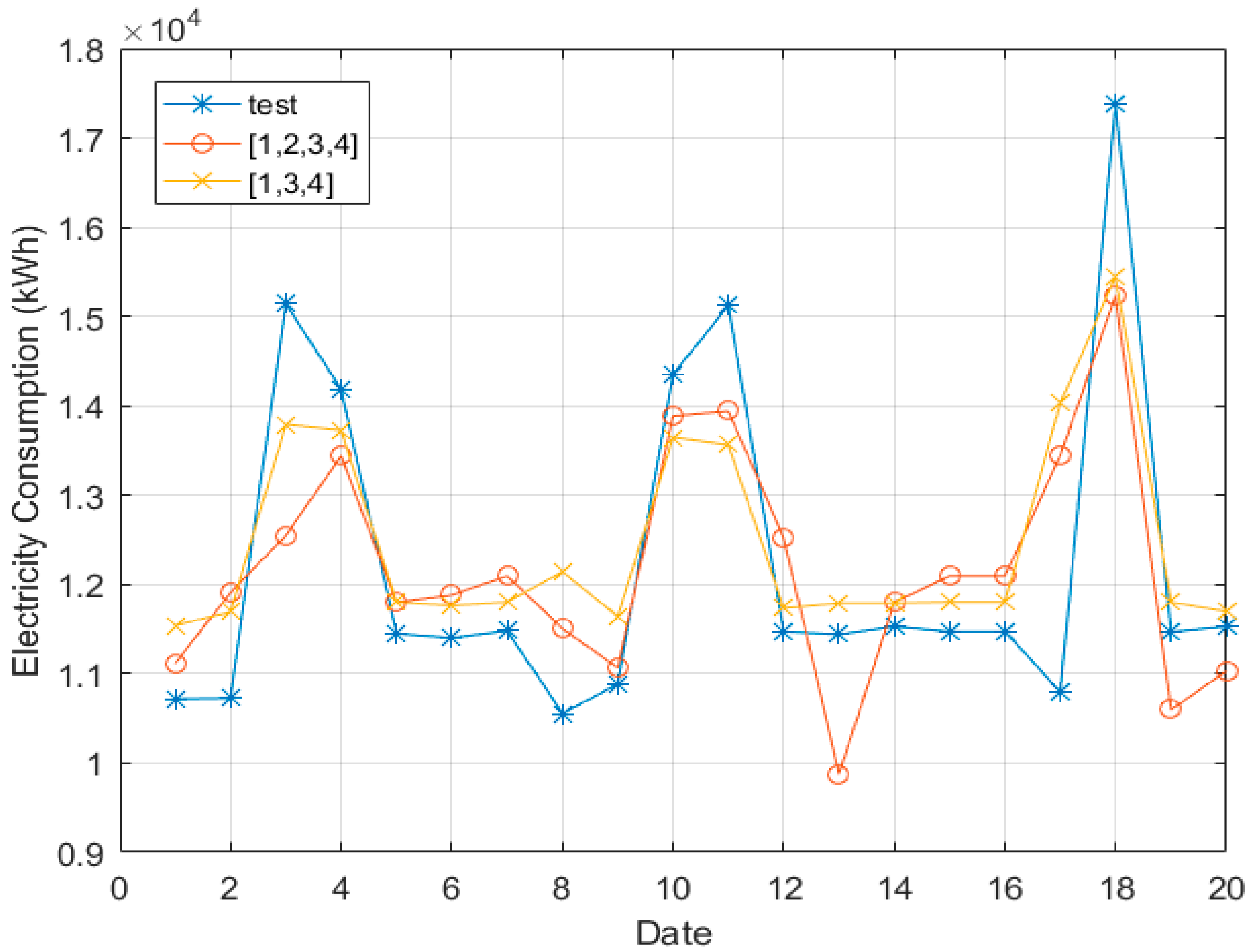
  • Simulate full input {1, 2, 3, 4} and three inputs {1, 3, 4}. Compare with actual test data.
From the simulation results, we investigate how “Humidity” and two inputs {Temperature, Working Day} affect building electricity consumption. As illustrated in Figure 3, input {1, 2} with humidity results does not guarantee agreement with the test value. This means that “Humidity” is not a predictor of energy consumption. From Figure 3, the results are consistent due to low standard deviation, but the prediction results do not follow actual test data.
From Figure 4 and Figure 5, the predictions with input combinations of {1, 3} and {1, 3, 4} are similar. The output results also show consistency, with very low standard deviations for both. From the simulation results, it is obvious that the {Temperature, Working Day} = {1, 3} input combination is a good predictor of electricity consumption. It is also pointed out that the simulation results with BRNN are more satisfactory than with LM-BP in terms of reliability [8].
In the previous results reported in the literature, the absolute relative errors of the predicted output values were between 0.314% and 11.635% with the LM-BP neural network [13]. Although the resulting error rate was lower than for the BP neural network, it has a high standard deviation. This means that the method is not reliable, while for BRNN, every case of our test result in Table 4 shows a rather small standard deviation. As mentioned, LM-BP cannot guarantee high reliability with a small amount of data due to overfitting.
The simplified NN model provides easy, fast, efficient, and reliable results. From the fixed system point of view, overall system order must be reduced by way of controller design. The neural network model is organized by way of a training procedure, and the model is optimized by the specific combination of the data set. Thus, weight smoothness is needed to satisfy the balanced and regularized requirements. Although it has a long historical background, Bayesian knowledge cannot obtain the output density function from the likelihood function and prior density.
P ( y k | α ,   β ) = P ( α ,   β | y k ) P ( y k ) t o t a l   p r o b a b i l i t y .
It provides a simpler solution [18,19], but still needs the likelihood function in advance.

5. Conclusions

In this study, we proposed a simplified neural network with the help of mean impact value (MIV) to predict building electricity consumption. In order to investigate how each environmental element influences the electricity consumption in a building, we analyzed the sensitivity using the Bayesian neural network. A Bayesian regularization neural network (BRNN) was applied to a shopping mall building model to describe the input–output relationship. In order to design a simplified NN, SA was addressed. The definition of SA and its application in feedback systems and residential/building case studies were explained. The relationship between total energy and input variables in NN were derived. As we pointed out, the simplified neural network model makes it possible to avoid repetitive calculation and provides a faster response than a full-scale neural network structure. First, we applied MIV to the BRNN model to add and subtract 10% as described in Section 3.1. Wind speed has very low MIV, hence it was excluded from model input. Ten selected input combinations were applied to the simplified model, and the prediction results were obtained. The results were rather reliable; we simulated the prediction 100 times and they yielded rather low standard deviation of the error. From the simulation results, it was verified that the humidity variable is the least influential on energy consumption in the building model. It is clear from the simulation results that temperature and working day are the strongest predictors of energy consumption. In the future, we could analyze the electricity consumption impact and sensitivity of other environmental elements, such as seasonal climate change, occupancy behavior, lighting types, and mechanical systems.
The obtained results are helpful for designing simplified neural networks. Our light model can be extended to residential houses and small microgrids as well. From the simulation results, we also verified that the BRNN model is suitable for describing neural networks with small amounts of data. Using the simplified model, a smart device can be installed to control the energy consumption of buildings.

Author Contributions

Conceptualization, M.K.K.; methodology, J.C. and S.L.; software, V.H.P.; validation, S.L. and N.T.-U.; resources, M.K.K.; writing—review and editing, S.L.; supervision, M.K.K. and N.T.-U.; funding acquisition, S.L. In final proof, E.L. helped to complete SA on energy management, specifically in residential view point.

Funding

This research was funded by RDF from XJTLU, grant number RDF 14-03-11.

Acknowledgments

Authors appreciate to the support CeSGIC from XJTLU to finish the research article.

Conflicts of Interest

All authors confirmed that there is no conflict of interest.

Appendix A

Historical electricity consumption data of a shopping mall in Dilian, China. Data is from 1st of March to 29th of April. The input data are Temperature (°C), Humidity (%), Working Day—working (1) and holiday (0), and Weather condition—cloudy, sunny, and other conditions are classified.
Table A1. Shopping mall historical data [28].
DateTemperature (°C)Humidity (%)Working DayWeather CharacteristicsElectricity Consumption (kWh)
03.0154200.813958
03.026310113529
03.0364610.89148
03.0447810.612071
03.05346117711
03.06533118734
03.07429118748
04.2420301111473
04.2520301111473
04.26165700.710795
04.27156800.517385
04.2820391111470
04.29214610.811531

Appendix B

Output variation obtained based on input change can be expressed as follows:
Y 1 x 1 = i = 1 l v i 1 w 1 i = v 11 w 11 + v 21 w 12 + + v l 1 w 1 l Y 1 x 2 = i = 1 l v i 1 w 2 i = v 11 w 21 + v 21 w 22 + + v l 1 w 2 l Y 1 x n = i = 1 l v i 1 w n i = v 11 w n 1 + v 21 w n 2 + + v l 1 w n l Y 2 x 1 = i = 1 l v i 2 w 1 i = v 12 w 11 + v 22 w 12 + + v l 2 w 1 l Y 2 x 2 = i = 1 l v i 2 w 2 i = v 12 w 21 + v 22 w 22 + + v l 2 w 2 l Y 2 x n = i = 1 l v i 2 w n i = v 12 w n 1 + v 22 w n 2 + + v l 2 w n l Y m x 1 = i = 1 l v i m w 1 i = v 1 m w 11 + v 2 m w 12 + + v l m w 1 l Y m x 2 = i = 1 l v i m w 2 i = v 1 m w 21 + v 2 m w 22 + + v l m w 2 l Y m x n = i = 1 l v i m w n i = v 1 m w n 1 + v 2 m w n 2 + + v l m w n l
The results are summarized as the following matrix; the first output perturbation has the following expression:
[ Y 1 x 1 Y 1 x 2 Y 1 x n ] = [ w 11 w 12 w 21 w 22 w 1 l w 2 l w n 1 w n 2 w n l ] [ v 11 v 21 v l 1 ]
Successive output variations are illustrated in the following equation:
[ Y 2 x 1 Y 2 x 2 Y 2 x n ] = [ w 11 w 12 w 21 w 22 w 1 l w 2 l w n 1 w n 2 w n l ] [ v 12 v 22 v l 2 ]   and   [ Y m x 1 Y m x 2 Y m x n ] = [ w 11 w 12 w 21 w 22 w 1 l w 2 l w n 1 w n 2 w n l ] [ v 1 m v 2 m v l m ]
Then, each output perturbation with respect to inputs is obtained as in Equation (4).

References

  1. Administration, N.E. National Energy Administration in China. 2015. Available online: http://www.nea.gov.cn/2016-01/15/c_135013789.htm (accessed on 1 December 2018).
  2. Xie, Q.; Ouyang, H.; Gao, X. Estimation of electricity demand in the residential buildings of China based on household survey data. Int. J. Hydrog. Energy 2016, 41, 15879–15886. [Google Scholar] [CrossRef]
  3. Carli, R.; Dotoli, M.; Pellegrino, R.; Ranieri, L. A decision making technique to optimize a building stock energy efficiency. IEEE Trans. Syst. Man Cybern. Syst. 2017, 47, 794–807. [Google Scholar] [CrossRef]
  4. Pacheco-Torres, R.; Heo, Y.; Choudhary, R. Efficient energy modelling of heterogeneous building portfolios. Sustain. Cities Soc. 2016, 27, 49–64. [Google Scholar] [CrossRef] [Green Version]
  5. Carli, R.; Dotoli, M.; Pellegrino, R. A Hierarchical Decision Making Strategy for the Energy Management of Smart Cities. IEEE Trans. Autom. Sci. Eng. 2017, 14, 505–523. [Google Scholar] [CrossRef]
  6. Dall’O’, G.; Norese, M.F.; Galante, A.; Novello, C. A Multi-Criteria Methodology to Support Public Administration Decision Making Concerning Sustainable Energy Action Plans. Energies 2013, 6, 4308–4330. [Google Scholar] [CrossRef] [Green Version]
  7. Carli, R.; Dotoli, M. Energy scheduling of a smart home under nonlinear pricing. In Proceedings of the 2014 IEEE 53rd Conference on Decision and Control (CDC), Los Angeles, CA, USA, 15–17 December 2014; pp. 5648–5653. [Google Scholar]
  8. Ahmad, M.W.; Mourshed, M.; Rezgui, Y. Trees vs. Neurons: Comparison between random forest and ANN for high-resolution prediction of building energy consumption. Energy Build. 2017, 147 (Suppl. C), 77–89. [Google Scholar] [CrossRef]
  9. Ahmad, M.W.; Mourshed, M.; Yuce, B.; Rezgui, Y. Computational intelligence techniques for HVAC systems: A review. Build. Simul. 2016, 9, 359–398. [Google Scholar] [CrossRef] [Green Version]
  10. Hsu, D. Comparison of integrated clustering methods for accurate and stable prediction of building energy consumption data. Appl. Energy 2015, 160 (Suppl. C), 153–163. [Google Scholar] [CrossRef] [Green Version]
  11. Shi, G.; Liu, D.; Wei, Q. Energy consumption prediction of office buildings based on echo state networks. Neurocomputing 2016, 216 (Suppl. C), 478–488. [Google Scholar] [CrossRef]
  12. Tetlow, R.M.; van Dronkelaar, C.; Beaman, C.P.; Elmualim, A.A.; Couling, K. Identifying behavioural predictors of small power electricity consumption in office buildings. Build. Environ. 2015, 92 (Suppl. C), 75–85. [Google Scholar] [CrossRef]
  13. Ye, Z.; Kim, M.K. Predicting electricity consumption in a building using an optimized backpropagation and Levenberg-Marquardt back-propagation neural network: Case study of a shopping mall in China. Sustain. Cities Soc. 2018, 42, 176–183. [Google Scholar] [CrossRef]
  14. Neto, A.H.; Fiorelli, F.A.S. Comparison between detailed model simulation and artificial neural network for forecasting building energy consumption. Energy Build. 2008, 40, 2169–2176. [Google Scholar] [CrossRef]
  15. Werbos, P. Beyond Regression: New Tools for Prediction and Analysis in the Behavioral Sciences. Ph.D. Thesis, Harvard University, Cambridge, MA, USA, 1975. [Google Scholar]
  16. Azadeh, A.; Ghaderi, S.F.; Sohrabkhani, S. Annual electricity consumption forecasting by neural network in high energy consuming industrial sectors. Energy Convers. Manag. 2008, 49, 2272–2278. [Google Scholar] [CrossRef]
  17. Zhong, B.; Lu, K.; Lv, D.; Luo, J.; Fang, X. Short-term Prediction of Building Energy Consumption Based on GALM Neural Network. In Proceedings of the International Conference on Advances in Mechanical Engineering and Industrial Informatics, Zhengzhou, China, 11–12 April 2015. [Google Scholar]
  18. Ekici, B.B.; Aksoy, U.T. Prediction of building energy consumption by using artificial neural networks. Adv. Eng. Softw. 2009, 40, 356–362. [Google Scholar] [CrossRef]
  19. Kumar, R.; Aggarwal, R.K.; Sharma, J.D. Energy analysis of a building using artificial neural network: A review. Energy Build. 2013, 65, 352–358. [Google Scholar] [CrossRef]
  20. Doyle, J.C.; Francis, B.A.; Tannembaum, A.R. Feedback Control Theory; Macmillan Publishing Company: London, UK, 1992. [Google Scholar]
  21. Hashem, S. Sensitivity analysis for feedforward artificial neural networks with differentiable activation functions. In Proceedings of the IJCNN 92, Baltimore, MD, USA, 7–11 June 1992; Volume 1, pp. 419–424. [Google Scholar]
  22. Fu, L.; Chen, R. Sensitivity analysis for input vector in multilayer feedforward neural network. In Proceedings of the IEEE International Conference Neural Networks, San Francisco, CA, USA, 28 March–1 April 1993; Volume 1, pp. 215–218. [Google Scholar]
  23. Choi, J.Y.; Choi, C.H. Sensitivity analysis of multilayer perceptron with differentiable activation functions. IEEE Trans. Neural Netw. 1992, 3, 101–107. [Google Scholar] [CrossRef] [PubMed]
  24. Zeng, X.; Yeung, D.S. Sensitivity analysis of multilayer perceptron to input and weight perturbations. IEEE Trans. Neural Netw. 2001, 12, 1358–1366. [Google Scholar] [CrossRef] [PubMed]
  25. Foresee, F.D.; Hagan, M.T. Gauss-Newton approximation to Bayesian learning. In Proceedings of the 1997 International Joint Conference on Neural Networks, Houston, TX, USA, 12 June 1997; pp. 1930–1935. [Google Scholar]
  26. Saltelli, A.; Tarantola, S.; Campolongo, F. Sensitivity analysis as an ingredient of modelling. Stat. Sci. 2000, 15, 377–395. [Google Scholar]
  27. Dorato, P. (Ed.) Robust Control; IEEE Press: Piscataway, NJ, USA, 1987. [Google Scholar]
  28. Cucchiella, F.; D’Adamo, I.; Gastaldi, M. Economic Analysis of a Photovoltaic Systems: A Resource for Residential Households. Energies 2017, 10, 814. [Google Scholar] [CrossRef]
  29. Biserni, C.; Valdiserri, P.; D’Orazio, D.; Garai, M. Energy Retrofitting Strategies and Economic Assessment: The Case Study of Residential Complex Using Utility Bills. Energies 2018, 11, 2055. [Google Scholar] [CrossRef]
  30. Wong, S.L.; Wan, K.K.W.; Lam, T.N.T. Artificial neural networks for energy analysis of office buildings with daylighting. Appl. Energy 2010, 87, 551–557. [Google Scholar] [CrossRef]
  31. Liu, Z.P. Research and Design of Wireless Monitoring System for Building Energy Consumption. Master’s Thesis, Dalian University of Technology, Dalian, China, 2015. (In Chinese). [Google Scholar]
  32. Zhang, Z.; Jin, X. Prediction of peak velocity of blasting vibration based on artificial Neural Network optimized by dimensionality reduction of FA-MIV. Math. Probl. Eng. 2018, 2018, 8473547. [Google Scholar] [CrossRef]
  33. MacKay, D.J.C. A practical Bayesian framework for backpropagation networks. Neural Comput. 1992, 4, 448–472. [Google Scholar] [CrossRef]
  34. MacKay, D.J.C. Bayesian Interpolation. Neural Comput. 1992, 4, 415–447. [Google Scholar] [CrossRef]
  35. Bishop, V.M. Neural Networks for Pattern Recognition; Oxford University Press: Oxford, UK, 1995. [Google Scholar]
Figure 1. Closed loop control system.
Energies 12 01201 g001
Figure 2. Three-layer back propagation (BP) neural network structure.
Energies 12 01201 g002
Figure 3. Test data, {1, 2, 3, 4} and {1, 2} calculation with BRNN.
Energies 12 01201 g003
Figure 4. Test data, {1, 2, 3, 4} and {1, 3} calculation with BRNN.
Energies 12 01201 g004
Figure 5. Test data, {1, 2, 3, 4} and {1, 3, 4} calculation with BRNN.
Energies 12 01201 g005
Table 1. Mean Impact Value (MIV) rates (%) for the input factors.
TemperatureHumidityWorking DayWeather CharacteristicsWind Speed
MIV2.5%1.51%2.7%−1.64%−0.09%
Table 2. Input variables.
Temperature (°C)Humidity (%)Working DayWeather Characteristics
Index1234
Table 3. Training and test results from LM-BP with different input combinations.
Set of InputsMean of RMSE (Training)Std of RMSE (Training)Mean of RMSE (Test)Std of RMSE (Test)
{1,2,3,4}223.60690.000845342.2443.7662
{1,2}878.40600.00637053852.7916
{1,3}630.38410.00562291.9469.5288
{1,3,4}370.60760.0059120192106.9
Table 4. Training and test results from Bayesian regularization neural network BRNN with different input combinations.
Set of InputsMean of RMSE (Training)Std of RMSE (Training)Mean of RMSE (Test)Std of RMSE (Test)
{1,2,3,4}571.68773.4278 × 10−131168.51.3711 × 10−12
{1,2}1855.16.8556 × 10−131924.23.1993 × 10−12
{1,3}850.39121.1426 × 10−131255.23.1993 × 10−12
{1,4}1739.91.5996 × 10−1218003.6563 × 10−12
{2,3}1204.60.00481236.70.0367
{2,4}1869.22.7422 × 10−121907.63.1993 × 10−12
{3,4}1119.30.00151267.50.1580
{1,2,3}550.27804.5704 × 10−131330.82.2852 × 10−12
{1,2,4}1888.61.3711 × 10−121940.61.5996 × 10−12
{1,3,4}609.89340.01251120.30.1132

