Cost-Optimal Maintenance Planning for Defects on Wind Turbine Blades

Abstract

Due to the considerable increase in clean energy demand, there is a significant trend of increased wind turbine sizes, resulting in much higher loads on the blades. The high loads can cause significant out-of-plane deformations of the blades, especially in the area nearby the maximum chord. This paper briefly presents a discrete Markov chain model as a simplified probabilistic model for damages in wind turbine blades, based on a six-level damage categorization scheme applied by the wind industry, with the aim of providing decision makers with cost-optimal inspection intervals and maintenance strategies for the aforementioned challenges facing wind turbine blades. The in-history inspection information extracted from a database with inspection information was used to calibrate transition probabilities in the discrete Markov chain model. With the calibrated transition probabilities, the damage evolution can be statistically simulated. The classical Bayesian pre-posterior decision theory, as well as condition-based maintenance strategy, was used as a basis for the decision-making. An illustrative example with transverse cracks is presented using a reference wind turbine.

1. Introduction

Over the last decade, renewable and clean energy has accounted for an ever-increasing amount of total energy consumption around the world. For instance, renewables accounted for a total of 23.8 GW of new capacity and 85% of all new installed capacity in the EU-28 (28 EU countries) and wind energy covered 11.6% of EU electricity demand in 2017 [1]. In the US, a similar trend has been observed [2]. Wind energy takes a leading and important role in the renewable energy market. The EU, US and many other countries have put efforts towards developing more powerful and larger wind turbines (WTs) to satisfy the ever-increasing market demand.

Due to the considerable increase in clean energy demand, there is a significant trend of increased WT sizes, resulting in much higher loads on the blades. The high loads can cause significant out-of-plane deformations of the blades, especially in the blade portion near the maximum chord where there is a significant curvature variation. Transverse cracks are often observed around the aforementioned area. A question now raised is what can be done to minimize operation and maintenance (O&M) costs and prevent the risk of blade collapse. It is a trade-off between the tolerable risk undertaken by a blade and the O&M costs to ensure its structural integrity. A well-defined maintenance strategy can rectify damage with its size reaching the pre-defined damage threshold in this maintenance strategy, while minimizing the O&M costs.

The criteria for choosing a maintenance strategy generally include the economic, social and environmental influence. Since both onshore and offshore WTs are installed remotely from populated areas, social and environmental influence are of minor concern. Therefore, the economic aspect is the primary factor for evaluating the potential candidate maintenance strategies. The model proposed in this paper can provide a generic methodology for determining a cost-optimal maintenance strategy for both onshore and offshore WTs.

There are two major types of maintenance, namely, corrective maintenance and proactive maintenance [3,4]. Corrective maintenance is based upon a run-to-failure strategy. Condition-based maintenance and time-based maintenance are two typical types of proactive maintenance. Condition-based maintenance is closely related to predictive maintenance, which can be considered a practical application of condition-based maintenance in some research fields (e.g., artificial intelligence and machine learning). Condition-based maintenance is the focused one in this paper.

The research regarding the cost-optimal inspection planning of WT blades has been a hot topic over the past two decades. A thorough understanding of damage propagation is a prerequisite of constructing a probabilistic model for the subsequent O&M inspection planning. A hybrid of the physics-based and data-driven methods is used to simulate the damage propagation in this paper. The research progress regarding this method will be briefly reviewed in the following paragraphs.

Sørensen presented a general framework for rational and optimal planning of O&M, based upon a risk-based life cycle decision-making model [5]. Florian and Sørensen adopted the fundamental idea behind the model developed by Sørensen and presented the application of this model to a general cost-optimal planning for WT components [6,7,8]. Toft and Sørensen discretized the damage evolution into discrete damage categories, and used the least square algorithm to estimate the transition probabilities based upon the observations of those damage categories extracted from a database [9]. The model developed by Toft and Sørensen is a discrete Markov chain model which probabilistically depicts how fast a crack/defect propagates from one damage state to a more severe state. Shafaiee et al. investigated an optimal opportunistic condition-based maintenance policy for a multi-bladed offshore wind turbine system subjected to stress corrosion cracking and environmental shocks [10]. Typical methodologies of damage propagation simulation have been reviewed for the application of WT components in this paragraph. Typical Applications of a hybrid of the physics-based and the data-driven methods in the other industrial fields will be reviewed in the next two paragraphs.

Chan and Mo developed a Maintenance Aware Design Environment (MADe) model, which is based upon failure mode and effect analysis (FMEA) and bond graph modelling, to simulate the effects of maintenance strategies on the life-cycle costs of mechanical components of WTs [11]. Carlos et al. used a Monte Carlo simulation to generate random failure times to calculate the cost of corrective maintenance and unavailability due to downtime, with the aim of maximizing the annual energy generation and minimizing the maintenance cost [12].

Yuan proposed a Gamma process-based model to simulate the deterioration process of industrial devices, especially a stochastic process of corrosion of power plant components and modeled the preventive maintenance actions [13,14]. Pandey et al. introduced a Gamma process to model an uncertain general degradation process which was used to simulate the probability distribution of repair/maintenance intervals, and estimated the expected maintenance cost, as well as the standard deviation of cost [15,16]. The model proposed by Pandey et al. only considered a general type of damage and accordingly estimated the cost and downtime. The Gamma process model parameters were extracted from a failure database.

In other industries such as oil & gas, risk-based planning of inspections and repairs is performed on the basis of use of probabilistic fracture mechanics models in combination with Bayesian decision theory; for example, see [17,18]. Within the oil & gas industry well developed probabilistic fracture mechanics models are used for reliability- and risk-based inspection (RBI) planning. However, for wind turbine blades made of composites, such probabilistic fracture mechanics models are not available to characterize the crack propagation within composites. Therefore, in this paper a more simplified method based on the discrete Markov chain model is used which is not able to fully represent the probabilistic dependencies in a fracture mechanics model.

This paper is organized as follows. In Section 2, the discrete Markov chain model is presented. In Section 3, the application of Bayesian decision trees for O&M inspection planning for wind turbine blades is presented. In Section 4, a case study is performed to demonstrate how discrete Markov chain models and decision trees can be used to plan the cost-optimal inspection intervals. In Section 5 conclusions are drawn from the results of case study.

2. Discrete Markov Chain Model

2.1. General Formulation

As a hybrid of the physics-based and data-driven methods, the discrete Markov chain model does not require a closed-form equation characterizing the physical crack/defect propagation, which extends the application of the discrete Markov chain model. The physical damage propagation mechanism is implicitly included in the discrete Markov chain model in a simplified way. The stochastic damage propagation can be simulated many times, and the expected damage category at each time is calculated to approximately illustrate how fast damage propagates. In-history inspection records of blades with different design specifications were extracted from an inspection database and used to calibrate the transition probabilities in the discrete Markov chain model, see below. The records were classified into groups based upon a six-level damage categorization scheme, namely damage category 1 (D1, the most minor state) to damage category 6 (D6, the total collapse state).

In the framework of the six-level damage categorization scheme, the initial probabilities of damage states are assumed to be $P_0=\left[1,0,0,0,0,0,0\right]$. Seven entries represent the six damage states (sizes), plus one intact state (the first entry denotes the intact state, namely D0). A calibrated transition probability matrix is expressed by Equation (1) [19]:

$$P_{\mathrm{T}}=\left[\begin{array}{ccccccc}1-P_{01}& 0& 0& 0& 0& 0& 0\\ P_{01}& 1-P_{12}& 0& 0& 0& 0& 0\\ 0& P_{12}& 1-P_{23}& 0& 0& 0& 0\\ 0& 0& P_{23}& 1-P_{34}& 0& 0& 0\\ 0& 0& 0& P_{34}& 1-P_{45}& 0& 0\\ 0& 0& 0& 0& P_{45}& 1-P_{56}& 0\\ 0& 0& 0& 0& 0& P_{56}& 1\end{array}\right]$$

(1)

After x transitions, the probabilistic distribution of each state is expressed by:

$$P_{\mathrm{s}}=P_0{P}_{\mathrm{T}}^{\mathrm{x}}$$

(2)

The transition probabilities are initially calibrated to minimize the object function defined in Equation (3) based upon the least square approximation method.

$$F_{\mathrm{obj}}=min\left[{\displaystyle \sum }_{i=1}^b{\left(N_{\mathrm{obs},i}-N_{\mathrm{est},i}\right)}^2\right]$$

(3)

$$N_{\mathrm{est},i}=P_i{N}_{\mathrm{T}}$$

(4)

where i denotes the different damage states, N_obs,i is the number of observations for damage category i and N_est,i is the estimated number of damages for damage category i by using the discrete Markov chain model with calibrated transition probabilities, N_T denotes the total number of observations extracted from an inspection database for the failure of ‘Transverse cracks’, and b denotes the last damage state, namely the absorb state in the discrete Markov chain model.

The aforementioned procedure can be used to estimate the prior transition probabilities. For the rest of its lifetime, the information from inspections of the same damage at subsequent inspections can be used to update the transition probabilities based upon the classical Bayesian decision theory.

2.2. Sampling Algorithm Based upon Discrete Markov Chain Model

In the discrete Markov chain model, the jump from one damage state to the next more critical state is simulated by random sampling as illustrated in Figure 1b. For instance, the damage evolution starts with the intact state (D0). Sample a number within the interval of (0,1) and compare it with the cumulative sum of the 1st column entries of the transition probability matrix from the 1st entry to the one on the main diagonal, namely (1 − P₀₁). If the number is greater than (1 − P₀₁), that indicates the damage has propagated to the 1st damage state. To simulate the jump from the 1st damage state to the 2nd damage state, the procedures are almost the same, but the cumulative sum is taken for the 2nd column entries of the transition probability matrix. Repeat the aforementioned steps for the other jumps until the last damage state, namely the absorb state in the discrete Markov chain model.

3. Condition-Based Maintenance Strategy Based upon Decision Tree Theory

3.1. Fundamental Theory of Decision Tree

The classical pre-posterior Bayesian decision theory is used as a basis for the decision-making. The theoretical basis may be represented by a decision tree where some branches are defined to represent decisions made at some specific time, and other branches represent random outcomes, as illustrated in Figure 2. A decision tree is composed of decision nodes, chance nodes and consequence nodes, all of which are connected by directional links [20].

Since the design of a blade is not considered, the initial design (denoted by z in Figure 2) is not considered. The decision maker chooses an inspection strategy including inspection method and inspection time interval(s) (denoted by e in Figure 2). When the result (denoted by S in Figure 2) of an inspection is obtained and a damage has been detected, the decision maker needs to decide which type of maintenance/repair to implement (denoted by d(S) in Figure 2). Realizations of the damage growth process is denoted by X in Figure 2, and could represent total collapse. The costs associated with each branch are denoted by W in Figure 2.

The objective is to minimize the total expected value of W for the remaining lifetime with the inspection plan e and the maintenance /repair strategy d(S) as optimization parameters.

3.2. Framework of Condition-Based Maintenance

3.2.1. Overview

A maintenance strategy is usually composed of three fundamental aspects, namely the inspection method, the inspection interval and some pre-defined decision alternatives regarding maintenance actions (e.g., repairs) to be done after the inspections have been performed. There are some possible options of each of these fundamental aspects for a decision maker to choose from. Possible options for each fundamental aspect can be freely combined with options from the other two fundamental aspects. For example, one of the possible inspection methods is combined with one of the inspection intervals and one decision alternative, as illustrated in Figure 3. This combination process is repeated until all the possible scenarios are covered. The discrete Markov chain model is used to generate the stochastic damage propagation process. The total expected maintenance costs can be calculated based upon different combinations of inspection methods, inspection intervals and decision rules. The decision maker can choose the cost-optimal one and determine the inspection type, intervals and maintenance actions accordingly.

3.2.2. Inspection Methods

Nowadays, visual inspection is the most common non-destructive testing (NDT) method used in inspections of WT blades. However, there is little information on the probability of detection (PoD) of a visual inspection. Expert review meetings and tests should be performed to establish some discrete probabilities of detection for the six damage categories in the six-level damage severity scheme. Generally, the PoD is related to the external environmental influences and the technicians’ qualification. During the expert review meetings, the scenarios where the combination of these factors influencing the PoD should be documented and discussed.

It is further noted that damages on the surface of a blade detected by visual inspection are only indicators of the more critical damages inside the blade. Advanced NDT inspections (e.g., ultrasonic testing) have the potential to give a more direct indication of the real damage size in the blade.

3.2.3. Inspection Intervals

With consideration of the practical engineering application in wind industry, the possible options for the inspection interval could be no shorter than 3 months and no longer than 4 years. In principle, any time interval between 3 months and 4 years should be used. However, with consideration of the computational efforts, only nine inspection intervals are considered in this paper, namely 3 months, 6 months, 9 months, 1 year, 15 months, 1.5 years, 2 years, 3 years and 4 years.

In principle, the baseline inspection, as well as the inspection interval planning, should consider the influence of the time window, especially for offshore WTs. Generally, maintenance works are arranged under benign weather conditions. The influences of the time window will be presented in Section 4.5 again.

3.2.4. Decision Alternatives

Decision alternatives, like d(S) in Figure 2, define the actual maintenance actions for a specific damage observed at an inspection, which is closely associated with the total maintenance costs. Based upon the aforementioned six-level damage category scheme, five decision alternatives are defined for illustration and are summarized in

Table 1. Summary of decision alternatives.

Decision Alternative	Damage Category
	1	2	3	4	5	6
1	-	R1	R1	R1	R1	R2
2	-	-	R1	R1	R1	R2
3	-	-	-	R1	R1	R2
4	-	-	-	-	R1	R2
5	-	-	-	-	-	R2

. The symbol ‘-’ denotes no action. ‘R1′ and ‘R2′ denote repaired and replaced, respectively. It should be noted that for damage categories 5 & 6 of offshore wind turbines, a heavy lifting vessel (HLV) should be chartered to carry the equipment for major repair or replacement, and a crew transfer vessel (CTV) can be deployed for the other damage categories.

3.2.5. Procedures of Condition-Based Maintenance

As detailed in Section 3.2.1, the inspection method, inspection interval and pre-defined decision alternatives constitute the basis of a maintenance strategy. In the framework of condition-based maintenance, the following major steps should be followed.

• Step 1: Choose the inspection method(s) and the possible inspection intervals;
• Step 2: Define decision alternatives;
• Step 3: Generate stochastic damage propagation process based upon a discrete Markov chain model. A discrete Markov chain model is used to generate N lifetime realizations of the propagation of the damage. For each of the N realizations, the maintenance costs, including wait time, inspection, technician, repair, vessel, downtime, and replacement (if a total collapse occurs), are calculated, and the expected value of the total costs are estimated as the mean of the N realizations;
• Step 4: Combine different options of inspection intervals and decision alternatives. The inspection methods, inspection intervals and decision rules can be freely combined, as illustrated in Figure 3.
• Step 5: Choose the cost-optimal maintenance strategy by comparing the expected costs corresponding to all the possible decision combinations.

3.3. Estimation of Maintenance Costs

Generally, the maintenance costs are composed of the wait time cost (waiting for an appropriate time window for cases where the wind turbine should be terminated for repair or replacement), the vessel cost, the technician cost, the repair cost, the downtime cost due to the repair and the blade replacement (if a total collapse occurs). For one specific combination as illustrated in Figure 3, the maintenance costs are calculated for the time when a repair is required based upon the chosen group of decision alternative, as given by Equations (5) and (6).

$$C_{\mathrm{CBM}}={{\displaystyle \sum }}_{i=1}^{N_{\mathrm{CBM}}}{C}_{\mathrm{CBM}}\left(t_i\right)$$

(5)

$$C_{\mathrm{CBM}}\left(t_i\right)=C_{\mathrm{waittime},i}+C_{\mathrm{inspection},i}+C_{\mathrm{downtime},i}+C_{\mathrm{repair},i}+C_{\mathrm{vessel},i}+C_{\mathrm{technician},i}+C_{\mathrm{blade},i}$$

(6)

where N_CBM denotes the number of planned inspections. The chosen decision alternative defines the critical damage threshold for repair, which is independent of the inspection interval. At the inspection time, whether or not a repair is done depends upon the simulated damage. Therefore, $C_{\mathrm{repair},i}$ may be zero at some inspection time, if the simulated damage does not reach the critical damage threshold. If a total collapse occurs, $C_{\mathrm{repair},i}$ represents the replacement cost.$C_{\mathrm{blade},i}$ represents the blade cost, if a total collapse occurs. $C_{\mathrm{vessel},i}$ only refers to the daily rate.

The estimated costs in the future should be discounted to present value when a decision maker makes decision on which combination of inspection method, inspection interval and decision rules is cost-optimal. The equivalent maintenance cost can be given by equation (7).

$$C_{\mathrm{CBM}}\left(t_0\right)={{\displaystyle \sum }}_{i=1}^{N_{\mathrm{CBM}}}{C}_{\mathrm{CBM}}\left(t_i\right)\frac{1}{{\left(1+r\right)}^{t_i}}$$

(7)

where $C_{\mathrm{CBM}}\left(t_i\right)$ denotes the maintenance cost at a specific time t_i, r denotes the discounting rate, and $C_{\mathrm{CBM}}\left(t_0\right)$ denotes the equivalent cost for which $C_{\mathrm{CBM}}\left(t_i\right)$ is calculated backwards.

4. Case Study

4.1. Model Specification

The basic offshore WT design data refer to a reference project detailed in a National Renewable Energy Laboratory (NREL)-issued technical report [2]. The design specifications of these hypothetic WTs are based upon the WTs of the average size installed in the United States. The basic technical design parameters are summarized in

Table 2. Basic technical parameters.

Parameters	Unit	Value
Number of wind turbines		128
Rated power	MW	4.71
Design life	Year	20
Maximum capacity factor	-	0.47
Distance from shore	km	30
Cut-in wind speed	m/s	3
Cut-out wind speed	m/s	25

. The other logistics data are summarized in

Table 3. Cost-related Input Data.

Parameter	Unit	Value	Remark
CCTV	Euro/day	1000	Ref. [22]
CHLV	Euro/day	100,000	Ref. [22]
Cblade	Euro	400,000	Ref. [22]
Cmob	Euro	250,000	assumed
Cinspection	Euro/time	22,000	assumed
Crepair	Euro	-	Ref. [23]
Ctechnician	Euro/day	1000	assumed
Hmax_CTV	m	1.5	Ref. [22]
Hmax_HLV	m	2	Ref. [22]
Umax_CTV	m/s	3	Ref. [22]
Umax_HLV	m/s	10	Ref. [22]
VCTV	m/s	37.04	Ref. [22]
VHLV	m/s	1.852	Ref. [22]
r	%	10	assumed
tinsp	hour	6	assumed
trepair,D2	hour	10	Ref. [23]
trepair,D3	hour	24	Ref. [22]
trepair,D4	hour	40	Ref. [22]
trepair,D5	hour	80	Ref. [22]
treplace	hour	72	Ref. [23]

. The time series of wind and wave are referred to the FINO3 database [21]. An empirical formula proposed in [22] is used to estimate the repair cost, as given in equation (8).

$$C_{\mathrm{repair}}=2000+4000\times a$$

(8)

where a denotes the damage size in m, and the unit of $C_{\mathrm{repair}}$ is Euro. For the six-level damage categorization scheme, a is taken as the upper limit for each damage category. The illustrative damage sizes of each damage category are summarized in

Table 4. Thresholds of damage size of six damage categories.

Damage Category	Damage Threshold
	Lower Limit [mm]	Upper Limit [mm]
D1	0	50
D2	50	200
D3	200	500
D4	500	1000
D5	1000	3000
D6	>3000	-

.

It should be noted that one blade in a wind turbine from the wind farm mentioned in that report is considered in this case study.

4.2. Calibrated Transition Probabilities

The damage observations extracted from a database can be used as the prior information for calibrating the transition probabilities. The time step for calibrating the transition probabilities is one day. The parameter, x, in equation (2) represents the number of days. The calibrated transition probabilities are summarized in

Table 5. Calibrated transition probabilities.

Damage Category	No. of Observations	Transition Probability
D0	103	-
D1	187	P0|1 = 0.0018
D2	572	P1|2 = 0.0023
D3	419	P2|3 = 0.0009
D4	64	P3|4 = 0.0003
D5	13	P4|5 = 0.0004
D6	7	P5|6 = 0.0046

.

It should be noted that the database provides the in-history failure records, each of which includes the failure mode, the time to the observed damage (with respect to the start-up of operation), the damaged position (the distance with respect to the blade root), damage category, and other information.

It is noted that in the calibration performed information about the probability of detection for the performed inspections was not available and is therefore not accounted for. In future calibrations where more information on crack evolution over time will be available this information together with information about the probability of detection for the various inspection methods will be included in the calibration.

4.3. Probability of Detection for Visual Inspection

Visual inspection is the focused NDT method considered in this case study, because it is the most commonly used technique in inspections of WT blades. The discrete probabilities of detection for six damage categories (D1–D6) are recommended by the experts, and summarized in

Table 6. Recommended probabilities of detection (PoDs) for visual inspection.

Damage Category	Probability Mass Function [%]	Probability of Detection [%]
D1	2	2
D2	5	7
D3	10	17
D4	20	37
D5	23	60
D6	40	100

.

4.4. Post-Repair Condition Assumptions

The on-site repair is influenced by many factors, for example a technician’s qualification, the damage severity, and the weather condition. The real post-repair condition may fall somewhere between ‘as good as new’ and ‘as bad as failure’. If repair is done, the damage will recover to an intact state or to a less severe state, based upon the assumptions regarding the post-repair conditions:

• Damage at D2 or D3: The damage drops down to D0 after the repair is done.
• Damage at D4 or D5: The damage drops down to D2 after the repair is done.

It is implicitly assumed that the detected damage is only repaired once. Whether or not a detected damage is repaired depends upon the predefined decision alternatives. Due to the aforementioned challenges at the beginning of this sub-section, the repaired damage does not necessarily drop down to D0. In the discrete Markov chain model, the damage propagation is renewed after repair is done, and the renewed damage propagation starts from the assumed damage state as mentioned in the post-repair conditions.

4.5. Appropriate Time Window for Maintenance Actions

The maintenance actions are subject to the weather condition of the concerned wind farm. Normally, inspections and repairs are done in a benign weather condition. For onshore WTs, wind speed is the only dominating factor to be considered. For offshore WTs, wind speed and wave height should be considered to determine the appropriate time window. Generally, the following scenarios are encountered for offshore WTs:

• Scenario 1: There are a few discontinuous periods during which the weather limits for wind and wave are satisfied, but each of these periods does not last long enough for repair;
• Scenario 2: There is no period during which the weather limits for wind and wave are satisfied;
• Scenario 3: There is one or more periods during which the weather limits for wind and wave are satisfied. The periods are long enough to perform the maintenance.

An appropriate time window is required to finish the inspection and/or repair for a specific damage category. The waiting time for an appropriate time window should be taken into account in the decision-making process.

4.6. Damage Propagation Realizations

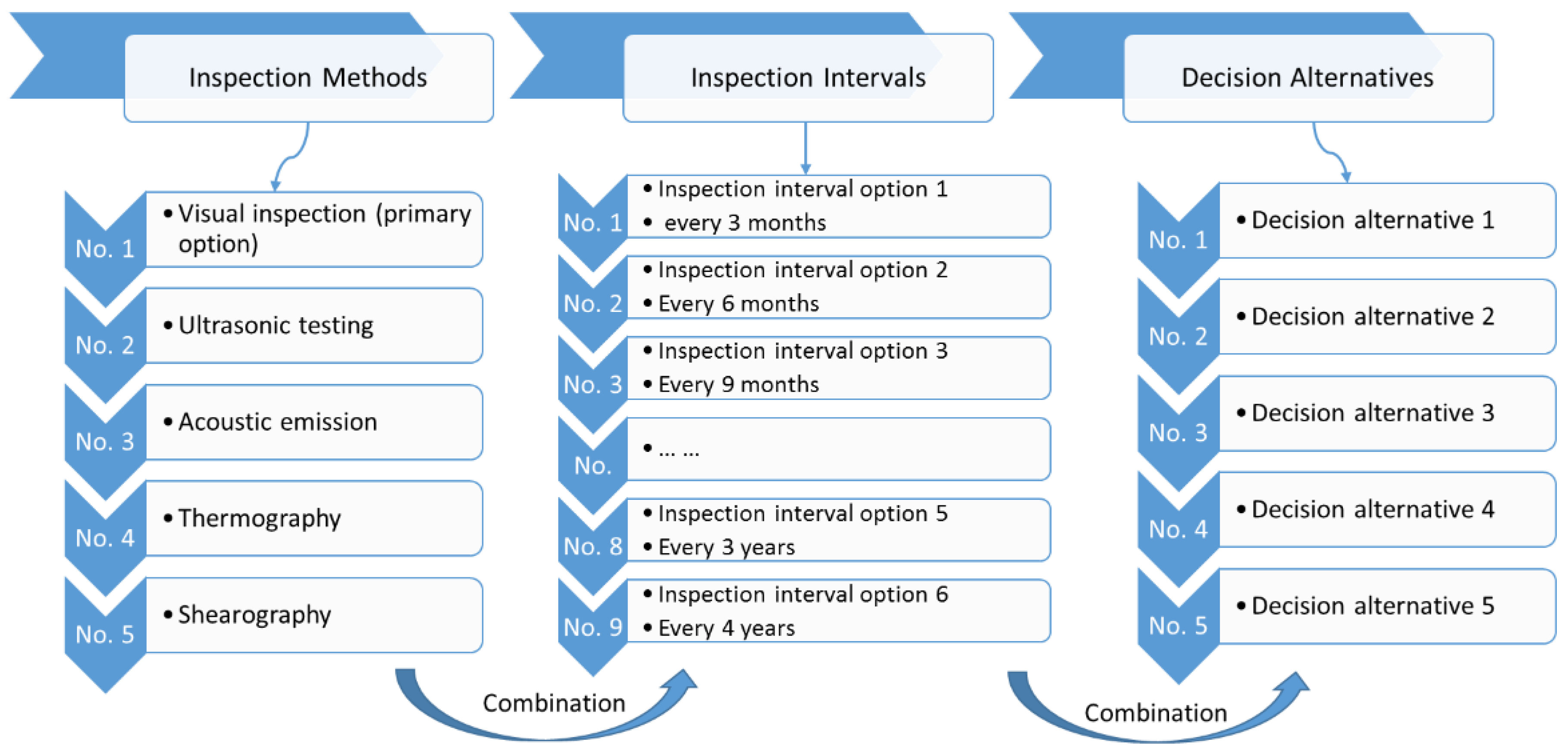
Based upon the description in Section 2.2, there are 45 combinations, or visual inspections, where nine inspection intervals and five decision alternatives are combined. For each of 45 combinations, N simulations (N = 10,000) were done, and the expected values of the total costs in the remaining lifetime were compared to find out the cost-optimal maintenance strategy.

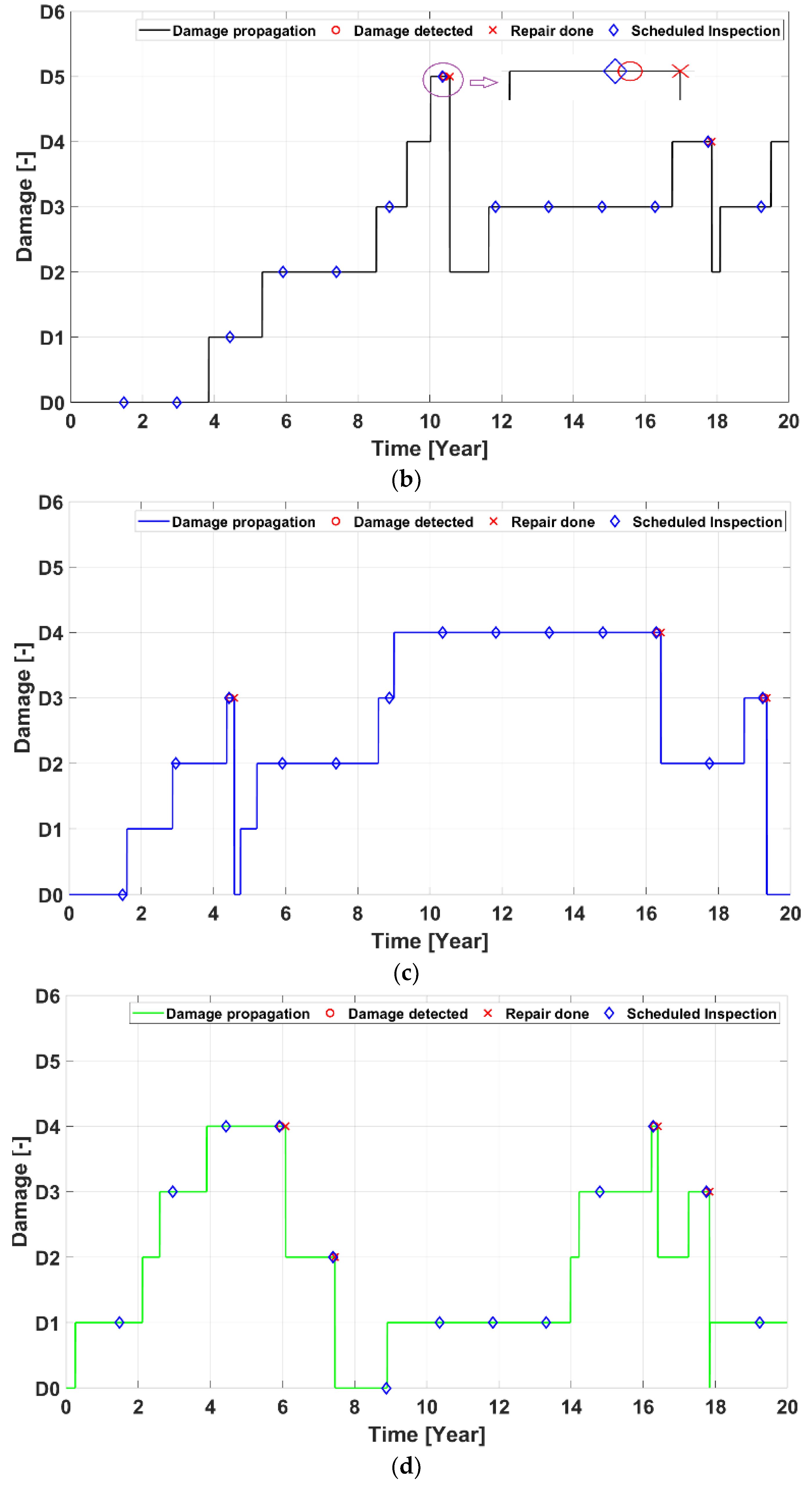
As presented in Section 4.7, the cost-optimal maintenance strategy is an inspection interval of 1.5 years and decision alternative 2. Therefore, the stochastic damage propagation corresponding to this maintenance strategy will be demonstrated in this section. Three realizations of the stochastic damage propagation for the cost-optimal maintenance strategy are shown together in Figure 4a, while Figure 4b–d separately show each of the three realizations.

The stochastic property of the discrete Markov chain model is reflected from two perspectives as summarized below:

• The sojourn time (stay duration) of each damage state (either of D1–D5) is stochastic as clearly shown in Figure 4;
• The degradation rate (namely how fast a damage propagates from one damage state to the next more severe damage state) is different in each simulation, or how fast a blade proceeds to a total collapse (namely to the damage category D6).

In Figure 4, each blue diamond represents the scheduled inspection time. Each red circle represents that an inspection is done and a damage is detected using the assumed PoDs for visual inspection as summarized in Table 6. Where a blue diamond and a red circle coincide indicates that visual inspection detects the damage at the scheduled inspection time. Otherwise, there is only one blue diamond at each scheduled inspection time. Each red cross represents that the detected damage is repaired, based upon a pre-defined decision alternative. There is a time lag between a diamond, a red circle and a red cross, which represents the repair time and also the wait time for an appropriate time window. The markers are overlapped in Figure 4, which is difficult to identify. An enlarged view is thus plotted for one inspection time in Figure 4b, where the time lag between the blue diamond and the red circle denotes the wait time for an appropriate time window and the time lag between the red circle and the red cross denotes the repair time and/or the wait time for an appropriate time window (because the repair works may be interrupted by a harsh weather condition).

After the repair is done, each line drops down to the pre-defined post-repair condition based upon the assumptions mentioned in Section 3.3. As summarized in Table 1, a decision alternative indicates a critical damage. No repair is done for detected damage that is less severe than this critical damage. For instance, it can be seen from Figure 4b–d that at some inspections no damage is detected (no red circle) and at others damage is detected and a repair is done. Based upon the assumptions regarding the post-damage condition as summarized in Table 1, the damage level drops to D0 if the damage is at either of D1, D2 or D3, or it drops to D2 if the damage is at D4 or D5. Figure 4b–d also shows that for most scheduled inspection times visual inspection cannot detect the damage, indicating that the probability of detection for smaller damage sizes is relatively low.

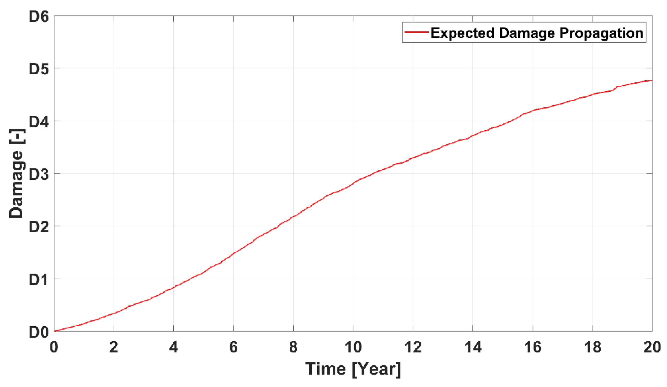
With the N realizations, the expected damage propagation is calculated, as illustrated in Figure 5.

4.7. Cost-Optimal Maintenance Strategy

The above theoretical model to calculate the maintenance costs for the different combinations of inspection intervals and decision alternatives was implemented to illustrate the procedure, see below [24].

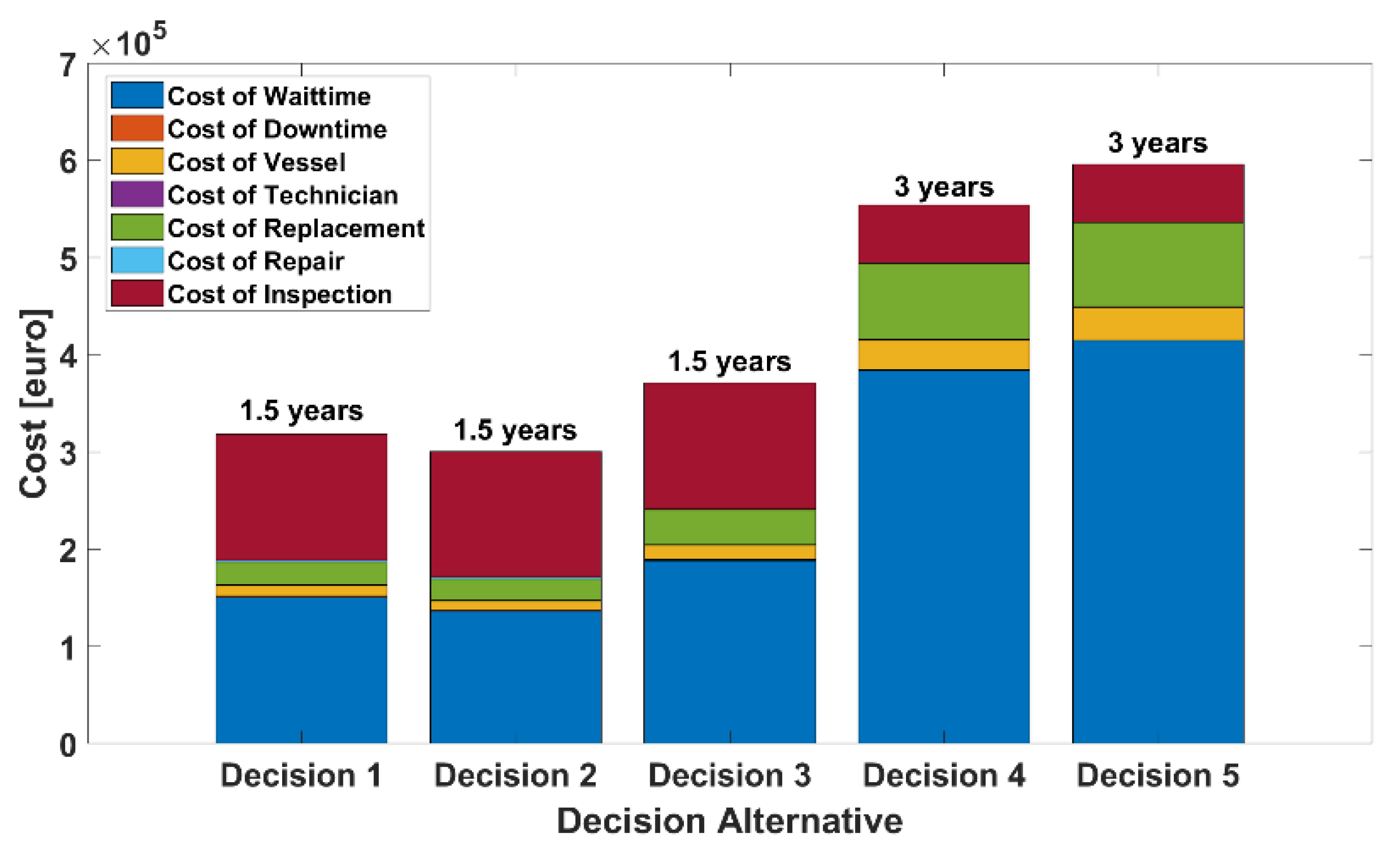
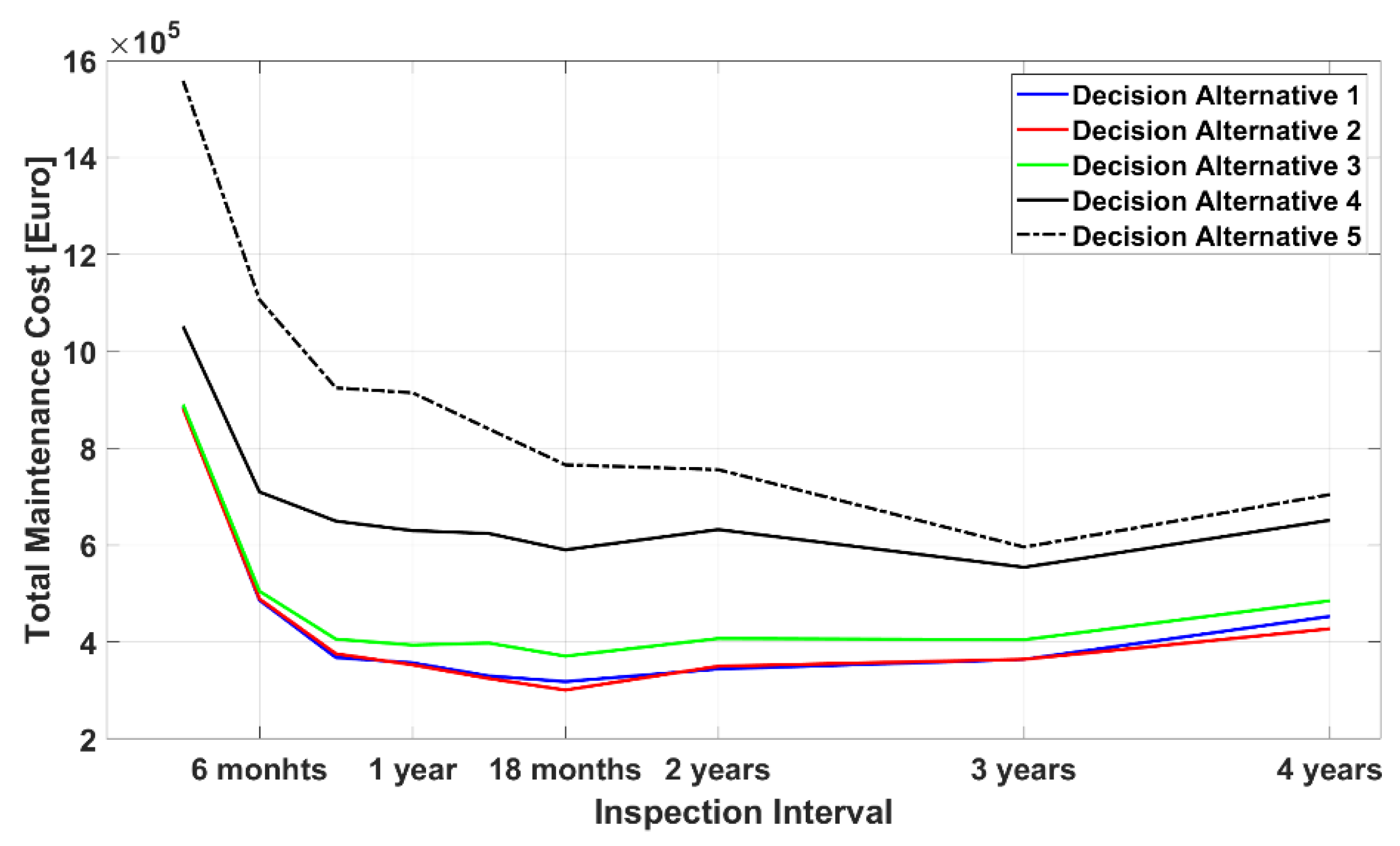
Each bar in Figure 6 shows the minimum maintenance cost corresponding to one decision alternative. The cost-optimal inspection interval for each decision alternative is marked above each bar. The cost breakdown is plotted in Figure 6. The costs due to wait time, inspection and replacement account for most of the maintenance cost. Of the 45 possible combinations, the inspection interval of 1.5 years combined with decision alternative 2 is the most cost-optimal maintenance strategy. 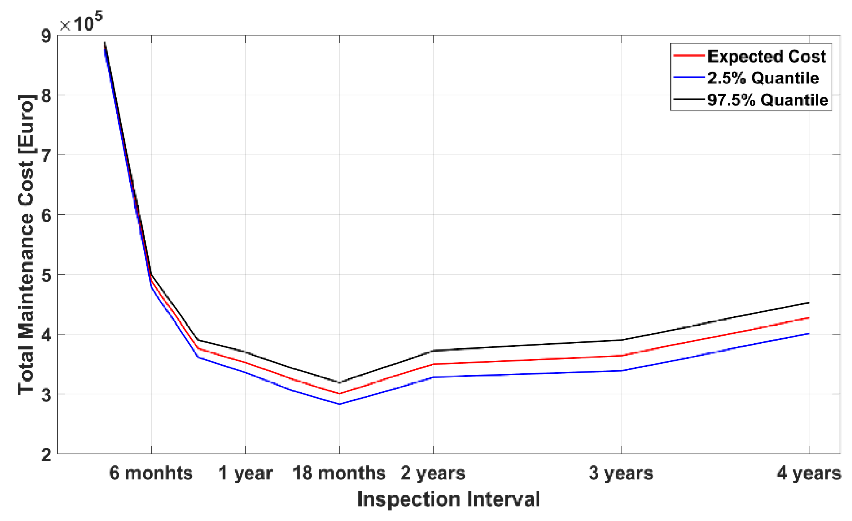The trend of the total maintenance cost as a function of inspection interval is shown for all decision alternatives in Figure 7. The 95% confidence intervals of the maintenance cost are only plotted for the cost-optimal case (the inspection interval of 1.5 years combined with decision alternative 2) to illustrate the uncertainty of the cost estimation, as shown in Figure 8. It is observed that the expected costs fluctuate between the inspection intervals of 1 year and 3 years for decision alternatives 4–5, especially the decision alternative 5. This is caused by seasonal effects combined with the simulated failure events occurring during the harsh weather conditions requiring longer waiting time to obtain an appropriate time window.

5. Conclusions and Discussion

A simulation-based method, namely combining a discrete Markov chain model with Bayesian decision tree theory, is presented in this paper in order to identify cost-optimal condition-based maintenance strategies where the cost-optimal inspection method, inspection interval, and corresponding decision alternative are identified.

The methodology is implemented and illustrated in a case study where the most cost-optimal maintenance strategy is identified in terms of an optimal inspection interval and a decision alternative. This maintenance strategy gives the 1st cost-optimal inspection time. A physical inspection can be done at this time and the inspection outcome can give some information as input to the model to determine the next cost-optimal inspection time. The procedure can proceed to determine the cost-optimal inspection intervals for the rest of the lifetime. In this case study, the in-history time series of wind speed and wave height for a specific site was used to demonstrate how the model works. For the time being, no uncertainty was assumed for the time series. However, the uncertainties associated with the weather conditions can be integrated into the model and used to quantify the influence of such uncertainties on the determination of the cost-optimal maintenance strategy.

The accuracy of the discrete Markov chain model depends upon the in-history failure records categorized based upon the six-level damage categorization scheme as mentioned in Table 1. In this sense, the information on the failure records extracted from the inspection database was used to estimate the prior transition probabilities used in this paper. When new inspections are done in the future, the failure database should be renewed and the transition probabilities updated accordingly.

The assumptions regarding the post-repair conditions were made based upon the engineering experience. A probabilistic model for simulating the post-repair conditions should be developed as the target of future research work where a more theoretically accurate model of the probabilistic damage evolution based on fracture mechanics could be integrated.

As the on-line monitoring devices are applied to monitor the deterioration process of the WT blades, plenty of information can be used as possible damage indicators. The multiple-disciplinary data-driven research methods, such as artificial intelligence and machine learning, can be used to analyze the data sets exported from the on-line monitoring devices as a promising way to make decisions on the cost-optimal maintenance strategy.