Energy Efficiency Optimization for AF Relaying with TS-SWIPT

Abstract

In this paper, we focus on energy efficiency (EE) maximization for simultaneous wireless information and power transfer (SWIPT) based energy-constrained and amplify-and-forward (AF) relay networks. We adopt low-complexity time-switching (TS) protocol to realize SWIPT at the energy-constrained relay node, and formulate an EE maximization problem in which TS factor and transmit power control are needed to be jointly optimized. Since the formulated problem is non-convex and difficult to solve, we propose an algorithm combining fractional programming and alternating convex optimization to optimize TS factor and transmit power iteratively with low complexity. Simulation results are provided to demonstrate the convergence of the proposed algorithm, as well as the performance gains in terms of EE compared with other existing schemes.

1. Introduction

Simultaneous wireless information and power transfer (SWIPT) has attracted increasing attention since it offers a great convenience to power the energy-constrained devices while maintaining the reliable communication. The idea of SWIPT is first proposed in [1], where the author assumed that the receiver is able to observe and extract power simultaneously from the same radio frequency signals. However, such assumption does not hold in practice. Motivated by this, two practical receiver protocols, namely, time-switching (TS) and power-splitting (PS), are proposed in [2,3]. For the former one, energy harvesting (EH) and information processing (IP) are switched over time, while, for the later, the received signal at receiver is split into two different power streams for EH and IP by a PS ratio.

As we all know, energy efficiency (EE), which is defined as the ratio of wireless transmit rates to the total energy consumption, is a significant metric in future networks. Much attention has been paid to the design of SWIPT based networks to obtain a high EE. In [4], the authors of investigated the EE optimization problems in the SWIPT based wireless sensor networks (WSNs), studying both the PS and TS protocols. In [5], an algorithm for EE optimization is proposed in a narrowband Multiple-Input Single-Output (MISO) system with SWIPT, where the PS protocol is considered. The authors of [6] investigated orthogonal frequency division multiple access (OFDMA) systems with PS SWIPT, and proposed a resource allocation (ResAll) scheme to maximize the EE. The EE in SWIPT based on Internet of Things (IoT) distributed antenna system (DAS) is studied in [7]. In addition, the authors of [8] investigated an energy-efficient resource management scheme in PS SWIPT based device-to-device (D2D) communication, and employed an energy-efficient stable matching algorithm to maximize the EE performance of D2D pairs and the amount of energy harvested by cellular users simultaneously. The authors of [9] designed an energy-efficient power allocation scheme to maximize the EE of the point-to-point communication system, considering the TS scheme. In [10], the authors considered a user-centric EE problem for a wireless powered communication network (WPCN), and proposed an iterative algorithm to obtain the optimal resource management policy. In [11], a ResAll strategy is investigated to maximize the EE for a radio frequency (RF) energy harvesting network, in which the TS-SWIPT enabled massive multiple-input multiple-output (MIMO) system is employed.

In a real scenario, wireless relaying has been viewed as a promising strategy for efficient information transmission by mitigating multipath fading and shadowing and increasing the diversity order [12]. Since SWIPT can provide energy to the energy-constrained relay node to encourage the relay to assist communications, the combination of SWIPT and wireless relaying has attracted a lot of interest. In [13], an optimal dynamic asymmetric power splitting (DAPS) scheme is designed to minimize the system outage probability for the amplify-and-forward (AF) relay network with SWIPT. In [14], the achievable throughput and outage probability in TS/PS scheme are evaluated for SWIPT based AF relay networks. Furthermore, in [15], a joint time allocation and power splitting (JTAPS) scheme in terms of the outage probability and ergodic capacity is studied, for a SWIPT based DF relaying network. Considering EE issues in SWIPT enabled relay communication systems, some works focus on EE maximization in two-way relay networks (TWRN) with PS-SWIPT. In [16], the authors designed an energy-efficient power allocation scheme to achieve a tradeoff between EE and spectral efficiency (SE). Considering statistical channel state information (CSI), the authors of [17] designed a statistical EE model, where EE is maximized under the constraints on the total transmit rate and power, respectively. The authors of [18] extended the scenario to MIMO systems.

However, TWRN is not always more energy-efficient than one-way relay networks (OWRN) [19]; together with the difficulty in self-interference cancellation in TWRN, some works turn to the EE design in SWIPT enabled OWRN with PS protocol. In [20], the authors of investigated a one-way SWIPT network consisting of multiple sources, destinations and energy-constrained relays, where a joint ResAll and relay selection scheme is designed to maximize the system EE. The authors of [21] considered a SWIPT enabled OWRN under DF mode, where power allocation is optimized to maximize the EE of the system, with constraints on PS factor and the source node’s transmit power. However, there are some limits in [20,21]. In [20], the optimal PS factor is obtained by global search, leading to a high computational complexity. In [21], the PS factor is fixed to obtain the optimal transmit power, which is not in accordance with actual scenarios and the performance gain is limited. In addition, because of the decoding and re-encoding operations in DF relaying mode nodes, a higher complexity is also required.

In this paper, we investigate EE optimization for SWIPT enabled one-way AF relay networks based on low-complexity TS protocol. (Note that we only provide the theoretical analysis and simulation for performance evaluation in this work due to the hardness of implementation in the real application and our limited resources.) We formulate an EE maximization problem, where transmit power control and TS factor allocation are jointly optimized to obtain more performance gains. As the problem is non-convex, we first transform it into a convex optimization problem resorting to fractional programming, which is then solved by a low-complexity iterative algorithm based on alternating convex optimization.

The rest of this paper is structured as follows. The system model is provided in Section 2. In Section 3, we formulate the optimization problem to maximize the EE of the considered system and design an optimal scheme to obtain the optimal solutions. Numerical results are provided in Section 4, followed by conclusions in Section 5.

2. System Model

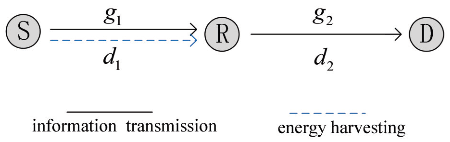
In this work, we consider an AF one-way SWIPT enabled relaying network, and the TS method is employed to achieve SWIPT. As illustrated in Figure 1, there are three nodes, where S and D are source node and destination node, respectively, and R denotes an energy-constrained relay node in AF mode, which is the intermediary to assist the transmission between S and D. Assume that there is a single antenna equipped at each node, and that there is no direct link between S and D due to severe path loss and shadowing [12]. Let $d_1$ (or $d_2$) denote the distance between S (or D) and R. Let $g_1$ and $g_2$ represent the S-R and R-D channels, respectively. Assume that all channels obey frequency nonselective Rayleigh block fading and are reciprocal. Then, the path loss model is given by $g_i{d}_i^{-p}$ ($i=1\mathrm{or}2$), where p is the path loss exponent. Meanwhile, the CSI at receiver is assumed to be available.

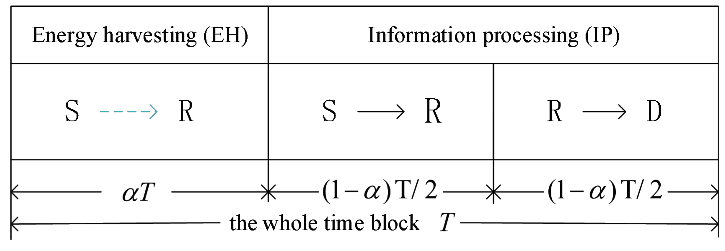
The whole transmission block can be divided into three parts, as shown in Figure 2. Let T and $\alpha \in (0,1)$ denote the whole symbol duration and the TS factor, respectively. R scavenges energy from the radio frequency signal received from source node S during $\alpha T$. The half of $(1-\alpha )T$ is spent on signal transmission from S to R. Then, R forwards the processed signal to D at the remaining $\frac{(1-\alpha )}{2}T$. Note that all the energy harvested at R is consumed for forwarding source information to D.

At the EH phase, S sends the source signal to R, and R harvests energy by an EH receiver. Then, the RF signal received at R can be expressed as

$$\begin{array}{c}\hfill y_r(t)=\sqrt{P_t}\frac{g_1}{\sqrt{d_1^p}}s(t)+n_r(t),\end{array}$$

(1)

where $P_t$ denotes the transmission power at S, $n_r\sim CN(0,{\sigma }_r^2)$ is the additive white Gaussian noise (AWGN) at R caused by receiver antenna, $s(t)$ is the normalized source signal with $E\left\{{\left|s(t)\right|}^2\right\}=1$, and $E\left\{·\right\}$ is the expectation operator.

Based on Equation (1), the harvested energy at R during $\alpha T$ is given by

$$\begin{array}{c}\hfill E=\alpha T\eta P_t\frac{{\left|g_1\right|}^2}{d_1^p},\end{array}$$

(2)

where $0<\eta <1$ is the energy conversion efficiency.

Then, at the first half of the rest time, $(1-\alpha )T/2$, the RF signal at relay R received from S is converted into a sampled signal by the information receiver of R, which is given as

$$\begin{array}{c}\hfill y_r(n)=\sqrt{P_t}\frac{g_1}{\sqrt{d_1^p}}s(n)+n_r(n)+n_c(n),\end{array}$$

(3)

where n is the symbol index, and $n_c\sim CN(0,{\sigma }_c^2)$ is the sampled AWGN due to signal conversion from RF band to baseband.

Based on Equation (2), the transmission power from R is given by

$$\begin{array}{c}\hfill P_r=\frac{E}{(1-\alpha )T/2}=\frac{2\eta P_t{\left|g_1\right|}^2\alpha }{d_1^p(1-\alpha )},\end{array}$$

(4)

where $(1-\alpha )T/2$ is the time that R takes to forward source signal to destination.

At the remaining half of the rest time $(1-\alpha )T$, R amplifies the signal $y_r(n)$ and forwards it to destination D. Then, the received signal at D is

$$\begin{array}{c}\hfill y_d(n)=\frac{g_2}{\sqrt{d_2^p}}\beta y_r(n)+n_d(n),\end{array}$$

(5)

where $n_d\sim CN(0,{\sigma }_d^2)$ is the AWGN at D, and $\beta =\sqrt{\frac{P_r}{P_t\frac{{\left|g_1\right|}^2}{d_1^p}+{\sigma }_r^2+{\sigma }_c^2}}$ is the amplifier factor due to the AF method employed at R.

By substituting Equations (3) and (4) into Equation (5), we have

$$\begin{array}{c}\hfill \begin{array}{c}{y}_d(n)=\underset{\mathrm{signal}}{\underbrace{\frac{\sqrt{2\eta \alpha }{P}_t{\left|g_1\right|}^2{g}_2}{\sqrt{(1-\alpha )d_1^p{d}_2^p}\sqrt{P_t{\left|g_1\right|}^2+d_1^p{\sigma }_{rc}^2}}s(n)}}+\underset{\mathrm{overallnoise}}{\underbrace{\frac{\sqrt{2\eta \alpha P_t}{g}_1{g}_2}{\sqrt{(1-\alpha )d_2^p}\sqrt{P_t{\left|g_1\right|}^2+d_1^p{\sigma }_{rc}^2}}{n}_{rc}(n)+n_d(n)}},\end{array}\end{array}$$

(6)

where ${\sigma }_{rc}^2\stackrel{\Delta }{=}{\sigma }_r^2+{\sigma }_c^2$ and $n_{rc}(n)\stackrel{\Delta }{=}{n}_r(n)+n_c(n)$.

Thus, from Equation (6), the signal-to-noise ratio (SNR) at D can be calculated as

$$\begin{array}{c}\hfill {\gamma }_D=\frac{\frac{2\eta \alpha P_t^2{\left|g_1\right|}^4{\left|g_2\right|}^2}{(1-\alpha )d_1^p{d}_2^p(P_t{\left|g_1\right|}^2+d_1^p{\sigma }_{rc}^2)}}{\frac{2\eta P_t\alpha {\left|g_1\right|}^2{\left|g_2\right|}^2{\sigma }_{rc}^2}{(1-\alpha )d_2^p(P_t{\left|g_1\right|}^2+d_1^p{\sigma }_{rc}^2)}+{\sigma }_d^2}=\frac{2\eta P_t^2{\left|g_1\right|}^4{\left|g_2\right|}^2\alpha }{2\eta P_t{\left|g_1\right|}^2{\left|g_2\right|}^2{d}_1^p{\sigma }_{rc}^2\alpha +(1-\alpha )P_t{\left|g_1\right|}^2{d}_1^p{d}_2^p{\sigma }_d^2+(1-\alpha )d_1^{2p}{d}_2^p{\sigma }_{rc}^2{\sigma }_d^2}.\end{array}$$

(7)

Further, the achievable bits of the system can be written as

$$\begin{array}{c}\hfill R_{\mathrm{EE}}=\frac{(1-\alpha )T}{2}{log}_2(1+{\gamma }_D).\end{array}$$

(8)

The total energy consumption is expressed as

$$\begin{array}{c}\hfill P_{\mathrm{TOT}}=(\alpha T+\frac{(1-\alpha )T}{2})P_t/\epsilon +P_{C}T,\end{array}$$

(9)

where $\epsilon$ and $P_C$ denote the power amplifier efficiency of S and circuit power consumption, respectively.

3. Problem Formulation and Solution

The energy efficiency is defined as the ratio of the achievable bits to the total energy consumption of the system, which is written as

$$\begin{array}{c}\hfill {\eta }_{\mathrm{EE}}=\frac{R_{\mathrm{EE}}}{P_{\mathrm{TOT}}}=\frac{\frac{(1-\alpha )}{2}{log}_2(1+\frac{2\eta P_t^2{\left|g_1\right|}^4{\left|g_2\right|}^2\alpha }{2\eta P_t{\left|g_1\right|}^2{\left|g_2\right|}^2{d}_1^p{\sigma }_{rc}^2\alpha +(1-\alpha )P_t{\left|g_1\right|}^2{d}_1^p{d}_2^p{\sigma }_d^2+(1-\alpha )d_1^{2p}{d}_2^p{\sigma }_{rc}^2{\sigma }_d^2})}{(\frac{(1+\alpha )}{2})P_t/\epsilon +P_C}.\end{array}$$

(10)

Based on the above analysis, the EE optimization problem can be formulated as

$$\begin{array}{c}\hfill \begin{array}{c}(\mathrm{P}1):\underset{P_t,\alpha }{max}{\eta }_{\mathrm{EE}}\hfill \\ \mathrm{s}.\mathrm{t}.0<P_t<P_{max}\hfill \\ 0<\alpha <1\hfill \end{array},\end{array}$$

(11)

where the first constraint means the transmit power at source node is limited by the maximum transmit power $P_{max}$.

Note that P1 is a non-convex fractional optimization problem and is difficult to solve. Let $q^{*}$ denote the maximum EE of the investigated system. Then, we have

$$\begin{array}{c}\hfill q^{*}=\frac{R({P_t}^{*},{\alpha }^{*})}{P({P_t}^{*},{\alpha }^{*})}=\underset{P_t,\alpha }{max}\frac{R(P_t,\alpha )}{P(P_t,\alpha )}\end{array}$$

(12)

where ${P_t}^{*}$ and ${\alpha }^{*}$ denote the optimal transmission power and TS factor, respectively.

Motivated by the Dinkelbach’s method [22], Lemma 1 is provided to transform P1 to a tractable problem as follows.

Lemma 1.

The maximum EE $q^{*}$ is achieved if and only if the following equation is satisfied.

$$\begin{array}{c}\hfill \begin{array}{c}\underset{P_t,\alpha }{max}R(P_t,\alpha )-q^{*}P(P_t,\alpha )\hfill \\ =R(P_t^{*},{\alpha }^{*})-q^{*}P(P_t^{*},{\alpha }^{*})=0.\hfill \end{array}\end{array}$$

(13)

For $R(P_t,\alpha )>0$ and $P(P_t,\alpha )>0$, Lemma 1 can be proved in Appendix A by a similar way as in [22].

Based on Lemma 1, we propose a Dinkelbach based iteration algorithm, as shown in Algorithm 1, to obtain the optimal solution to P1. As shown in Algorithm 1, the algorithm will converge to the optimal energy efficiency $q^{*}$, which is verified in Appendix B.

In each iteration, we have to solve the inner problem for a given parameter q, as

$$\begin{array}{c}\hfill \begin{array}{c}(\mathrm{P}2):\underset{\alpha ,P_t}{max}F(\alpha ,P_t)=R(\alpha ,P_t)-qP(\alpha ,P_t)\hfill \\ \mathrm{s}.\mathrm{t}.0<P_t<P_{max}\hfill \\ 0<\alpha <1\hfill \end{array}.\end{array}$$

(14)

Let $({\alpha }^{\prime },P_t^{\prime })$ be the optimal solution to P2. With a given error tolerance $\zeta$, when $R({\alpha }^{\prime },P_t^{\prime })-$$qP({\alpha }^{\prime },P_t^{\prime })<\zeta$ holds, the optimal solution to P1 can be obtained.

We can notice that the main challenge in Algorithm 1 is solving the non-convex problem P2. The following part is devoted to solving P2.

Proposition 1.

With a given $P_t$, P2 is a convex problem with regard to α. Similarly, when α is given, P2 is a convex problem with regard to $P_t$.

Proof. 

See Appendix C. □

Algorithm 1 The proposed Dinkelbach based iteration algorithm to maximize EE.

1: Setting: $\eta$, $P_t$, ${\sigma }^2$, $d_1$, $d_2$, and p 2: Inputting:        the instantaneous CSI, $g_1$ and $g_2$ 3: Initialization:        the iteration index $s=1$, $q=0$, the maximum number of iterations $I_{max}$, and the maximum tolerance $\zeta$ 4: Repeat: 5: Solve the problem (P2) in Equation (14) for a given q, and obtain resource allocation policies $\left\{{P_t}^{\prime },{\alpha }^{\prime }\right\}$ 6: If $R({\alpha }^{\prime },P_t^{\prime })-qP({\alpha }^{\prime },P_t^{\prime })<\zeta$, then 7: Convergence = true 8: Return $\left\{{\alpha }^{*},{P_t}^{*}\right\}=\left\{{\alpha }^{\prime },{P_t}^{\prime }\right\}$ and $q^{*}=\frac{R({\alpha }^{\prime },{P_t}^{\prime })}{P({\alpha }^{\prime },{P_t}^{\prime })}$ 9: Else 10: Set $q=\frac{R({\alpha }^{\prime },{P_t}^{\prime })}{P({\alpha }^{\prime },{P_t}^{\prime })}$ and $s=s+1$ 11: Convergence = false 12: End if 13: Until Convergence = true or $s=I_{max}$

According to Proposition 1, we further propose an alternating power and time allocation algorithm algorithm based on the alternating convex optimization (ACO) method to obtain the optimal solution to P2, as shown in Algorithm 2. Let i be the iteration index. There are two major steps in the ith iteration: one is updating the transmit power ${P_t}^{i+1}$ with a fixed time-switching factor ${\alpha }^i$, and the other is updating ${\alpha }^{i+1}$ for a fixed ${P_t}^{i+1}$. This process will continue until the stop condition $\left|F({P_t}^{i+1},{\alpha }^{i+1})-F({P_t}^{i+1},{\alpha }^i)\right|<\varsigma$ is satisfied, where $\varsigma$ denotes the maximum tolerance. Then, the optimal solution to P2 $({P_t}^{\prime },{\alpha }^{\prime })$ is obtained by letting ${P_t}^{\prime }={P_t}^{i+1},{\alpha }^{\prime }={\alpha }^{i+1}$.

Algorithm 2 The proposed alternating power and time allocation algorithm to solve P2.

1: Setting: $\eta$, $P_t$, ${\sigma }^2$, $d_1$, $d_2$, and p 2: Inputting:        the instantaneous CSI, $g_1$ and $g_2$ 3: Initialization:        the iteration index $i=1$, ${\alpha }^1=0.5$, the maximum number of iterations $I_m$ and the maximum tolerance $\varsigma$ 4: Optimization: 5: Solve (P2) with a given ${\alpha }^i$ and obtain power allocation ${P_t}^{i+1}$ 6: Obtain $F({P_t}^{i+1},{\alpha }^i)$ 7: Solve (P2) with a given ${P_t}^{i+1}$ and obtain time allocation ${\alpha }^{i+1}$ 8: Obtain $F({P_t}^{i+1},{\alpha }^{i+1})$ 9: If $\left|F({P_t}^{i+1},{\alpha }^{i+1})-F({P_t}^{i+1},{\alpha }^i)\right|<\varsigma$, then 10: Flag = 1, set ${P_t}^{\prime }={P_t}^{i+1}$, ${\alpha }^{\prime }={\alpha }^{i+1}$ and return 11: Else 12: Set $i=i+1$ 13: Flag = 0 14: End if 15: Until flag = 1 or $i=I_m$

By integrating Algorithm 2 into Step 5 of Algorithm 1, the optimal solution for P1 can be obtained. We verified the quick convergence of the proposed Algorithms 1 and 2 in the simulations.

4. Simulation Results

In this section, numerical results are provided to evaluate the performance of the proposed optimal scheme. To verify the advantages of the proposed scheme, we compared our proposed scheme with three other schemes: (1) the optimal EE scheme with a fixed TS factor; (2) the optimal EE scheme with a fixed transmit power of the source; and (3) the EE of the SE optimal scheme [23]. Unless otherwise specified, the simulation parameters used were set as follows: [14,16]: $\eta =0.8$, $p=3$, ${\mathrm{P}}_C=0.1$ W, $\epsilon =0.38$, ${\mathrm{P}}_{\mathrm{t}}=1$ W, $P_{max}=1$ W, $d_1=d_2=1.2$ m, ${\sigma }_{rc}^2={\sigma }_d^2=0.01$.

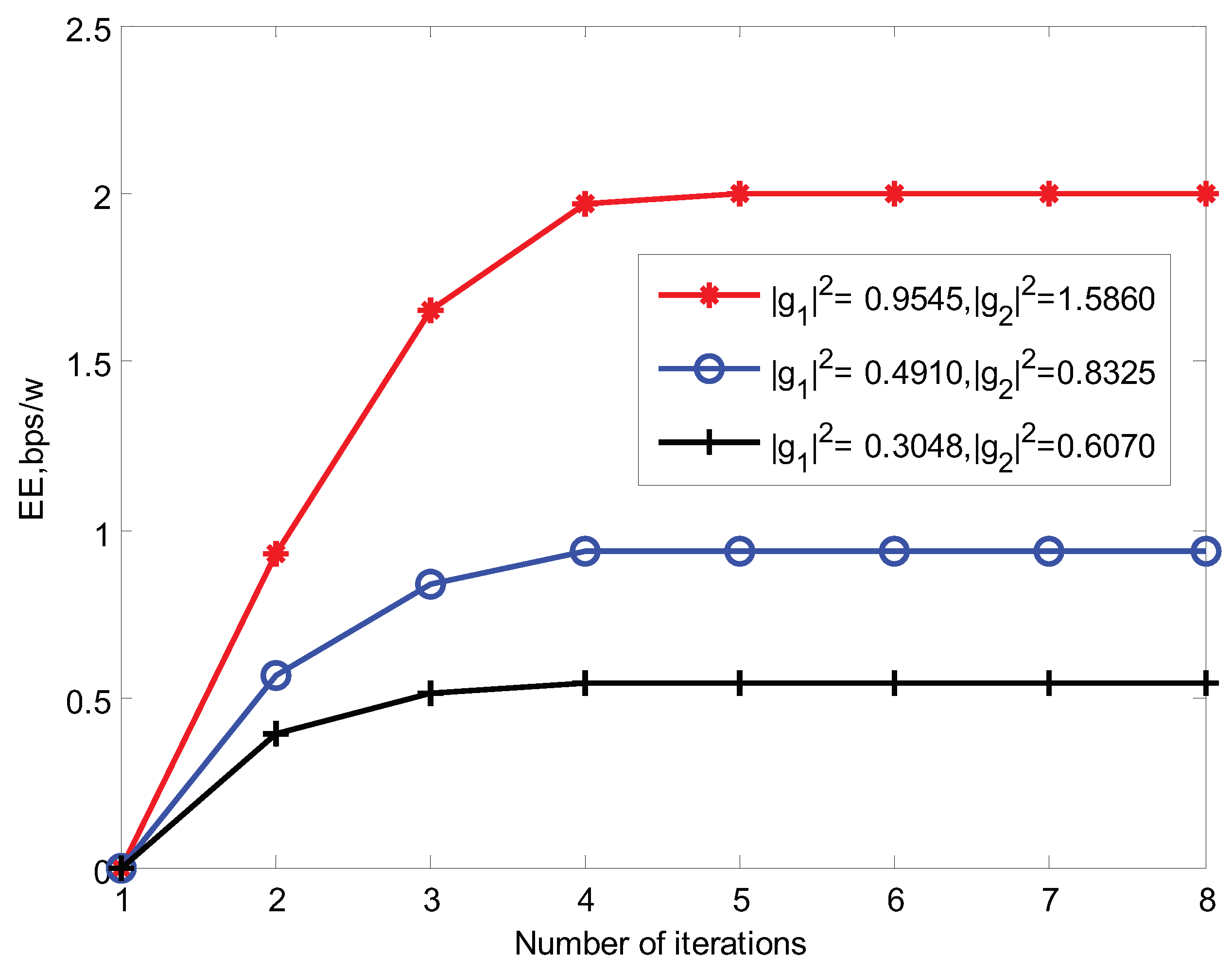
In Figure 3, the behavior of the EE versus number of iterations is plotted under three different settings of channel gains. (Note that the proposed algorithms are independent to the channel fading. Once the CSI is available, our proposed algorithms are also useful. In simulations, we considered the Rayleigh fading channel. This is because the Rayleigh fading channel is the special case of the generalized $\kappa -\mu$ fading channel [24,25], when $\kappa \to 0$ and $\mu =1$.) It can be observed that Algorithm 1 converged within limited iteration numbers (i.e., fewer than five iterations), which illustrates the effectiveness of the proposed Algorithm 1.

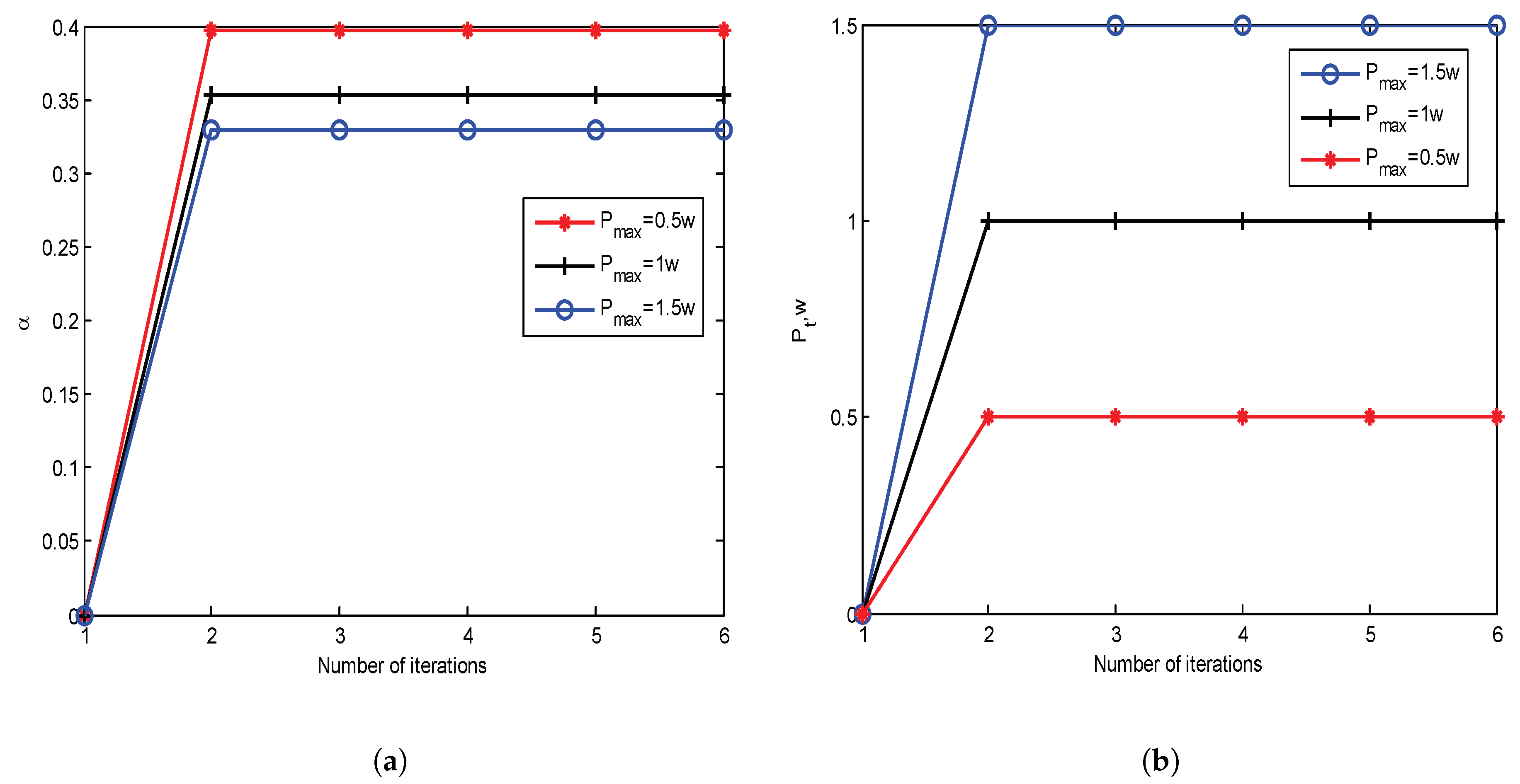
Figure 4 demonstrate the convergence of Algorithm 2. Figure 4a shows the TS factor against iteration number for different values of $P_{max}$, while Figure 4b illustrates transmission power of the source against iteration number. It can be seen that both the TS factor and the transmission power of the source always converged within two iterations. Thus, Algorithm 2 is convergent.

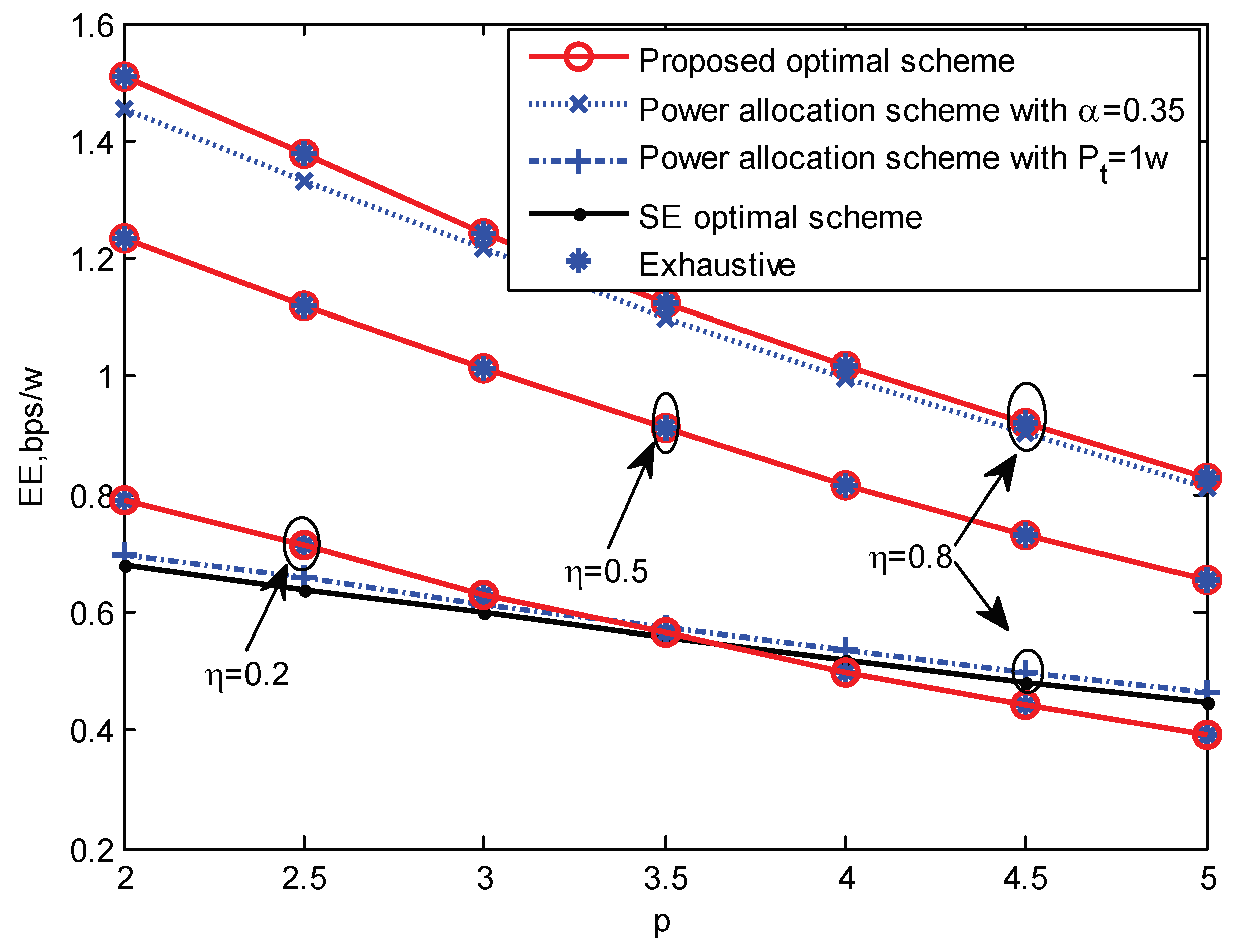
Since the path loss factor and the energy conversion efficiency can affect the EE, Figure 5 shows the EE versus the path loss factor p for different values of energy conversion efficiency $\eta$. The schemes with a fixed TS factor, with a fixed transmit power of source and with the optimal SE were compared with our proposed optimal scheme. As shown in Figure 5, the curve was monotonously decreasing for a specific value of the energy conversion efficiency $\eta$. It was also observed that the system EE for a larger energy conversion efficiency $\eta$ outperformed that for a smaller one when the pass loss factor p was fixed because the higher was the energy conversion efficiency $\eta$, the more energy was harvested at the relay, resulting in a higher EE. Additionally, one can see that the result obtained by our proposed scheme matched with the result by the exhaustive search method, which indicates high accuracy of our proposed algorithms. One can also observe that our proposed scheme outperformed all other considered schemes in terms of EE. Specifically, by comparing with the scheme with a fixed transmit power of the source and the scheme of the optimal SE, the EE of our proposed scheme was double. For example, when $p=3$ and $\eta =0.8$, the EE of the scheme with a fixed transmit power of source and the scheme of the optimal SE were about 0.7 bps/w, while the EE of our proposed scheme reached 1.4 bps/w.

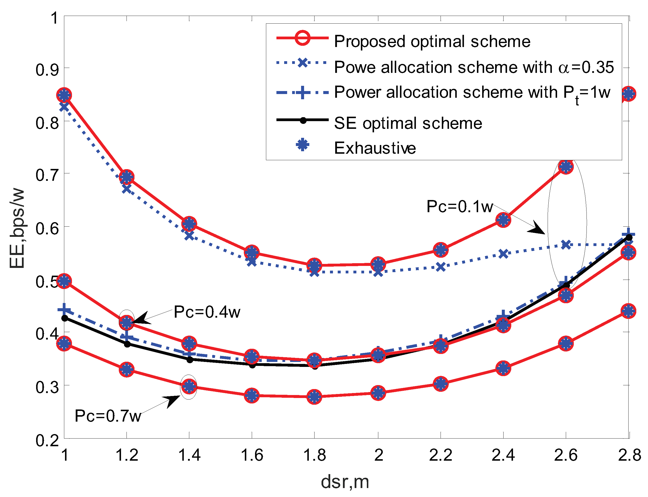
Figure 6 illustrates the EE versus the source-relay distance with different settings of circuit power consumption, which also contrasts our proposed optimal scheme with the schemes with a fixed TS factor, with a fixed transmit power of source and with the optimal SE. It can be seen that, for a specific circuit power consumption, with the increasing of the source-relay distance, the EE of the proposed scheme decreased at first, reached the minimum value and then increased. In particular, when the source-relay distance was about 1.8 m, the minimum EE was obtained. The reason is as follows. The relay harvested less energy from the RF signal of the source at EH phase as the distance between source and relay increased. Accordingly, the transmit power of the relay was reduced, which brought the lower achievable bits of the system, thus the EE decreased. However, as the relay moved closer to the destination, it spent less time forwarding signal to destination. For the specific energy harvested at relay, it could achieve more transmission of bits. Correspondingly, the EE of the system improved. This finding suggests that, in such scenario as we considered, to meet a higher EE, we should put the relay as close as possible to the source or destination node. Besides, it can also be noticed that less circuit power consumption of the system led to higher EE. This is because less circuit power consumption led to less energy consumption for the whole transmission, inferring that more energy would be used to forward and a higher EE could be achieved. We similarly found that our proposed scheme was more energy efficient than the three other schemes, as expected. The result obtained by our proposed scheme and the result by the exhaustive search method closely coincide, which further demonstrates the validity of our proposed algorithms.

5. Conclusions

In this paper, we have studied the EE of a SWIPT based AF relay network. We have focused on the joint optimization of transmit power control and TS factor allocation in order to maximize the EE of the system, and low-complexity iterative algorithms have been proposed based on fractional programming and alternating convex optimization to obtain the optimal solutions. Simulation results have verified the convergence of the proposed iterative algorithm, and have demonstrated the effectiveness of our proposed algorithms by comparing with the optimal EE scheme with a fixed TS factor algorithm, the optimal EE scheme with a fixed transmit power algorithm, and the EE of the SE optimal algorithm. Next, we present our future research directions. Firstly, we will extend our work to the PS-SWIPT enabled AF relay network and focus on the design of the transmit power and PS ratio to achieve the maximum EE of the system. Secondly, we will further include the non-linear EH model into our work to be more practical.