Article

Modelling of Electrically-Assisted Turbocharger Compressor Performance

by
Mamdouh Alshammari
,
Nikolaos Xypolitas
and
Apostolos Pesyridis
*
College of Engineering and Design, Brunel University London, Uxbridge UB8, UK
*
Author to whom correspondence should be addressed.
Energies 2019, 12(6), 975; https://doi.org/10.3390/en12060975
Submission received: 25 January 2019 / Revised: 7 March 2019 / Accepted: 8 March 2019 / Published: 13 March 2019

Abstract

:
For the purposes of design of a turbocharger centrifugal compressor, a one-dimensional modelling method has been developed and applied specifically to electrically-assisted turbochargers (EAT). For this purpose, a mix of authoritative loss models was applied to determine the compressor losses. Furthermore, an engine equipped with an electrically-assisted turbocharger was modelled using commercial engine simulation software (GT-Power) to assess the performance of the engine equipped with the designed compressor. A commercial 1.5 L gasoline, in-line, 3-cylinder engine was selected for modeling. In addition, the simulations have been performed for an engine speed range between 1000 and 5000 rpm. The design target was an electric turbocharger compressor that could meet the boosting requirements of the engine with noticeable improvement in a transient response. The results from the simulations indicated that the EAT improved the overall performance of the engine when compared to the equivalent conventional turbocharged engine model. Moreover, the electrically-assisted turbochargers (EAT) equipped engine with power outputs of 1 kW and 5 kW EAT was increased by an average of 5.96% and 15.4%, respectively. This ranged from 1000 rpm to 3000 rpm engine speed. For the EAT model of 1 kW and 5 kW, the overall net reduction of the BSFC was 0.53% and 1.45%, respectively, from the initial baseline engine model.

1. Introduction

1.1. General Turbocharging Advantages and Limitations

The impact of global warming has forced regulatory authorities around the world to establish strict regulations on CO2 emissions and other greenhouse gas emissions. Although the regulations created several technical challenges for the automotive industry, this led to technology development since there was a demand of decreasing the fuel consumption of engines. This also led to increasing their performance because more power and more sustainable products had to be designed to reduce their environmental impact [1,2,3]. Among various technologies that have been developed, the most effective way to increase the fuel economy and decrease the CO2 emissions of passenger vehicles is engine downsizing [4,5]. The purpose of engine downsizing is the reduction of the throttling and friction losses associated with a larger engine by using a smaller, high power-density engine. Thus, engine efficiency is improved by operating in the more efficient regions, with the boosting device (turbocharger or supercharger) being the crucial component that allows this significantly increased power density to occur.
However, these conventional boosting devices have some limitations. Traditionally, the main drawback of the turbocharger is the delay in generating boost pressure, which results in insufficient torque at low engine speeds, known as turbo lag [1,6]. Conversely, the mechanical supercharger has a fast response at a low engine speed, but it creates parasitic losses to the engine since the required power for its operation is taken from the engine. One feasible solution for avoiding the drawbacks of the conventional boosting technologies is the electrification of the boosting system [7,8]. Electrification systems reduce the transient response (turbo lag) by 50% to 400% with respect to time-to-torque, which depend on the operating point of the turbocharger and engine. In addition, they can increase the overall engine efficiency for a substantial part of the turbocharged-engine operating range when compared to equivalent mechanical turbocharger systems [9,10]. Therefore, the aim of the paper is to model an advanced electric turbocharger compressor to improve the transient response of the turbocharger at low engine speed and, in turn, to enhance the performance, efficiency, and fuel economy of the engine.

1.2. Electrically Assisted Turbocharger (EAT)

Katrasnik et al. [11] evaluated the electrical assisted turbocharger in which the torque is applied to the turbocharger using a high speed electric motor. The motor can be integrated into the turbocharger bearing housing or as an extension to the turbocharger shaft on the compressor side. On the other hand, Baines [12] claimed this type of arrangement would be a less severe working environment for the motor than that of the electrically driven compressor in a combined charging system. However, the unit size will be increased and the effects on the shaft dynamics could be problematic. Generally, more weight will be added by the motor, which will affect bearing loads, and will increase the base inertia of the turbocharger. Nonetheless, the motor can be operated as a generator to recover the exhaust energy as electric power, which is an additional feature. Katrasnik et al. [11] conducted an experiment in which the transient response and load acceptance of a 6.9 L cylinder commercial diesel engine were simulated with the original fixed geometry turbocharger installed and also with two electrically assisted variants. After collaborating and validating the engine model with the experiment data, the transient response of the engine at a fixed speed tip-in was decreased by up to 55% with an electrically-assisted turbocharger. The acceptance load was then developed.

1.3. Preliminary Design of Centrifugal Compressors

Yang et al. [7] developed a radial compressor for an electric supercharger in a 2.0 L petrol engine by using a mean-line design process. In the process, the operating conditions of the compressor were provided and a set of geometrical parameters were selected to start the design. Then, computational fluid dynamics (CFD) simulation was applied in a detailed 3D design to analyze the compressor’s performance. The results of the computational fluid dynamics (CFD) simulation method showed a moderate reduction in total pressure ratio and total impeller efficiency when compared to the predicted corresponding values in the mean line method. However, it is worth noting that the scroll was excluded in the computational fluid dynamics (CFD) simulation. Hence, in this method, the predicted values of the total pressure ratio and total efficiency were slightly increased since the scroll loss was not included. Therefore, there is a significant difference in the results obtained from 1D modelling method and the computational fluid dynamics (CFD) simulation.
On the other hand, Harley et al. [13] developed a novel mean line modelling method for radial compressors that is applied in automotive turbochargers. In this modelling approach, the pressure ratio and the recirculation flow of the compressor are linked. Furthermore, Harley et al. [13] stated that the results obtained from the existing mean line methods would not be accurate in comparison with test data since the pressure ratio is predicted and, thus, it could rise and lead to surge. However, the new method deals with the issue by modelling the recirculation effects. Three different diameter centrifugal compressors with vane-less diffusers and scroll collectors were used for the process [13]. The procedure starts with the analysis of the inlet blockage creation by recirculation flow and how this affects the induced flow into the impeller. The Galvas [14] loss model collection was selected for the analysis. According to Harley et al. [13,15,16], not only is it a robust model, but it also operates best across a variety of automotive turbocharger radial designs. Then, computational fluid dynamics (CFD) modelling was applied to verify all the results. The results indicate that, with the proposed mean line modelling process, the prediction methods are improved when the flow conditions are represented more accurately in the impeller. A major positive outcome of this study is that the novel method could be used for any centrifugal compressor to improve the blade angle selection when recirculation occurs.
For further validation and exposing the weakness of the novel mean line modelling method, another experiment was performed by Harley et al. [7]. Although the modelling process was for the same variety of the turbocharger, automotive, the investigation was done on two new centrifugal compressors. For the purpose of this study, mean line modelling was used.
On the one hand, the results obtained from the single-zone modelling process were predicted accurately for the larger compressor at low-to-medium tip speeds. However, there was a slight difference in the prediction at the highest tip speeds. Moreover, the results obtained from the smaller compressor were not predicted accurately since the characteristic of the pressure ratio was insufficient toward the surge. As far as the single passage computational fluid dynamics (CFD) method is concerned, the results have shown that the inlet circulation can be predicted with high accuracy. However, the method is incapable of predicting the performance in the impeller trailing edge [7].
In a recent paper by Samkit et al. [17], the preliminary design of a centrifugal compressor was investigated using a non-dimensional method. The parameters’ dimensions were calculated by various equations and correlations such as Weisner, Lame Ovals equations, Rodger and Sapiro [9], and Johnston and Dean [18] correlations. Moreover, a 3D centrifugal compressor was designed to validate the results of the theoretical analysis. The analysis and simulations indicated that there was a slight difference, about 9% in the results between CFD and the theoretical method. Although the obtained results were in good agreement, the design losses were neglected from the theoretical calculations. Thus, the preliminary design procedure of the radial compressor is not accurate enough since the variation in the results would increase if the design losses were included.
Kerres et al. [19] compared the performance of two types of 1D prediction models with numerical data for an automotive turbocharger centrifugal compressor with a vaneless diffuser and a scroll (Figure 1). The prediction models used for the comparison were suggested by Aungier [20] and Oh et al. [21]. Moreover, the numerical results obtained by a 3D Reynolds-averaged Navier–Stokes (RANS) simulation for a small turbocharger compressor. The results of the comparison indicated that the 1D model were less accurate at low impeller speeds and choke than the computational fluid dynamics (CFD) 3D method. However, at high impeller speeds, they could predict precisely with a slight variation from the predictions of CFD calculations (see Figure 1).
Furthermore, Kerres et al. [19] found that the loss model by Aungier could predict with higher accuracy than the Oh et al. [21] model. In addition, the results showed that the loss model collections could be improved, especially for jet-wake mixing and skin friction at high mass flows.
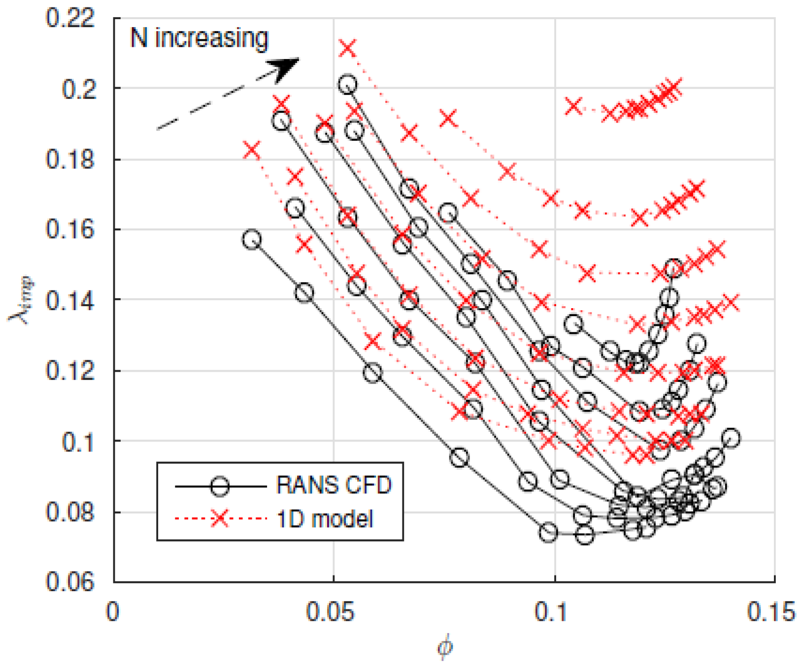
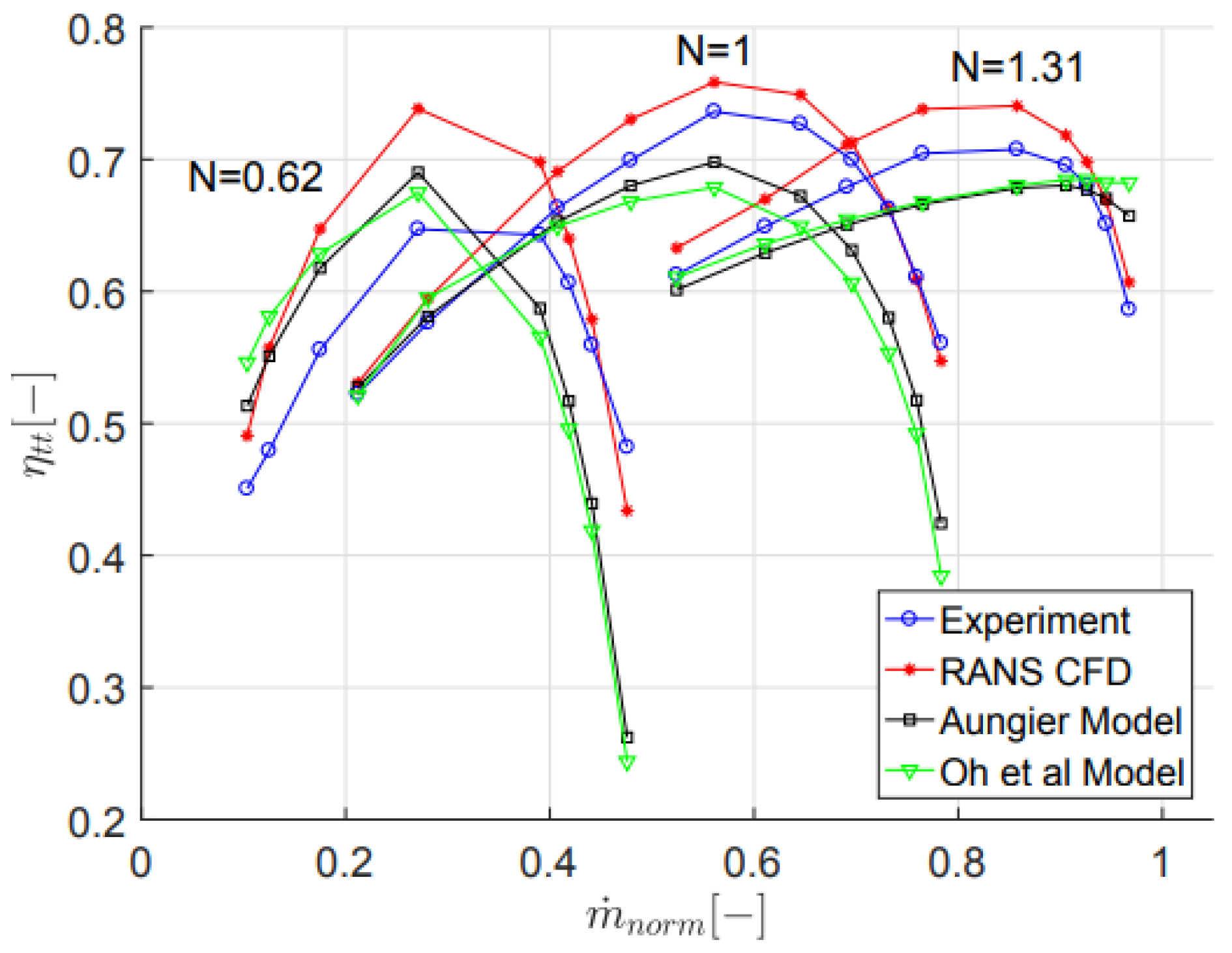
Moreover, an assessment of high-performance radial compressor parameters by 1D modelling and Reynolds-averaged Navier–Stokes (RANS) 3D computational fluid dynamics (CFD) simulation was done by Sundström et al. [22]. A loss model and a steady state RANS model by Aungier [23] were chosen for the 1D modelling and computational fluid dynamics (CFD) calculations, respectively. In addition, the centrifugal compressor examined was for automotive turbochargers, especially lightweight vehicles. The aim of the study was not only to quantify the variation between the predicted and the experimental data, but also to check the validation of the methodologies that were used.
Sundström et al. [22] in Figure 2 found that the 1D method generated accurate results at design conditions. However, at higher speed lines towards surge and choke, there was a significant variation in the results. Figure 2 presents these variations at higher speed lines. N indicates the design speed of the compressor. Furthermore, the results for the validation of the used methodologies indicated that the impeller external loss was considerably higher in the computational fluid dynamics (CFD) calculations towards surge, but this loss could not be captured by the 1D model (see Figure 3). Additionally, another significant difference was that the scroll loss was predicted to be larger in the 1D method. Lastly, the authors suggested that, by improving these major disparities in the 1D modelling method, it would be beneficial since the accuracy of the prediction method could be improved.
The present paper, therefore, is attempting to implement leading compressor preliminary performance zero-dimensional and pseudo one-dimensional techniques to the problem of implementation of these for turbocharger compressors, which are electrically assisted.

2. Centrifugal Compressor Design Methodology

The design target was an electric turbocharger compressor that could meet the boosting requirements of the engine at the specified engine speeds while offering a noticeable improvement in a transient response. For the analysis of the turbocharger compressor flows, a one-dimensional approach was applied since it is not only a fast and reliable prediction model for centrifugal compressor, but also requires a small number of input parameters [19]. The 1D modelling method is based on the fundamental fluid flow equations, thermodynamic equations, and empirical correlations [23]. These equations were obtained from the Euler’s turbomachinery theory and corresponding velocity diagrams, while the empirical relationships were obtained from experimental data. Additionally, in the 1D modelling approach, it was assumed that the flow conditions were uniform since the air would behave as an ideal gas [24].
In Figure 4, the schematic flow diagram of the compressor modelling procedure that was used for this analysis is shown and implemented in the MATLAB programming language. In addition, a crucial step for the modelling and analysis of the compressor was separating its individual components into four stages. Each stage includes the inlet or exit characteristics of the component. The compressor consists of the impeller, vaneless diffuser, and the scroll. Thus, stage one is the impeller inlet, while stage two is the impeller exit and the vaneless diffuser inlet. The impeller exit and the vaneless diffuser operate under the same flow conditions. Moreover, stage three is the vaneless diffuser exit and the scroll inlet where the conditions are again the same. Lastly, stage four is the scroll exit condition. In Figure 5, the cross-sectional schematic of the centrifugal compressor with the stage separation is shown.
To start the design procedure of the centrifugal compressor, the input parameters and the compressor geometry are required (see Table 1). Thus, the parameters that were given as designed constraints would be the inlet conditions (ambient static pressure and temperature), maximum rotational speed, air mass flow rate, and pressure ratio. As far as the compressor geometries were concerned (Table 2), they were obtained from the centrifugal compressor that was designed by Yang et al. [4]. Both input parameters and compressor geometries are shown below.

3. Non-Dimensional Loss Parameters

In this section, the non-dimensional loss models ω ¯ of the compressor components that were used for the purposes of the study were presented. Specifically, the loss models for each component were individually described and determined.

3.1. Impeller Loss Models

According to Aungier [23], the impeller losses can be converted and expressed as a total relative pressure loss defined as:
Δ P t r = f c ( P t r 1 P s 1 ) i ω ¯ i
where fc is a correction factor, which depends on the total relative density ρtr.
The mathematical descriptions of these two functions, according to Aungier [23] are described as:
f c = ρ t r 2 T t r 2 ρ t r 1 T t r 1
ρ t r = P t r R T t r
Since the impeller is the rotating component, it was essential to determine the total relative pressure and temperature, which are defined below [19].
P t r = P s [ 1 + ( γ 1 2 ) M r 2 ] γ γ 1
Τ t r = T s [ 1 + ( γ 1 2 ) Μ r 2 ]
where Mr is the relative Mach number, defined as:
M r = W γ R T s
To calculate the actual conditions of the impeller, the non-dimensional losses need to be subtracted from the isentropic conditions. However, the total relative temperatures in isentropic and actual flow are the same because the rothalpy is conserved. Thus, as far as the total relative pressure in the actual flow at the second stage is concerned, it can be calculated by subtracting the total relative pressure losses from the total relative pressure in the isentropic process. The equation is shown below [23].
P t r 2 = P t r 2 , i s Δ P t r
Furthermore, according to Bathie [25], the total pressure and temperature at the throat are described below.
T t h = T t 1 [ 2 N π ( C u 1 r m 1 C u t h r m t h ) 60 c p ]
P t h = P t 1 ( T t h T t 1 ) γ γ 1
Aungier [23] and Boyce [26] loss models were selected to determine the loss parameters of the impeller. The chosen models that are analyzed are presented in Table 3.
Moreover, each loss parameter was described and analyzed individually. Additionally, the loss model was described as a function of inlet, throat, isentropic exit, and boundary conditions such as the area, the radius of the impeller, the rotational speed, and the mass flow rate.

3.2. Vaneless Diffuser Loss Models

According to Aungier [23], the non-dimensional vaneless diffuser losses can be converted and expressed as a total pressure loss defined below.
Δ P t 3 = ( P t 2 P s 2 ) i ω ¯ i
The vaneless diffuser loss model process is similar to that in the impeller. However, the vaneless diffuser is a stationary component and the rothalpy is decreased to a constant enthalpy. Hence, the total temperature in the vaneless diffuser and the scroll is constant.
The actual conditions of the vaneless diffuser were calculated by subtracting the total pressure loss from the isentropic total pressure. The equation is shown below [23].
P t 3 = P t 3 , i s Δ P t 3
Furthermore, two loss parameters were selected to model the losses for the vaneless diffuser, the skin friction, and diffusion (Table 4) [23].

3.3. Scroll Loss Models

According to Aungier [23], the non-dimensional scroll losses can be converted and expressed as a total pressure loss, which is defined below.
Δ P t 4 = ( P t 3 P s 3 ) i ω ¯ i
As stated in the previous vaneless diffuser section, the scroll is in a stationary form. Hence, the total temperature in the scroll is constant. Furthermore, to calculate the actual pressure conditions of the scroll, the non-dimensional pressure losses need to be subtracted from the isentropic conditions. The equation is shown below [23].
P t 4 = P t 4 , i s Δ P t 4
Moreover, it has been stated that there are four non-dimensional scroll losses (Table 5) [23].

4. Modeling the Engine

For the aim of this study, two models of an engine were designed in GT-Power. The first model was sourced from an available model of the Ford Ecoboost 1.5 L, known as an inline 3-cylinder engine, which served as the baseline model with the correct turbocharger map implemented in the model. The second model had the same engine, but with the EAT implemented. The second model is shown in Figure 6.
In the above model, the motor/generator object, which represents the electrical machine of the electrically assisted turbocharger, is attached to the turboshaft.

4.1. Motor/Generator Specifications

The motor/generator parameters used for the simulation were based on an electrical machine developed by Lee and Ehsani [27]. Table 6 below shows the Brushless DC motor/generator specifications while Figure 7 illustrates the peak power and torque curves of the engine modelled.
Furthermore, the applied voltage of the battery that was used in the engine model was 48 V. The development of the electric turbocharger was initially based on (and limited by) the 12 V architecture of automobiles. However, some automobile makers have been considering the use of 48 V architectures to enhance the goal of improving the transient response for a considerable time in order to accommodate mild-hybridization requirements. According to a simulation that was conducted by Nishiwaki et al. [28] for a 48 V battery system and compared against an equivalent 12 V architecture, the simulation has shown a significant improvement in the transient response at low engine speeds (0.4 s to reach a target 1.65 pressure ratio against 1.0 s for the 12 V system).
Lastly, for the analysis presented here, it is worth noting that the thermal behavior of the motor/generator was ignored.

4.2. Engine Specifications

For the simulation of the modeled engine, it was required to import the Ford Ecoboost 1.5 L specifications for modeling the engine objects. The specifications are described in Table 7, below.

4.3. Description of the Simulation

Five cases were used for the simulation of the baseline model and electrically assisted turbocharged model. Each case had different engine speed, which varied from 1000 to 5000 rpm. Moreover, as initial conditions were given, the ambient pressure and temperature were 1.01325 bar and 298 K, respectively.
The model of the electrically assisted turbocharger was modified and analyzed for five different power levels, which varied from 1 kW to 5 kW. This is performed to study and examine how the power consumed or generated from or by the electrical machine affects the engine torque at low and high engine speed rates. The operating point used for the simulations are presented in Table 8.

5. Results and Discussion

5.1. Compressor Efficiency

The operation of the centrifugal compressor for the baseline and EAT models at low engine speed rates of 1000 rpm and 2000 rpm are presented in the following figures—the outcome of the engine simulation setup described in Section 5.
Figure 8 shows that the operation of the compressor at 1000 rpm engine speed is moved significantly to the right side of the performance map with the assistance of the motor/generator. Thus, the compressor operation has moved to a more efficient region. Moderate improvement can be observed to the operation for the 1 kW and 2 kW EAT model when compared to the baseline model. On the other hand, from 3 kW to 5 kW power models, the compressor operation has increased greatly when compared to the baseline model.
Furthermore, an important drawback is that the EAT forces the operation of the compressor to exceed the surge line of the efficiency map, which is shown in Figure 9. Therefore, map enhancement techniques should be applied to the compressor, such as casing treatment, to overcome this drawback.
As far as the 2000 rpm engine speed is concerned, the Figure illustrates that the application of the motor/generator to the turbocharger shaft pushes the operation of the centrifugal compressor toward the right side of the map. Thus, the compressor operates to a more efficient area. In addition, the Figure shows that the electrically-assisted turbocharger (EAT) models, except from the 1kW model, have significantly increased the pressure ratio of the compressor, which results in further improvement of the engine performance.

5.2. Transient Response

As can be seen from Figure 10, the transient response time of the baseline engine at 1000 rpm has been reduced by 85.6% with the electrical assistance of 5 kW (for accelerations up to 110,000 rpm out of a maximum turbocharger speed of 120,000 rpm). Moreover, the 3 kW and the 4 kW models have almost the same transient response time as the 5 kW. On the other hand, the transient response time for 2 kW configuration has been decreased by 64% when compared to the baseline model. It is worth mentioning that the application of the electrical assisted turbocharger with 1 kW was reduced only by 20% of the response time for the engine compared to the conventional turbocharger. Therefore, it is essential to install at least a 2 kW EAT to improve the performance of the engine considerably.
The results in Figure 10 indicate that the electrical assisted turbocharger of 1 kW at 1000 rpm of engine speed can decrease the transient response time of the engine by 78.4% whereas, with higher power modifications, the response time can be reduced up to 83.2%. Moreover, the fluctuations that are displayed on the graphs in Figure 11 were a result of the mass flow rate variation due to the throttle valve opening. In addition, as can be seen from Figure 11, there is an insignificant effect on the reduction of the response time among the 3 kW and the higher power level models.
Furthermore, the results from Figure 12 indicate that, as the power levels rise, not only is the response time of the engine decreased, but the BMEP is also increased significantly.
In Figure 13, the average turbocharger shaft speed over time is illustrated. Overall, the shaft speed is rapidly increased with the electrical assistance. The maximum shaft speed that was achieved by the 5 kW model peaked at 110k rpm, while the maximum speed for the models from 2 kW to 4 kW was at 105k rpm. Although the shaft speed of the 1 kW configuration increased faster than the conventional turbocharger, the maximum speed that was achieved was lower than that of the baseline model. Thus, the 1 kW model is not a preferable turbocharger for the engine.

5.3. Brake Torque and BSFC Graphs

In this section, the brake torque and the brake-specific fuel consumption of the GT-Power models over the engine speed graphs are presented and discussed. The results in Figure 14 indicate that the engine torque was significantly improved with the electrically assisted turbocharger. Especially, the highest value of torque achieved by the 5 kW model was at 240 Nm at 3000 rpm engine speed. Moreover, the torque graphs of the 3 kW and 4 kW model were almost the same, but, nonetheless, the difference can be spotted in the netBSFC map in the Figure (after power required to run the motor was subtracted). The BSFC of the 4 kW power level is slightly reduced for the engine speed range from 3000 to 4000 rpm when compared to the 3 kW EAT model.
Furthermore, as far as the 1 kW and 2 kW cases are concerned, the engine torque has been increased for both models for the engine range between 1000 to 2000 rpm and 1000 to 3000 rpm, respectively. It is worth noting that at 4000 to 5000 rpm, the torque of the EAT models has been decreased and have slight differences with the engine torque of the baseline model, which can been seen in Figure 14. This occurs because the electrically-assisted turbocharger extracts torque from the shaft at high engine speed to charge the battery of the electric machine.
The results in the Figure 15 depict the BSFC of GT-Power models. It is evident that, when the EAT is applied, the BSFC of the engine is significantly improved. Specifically, for the 5 kW model, the BSFC has been reduced by an average of 1.4% when compared to the baseline model. In addition, the 1kW has considerably decreased the BSFC for 1000 to 4000 rpm speed range whereas the BSFC has been further reduced with the electrical assistance of 2 kW. Lastly, at high engine speed, there is a slight fall in the BSFC graphs of the electrically-assisted turbocharger (EAT) models and the baseline model despite the fact that additional torque is extracted from the engine.

6. Results from the Optimized Compressor

In this section, the results obtained from GT-Power simulation for the optimized compressor, which was found by using the Matlab code are presented and discussed. Table 9 includes the optimized geometries of the centrifugal compressor, which were obtained from the MatLab code.
These geometries were applied to the GT-Power models to evaluate the effect of the optimized compressor to the engine performance. In addition, to identify the differences between the initial and the optimized compressor, a one-by-one comparison of the models was conducted.

6.1. Comparison of the Baseline Models

The results in Figure 16 shows that, overall, there was a slight increase in the engine torque with the optimized compressor. However, at high engine speed and especially from 4000 to 5000 rpm, the engine torque rose moderately. Similarly, in Figure 17, the BSFC for the optimized compressor has been slightly improved compared with the BSFC of the initial compressor.
Moreover, there was no reduction to the transient response time of the engine with the optimized compressor. However, the turbocharger shaft speed for 1000 rpm engine speed has peaked to a higher value than the initial compressor design, as is shown in Figure 18.

6.2. Comparison of the EAT with 1 kW Power Level Models

The results obtained from the simulations for the initial and optimized compressor of the electrical assisted turbocharger models with power level 1 kW indicate that there is no significant difference between the two compressors. Figure 19 shows the engine torque versus engine speed for both centrifugal compressors. Even though the two graphs are very similar, there is a slight rise of the torque for the optimized compressor at an engine speed range between 4000 to 5000 rpm.
Similarly, as can been seen from Figure 20, the BSFC for both compressors are almost the same except for the engine speed range of 1000–2000 rpm in which the BSFC of the optimized compressor has been slightly increased. However, the results indicated that, with the optimized compressor, there is an insignificant improvement in the engine performance.

6.3. Comparison of the EAT with 2 kW Power Level Models

The optimized compressor in the EAT model with 2 kW power level configuration has significantly improved the overall performance of the engine. Especially, as shown in Figure 21, from 2000 to 4000 rpm, the engine torque of the optimized compressor has increased moderately compared to the initial design of the compressor. On the other hand, at low engine speed, the brake torque for both compressors was the same while, at high engine speed, the initial compressor had greater engine torque than the optimized compressor.
The graphs in Figure 22 present the BSFC over the engine speed for the initial and the optimized compressor. It is evident that, at the engine speed range of 2000–4000 rpm, the brake specific fuel consumption (BSFC) has been considerably reduced with the optimized compressor while, at high engine speed, the brake specific fuel consumption (BSFC) is slightly increased when compared to the initial compressor. Moreover, the results in Figure 23 indicate that the transient response time of the engine model with the optimized compressor was reduced by 25%.

6.4. Comparison of the EAT with 3 kW and 4 kW Power Level Models

The results obtained from the GT-Power simulations show that, in the electrically-assisted turbocharger (EAT) models of 3 kW despite the change on the compressor, the engine performance remained steady. Similarly, it has been found that the electrically-assisted turbocharger (EAT) model of 4 kW with the optimized compressor has the same results with the initial compressor model. In the following Figure 24, Figure 25, Figure 26 and Figure 27, results of the 3 kW as well the 4 kW models are presented for brake torque (Figure 24 and Figure 25) and brake mean effective pressure (BMEP; Figure 26 and Figure 27).
As can be seen from the above figures, the results of the baseline and optimized compressor totally match for both modelling cases 3 kW and 4 kW. One plausible reason for the results that occurred could be an error in the simulations for these cases. Moreover, another explanation could be that, in the optimized compressor, the exit diameter of the impeller was slightly reduced. Therefore, the change did not significantly affect the performance of the engine, as in the electrically assisted turbocharger (EAT) 1 kW case.

6.5. Comparison of the EAT with 5 kW Power Level Models

In this section, a comparison between the engine model with the optimized compressor and the engine model with the initial compressor was conducted. Figure 28 presents the brake torque of the two models versus engine speed. It is clear that the engine torque has considerably risen with the optimized centrifugal compressor in place. Especially from 1000 rpm, the engine torque is increased gradually until 3000 rpm where the engine torque peaks at 293.2 N. However, from 4000 to 5000 rpm, the torque is decreased sharply and matches with the values of the torque of the engine model with the initial compressor.
In addition, the results in Figure 29 indicate that, overall, the brake-specific fuel consumption (BSFC) of the engine model with the optimized compressor has been considerably reduced when compared with the engine model with the initial compressor. Furthermore, the highest reduction in the brake-specific fuel consumption BSFC of the electrically-assisted turbocharger (EAT) model occurred at low engine speed.
Moreover, Figure 30 outlines the average turbocharger shaft speed for the two engine models against time. Although the transient response time remained steady with the optimized compressor model, the maximum shaft speed has increased by 3000 rpm, as shown in Figure 28. Therefore, the overall performance of the engine model with the optimized compressor has improved.

7. Conclusions

A design methodology is implemented based on authoritative loss models for the preliminary design of a centrifugal electrically-assisted turbocharger (EAT) compressor. The methodology was extended to engine performance modeling for a conventionally and an electrically-assisted turbocharger (EAT)-equipped engine layout. The calculated compressor geometry arising from the proposed method was imported to the engine simulation software while the EAT-equipped engine was tested at five different power levels from 1 kW to 5 kW.
The results obtained from the engine simulations indicated that the electrically-assisted turbocharger (EAT) engine model improved the overall performance of the engine compared to the baseline engine. Moreover, the electrically-assisted turbocharger (EAT) equipped engine power output with 1 kW and 5 kW electrically-assisted turbocharger (EAT) power levels was increased by an average of 5.96% and 15.4%, respectively, from 1000 to 3000 rpm engine speed when compared to the baseline model.
As far as the BSFC is concerned for the electrically-assisted turbocharger (EAT) model for 1 kW and 5 kW, there was an overall fuel consumption decrease of 0.53% and 1.45% depending on engine operating conditions, respectively, when compared to the initial baseline engine model.

Author Contributions

N.X. and M.A. were the research students that conducted the detailed study and wrote the first draft of this paper. A.P. conceived of the project, created the layout of the investigations, and checked the computational outcome of the resultant modelling effort and subsequent discussion.

Funding

This research received no external funding.

Conflicts of Interest

The authors declare no conflict of interest.

Nomenclature

Variables
CmMeridional component of absolute velocity [m/s]
CuTangential component of absolute velocity [m/s]
CpSpecific heat at constant pressure [J/(kg·K)]
NRotational speed of turbocharger [rpm]
PPressure [bar]
RGas constant for air [J/(kg·K)]
rRadius [mm]
TTemperature [K]
Subscripts
0Stagnation or total state; ambient condition
1-4compressor stages
is, sisentropic
mMeridional velocity component
rRadial velocity component
rmsRoot mean square
ThThroat parameter
TrTotal relative
Greek letters
γRatio of specific heats
ΔDifference
ρDensity [kg/m3]
ω Non-dimensional pressure loss
Acronyms
BMEPBrake mean effective pressure
BSFCBrake-specific fuel consumption
EATElectrically assisted turbocharger
MGMotor-Generator
RANSReynolds Averaged Navier Stokes
rpmRevolution per minute

References

  1. Winterbone, D.E.; Benson, R.S.; Mortimer, A.G.; Kenyon, P.; Stotter, A. Transient Response of Turbocharged Diesel Engines. In Proceedings of the 1977 International Automotive Engineering Congress and Exposition, Detroit, MI, USA, 28 February–4 March 1977. [Google Scholar] [CrossRef]
  2. Pesiridis, A.; Ferrara, A.; Tuccillo, R.; Chen, H. Conceptual design of an axial turbocharger turbine. In Proceedings of the ASME Turbo Expo 2017: Turbomachinery Technical Conference and Exposition, Charlotte, NC, USA, 26–30 June 2017; Volume 8, pp. 1–12. [Google Scholar] [CrossRef]
  3. Pesiridis, A.; Saccomanno, A.; Tuccillo, R.; Capobianco, A. Conceptual Design of a Variable Geometry, Axial Flow Turbocharger Turbine. SAE Tech. Pap. 2017. [Google Scholar] [CrossRef]
  4. Yang, M.Y.; Martinez-Botas, R.F.; Zhuge, W.L.; Qureshi, U.; Richards, B. Centrifugal compressor design for electrically assisted boost. In IOP Conference Series: Materials Science and Engineering; IOP Publishing: Bristol, UK, 2013; Volume 52, p. 042014. [Google Scholar] [CrossRef]
  5. Grönman, A.; Sallinen, P.; Honkatukia, J.; Backman, J.; Uusitalo, A. Design and experiments of two-stage intercooled electrically assisted turbocharger. Energy Convers. Manag. 2016, 111, 115–124. [Google Scholar] [CrossRef]
  6. Terdich, N.; Martinez-Botas, R.F.; Romagnoli, A.; Pesiridis, A. Mild Hybridization Via Electrification of the Air System: Electrically Assisted and Variable Geometry Turbocharging Impact on an Off-Road Diesel Engine. J. Eng. Gas Turbines Power 2013, 136, 31703. [Google Scholar] [CrossRef]
  7. Harley, P.; Spence, S.; Filsinger, D.; Dietrich, M.; Early, J. Experimental and Numerical Benchmarking of an Improved Meanline Modelling Method for Automotive Turbocharger Centrifugal Compressors. In Proceedings of the ASME Turbo Expo 2015: Turbine Technical Conference and Exposition, Montreal, QC, Canada, 15–19 June 2015; Paper No. GT2015-42175. p. V02CT42A008. [Google Scholar]
  8. Feneley, A.; Pesiridis, A.; Chen, H. A One-Dimensional gas dynamics code for turbocharger pulsating flow and heat transfer performance modelling. In Proceedings of the ASME TURBO EXPO 2017 (ASME GT2017-64743), Charlotte, NC, USA, 26–30 June 2017. [Google Scholar]
  9. Rodgers, C.; Sapiro, L. Design Considerations for High-Pressure-Ratio Centrifugal Compressors. In Proceedings of the ASME 1972 International Gas Turbine and Fluids Engineering Conference and Products Show, San Francisco, CA, USA, 26–30 March 1972; (Paper No. 72-GT-91). p. V001T01A090. [Google Scholar]
  10. Rajoo, S.; Romagnoli, A.; Martinez-Botas, R.; Pesiridis, A.; Copeland, C.; Mamat, A.M.I. Automotive Exhaust Waste Heat Recovery Technologies. In Automotive Exhaust Emissions and Energy Recovery; NOVA Science Publishers: Hauppage, NY, USA, 2014; ISBN 978-1-63321-493-4. [Google Scholar]
  11. Katrašnik, T.; Rodman, S.; Trenc, F.; Hribernik, A.; Medica, V. Improvement of the Dynamic Characteristic of an Automotive Engine by a Turbocharger Assisted by an Electric Motor. J. Eng. Gas Turbines Power 2003, 125, 590. [Google Scholar] [CrossRef]
  12. Baines, N.C. Fundamentals of Turbocharging; Concepts NREC: White River Junction, VT, USA, 2005. [Google Scholar]
  13. Harley, P.; Spence, S.; Filsinger, D.; Dietrich, M.; Early, J. Meanline Modeling of Inlet Recirculation in Automotive Turbocharger Centrifugal Compressors. J. Turbomach. 2014, 137, 011007. [Google Scholar] [CrossRef]
  14. Galvas, M.R. Fortran Program for Predicting Off-Design Performance of Centrifugal Compressors; Report NASA-TN-D-7487, E-7480; National Aeronautics and Space Administration: Washington, DC, USA, 1973.
  15. Serrano, J.R.; Arnau, F.J.; García-Cuevas, L.M.; Dombrovsky, A.; Tartoussi, H. Development and validation of a radial turbine efficiency and mass flow model at design and off-design conditions. Energy Convers. Manag. 2016, 128, 281–293. [Google Scholar] [CrossRef]
  16. Feneley, A.J.; Pesiridis, A.; Andwari, A.M. Variable Geometry Turbocharger Technologies for Exhaust Energy Recovery and Boosting—A Review. Renew. Sustain. Energy Rev. 2017, 71, 959–975. [Google Scholar] [CrossRef]
  17. Shah, S.V.; Vyas, B.G.; Bollavarapu, A.; Patel, S. Aerodynamic and Thermal Design of Centrifugal Compressor for Small Scale in Non-Dimemsional Form. Int. J. Mech. Prod. Eng. Res. Dev. 2017, 7, 81–92. [Google Scholar]
  18. Johnston, J.P.; Dean, R.C.J. Losses in Vaneless Diffusers of Centrifugal Compressors and Pumps: Analysis, Experiment, and Design. J. Eng. Power 1966, 88, 49–60. [Google Scholar] [CrossRef]
  19. Kerres, B.; Sanz, S.; Sundström, E.; Mihaescu, M. A Comparison of Performance Predictions between 1D Models and Numerical Data for a Turbocharger Compressor. In Proceedings of the 12th European Conference on Turbomachinery Fluid dynamics & Thermodynamics, Stock, Sweden, 3–7 April 2017. [Google Scholar]
  20. Aungier, R.H. Mean Streamline Aerodynamic Performance Analysis of Centrifugal Compressors. J. Turbomach. 1995, 117, 360–366. [Google Scholar] [CrossRef]
  21. Oh, H.W.; Yoon, E.S.; Chung, M.K. An optimum set of loss models for performance prediction of centrifugal compressors. Proc. Inst. Mech. Eng. Part A J. Power Energy 1997, 211, 331–338. [Google Scholar] [CrossRef]
  22. Sundström, E.; Kerres, B.; Sanz, S.; Mihăescu, M. On the Assessment of Centrifugal Compressor Performance Parameters by Theoretical and Computational Models. In Proceedings of the ASME Turbo Expo 2017: Turbomachinery Technical Conference and Exposition, Charlotte, NC, USA, 26–30 June 2017. [Google Scholar]
  23. Aungier, R.H. Centrifugal Compressors: A Strategy for Aerodynamic Design and Analysis; ASME Press: New York, NY, USA, 2000. [Google Scholar]
  24. Japikse, D.; Baines, N.C. Introduction to Turbomachinery; Concepts ETI: Norwich, VT, USA, 1994. [Google Scholar]
  25. Bathie, W.W. Fundamentals of Gas Turbines; Wiley: New York, NY, USA, 1984. [Google Scholar]
  26. Boyce, M.P. Centrifugal Compressors: A Basic Guide; Pennwell Books: Tulsa, OK, USA, 2003. [Google Scholar]
  27. Lee, B.K.; Ehsani, M. Advanced Simulation Model for Brushless DC Motor Drives. J. Electr. Power Compon. Syst. 2003, 31, 841–868. [Google Scholar] [CrossRef]
  28. Nishiwaki, K.; Iezawa, M.; Tanaka, H.; Goto, T.; An, B. Development of High Speed Motor and Inverter for Electric Supercharger. SAE Tech. Pap. 2013. [Google Scholar] [CrossRef]
  29. Ford Media. Available online: https://media.ford.com/content/dam/fordmedia/Europe/documents/productReleases/Focus/FordFocus_TechSpecs_EU.pdf (accessed on 1 January 2018).
Figure 1. Isentropic Efficiency of the Experiment compared with Reynolds-averaged Navier–Stokes (RANS) computational fluid dynamics (CFD), and the two prediction models.
Energies 12 00975 g001
Figure 2. Comparison on the isentropic efficiency in the experiment including the Reynolds-averaged Navier–Stokes (RANS) computational fluid dynamics (CFD) and 1D model.
Energies 12 00975 g002
Figure 3. Impeller Losses of RANS CFD and the 1D Model.
Energies 12 00975 g003
Figure 4. Compressor modelling procedure flow diagram.
Energies 12 00975 g004
Figure 5. Centrifugal Compressor cross-section schematic labelling the stages.
Energies 12 00975 g005
Figure 6. Model of the Ford Ecoboost 1.5L electrically assisted turbocharged engine.
Energies 12 00975 g006
Figure 7. Performance of the based turbo-charged engine.
Energies 12 00975 g007
Figure 8. Compressor performance at 1000 rpm engine speed with efficiency contours.
Energies 12 00975 g008
Figure 9. Compressor performance at 2000 rpm engine speed.
Energies 12 00975 g009
Figure 10. Turbocharger shaft speed at a 1000 rpm engine.
Energies 12 00975 g010
Figure 11. Brake Mean Effective Pressure (BMEP) response time at 1000 rpm engine speed.
Energies 12 00975 g011
Figure 12. Brake mean effective pressure response time at 2000 rpm engine speed.
Energies 12 00975 g012
Figure 13. Turbocharger shaft speed at the 2000 rpm engine speed.
Energies 12 00975 g013
Figure 14. Engine torque results from the engine model.
Energies 12 00975 g014
Figure 15. BSFC map results from the engine model.
Energies 12 00975 g015
Figure 16. Brake torque versus engine speed for the initial and the optimized baseline models.
Energies 12 00975 g016
Figure 17. BSFC graphs for the initial and optimized baseline models.
Energies 12 00975 g017
Figure 18. Average Shaft speed of the baseline models at 1000 rpm engine speed.
Energies 12 00975 g018
Figure 19. Brake torque over engine speed for the initial and the optimized EAT 1 kW models.
Energies 12 00975 g019
Figure 20. BSFC graphs for the initial and optimized EAT 1 kW models.
Energies 12 00975 g020
Figure 21. Brake Torque graphs for the initial (black) and optimized (green) EAT 2 kW models.
Energies 12 00975 g021
Figure 22. BSFC graphs for the initial and optimized EAT 2kW models.
Energies 12 00975 g022
Figure 23. Average Shaft speed of the electrically-assisted turbocharger (EAT) models with 2 kW power level at 1000 rpm engine speed.
Energies 12 00975 g023
Figure 24. Brake torque of the electrically-assisted turbocharger (EAT) 3 kW model for the initial and optimized compressor.
Energies 12 00975 g024
Figure 25. Brake torque of the electrically-assisted turbocharger (EAT) 4 kW model for the initial and optimized compressor.
Energies 12 00975 g025
Figure 26. Brake mean effective pump (BMEP) graphs of the EAT 3 kW model for the initial and optimized compressor.
Energies 12 00975 g026
Figure 27. Brake mean effective pressure (BMEP) graphs of the EAT 4 kW model for the initial and optimized compressor.
Energies 12 00975 g027
Figure 28. Brake torque graphs for the initial (black) and optimized (green) EAT 5 kW models.
Energies 12 00975 g028
Figure 29. Brake-specific fuel consumption (BSFC) graphs for the initial and optimized electrically assisted turbocharger (EAT) 5 kW models.
Energies 12 00975 g029
Figure 30. Average shaft speed of the electrically assisted turbocharger (EAT) models with 5 kW power level at 1000 rpm engine speed.
Energies 12 00975 g030
Table 1. Operating conditions for the centrifugal compressor.
Input ParametersMetric Units
Ambient Static Pressure1.01325 bar
Ambient Static Temperature298 K
Maximum Rotational Speed120,000 rpm
Air Mass Flow Rate0.08 kg/s
Table 2. Main compressor geometry [4].
Geometrical ParametersValues
Inlet hub radius R1h6.2 mm
Inlet shroud radius R1s17.2 mm
Impeller exit radius R229.1 mm
Exit blade height b23.4 mm
Blade number Z5 + 5
Blade angle at inlet tip β1b-shroud−62 deg
Diffuser exit radius R340.75 mm
Scroll throat area Ath397 mm2
Table 3. Impeller loss models used for the study [23,26].
Impeller Loss Models
1. Shock2. Incidence
3. Diffusion4. Choke
5. Skin friction6. Clearance gap
7. Blade loading8. Hub-shroud loading
9. Wake mixing10. Expansion
11. Supercritical Mach number
Table 4. Vaneless diffuser loss models.
Vaneless Diffuser Loss Models
1. Skin friction2. Diffusion
Table 5. Scroll loss models.
Scroll Loss Models
1. Meridional velocity loss2. Tangential velocity loss
3. Skin friction4. Exit cone loss
Table 6. Motor/generator specifications.
AttributeObject ValueUnits
Torque Constant0.0042Nm/A
Equivalent Resistance3Ohm
Equivalent Inductance1.22mH
Friction Torque0.662Nm
Stall Current200A
Inertia8.2614 × 10−5Kg/m2
Table 7. Ford Focus, Ecoboost 1.5 L, 3-cylinder petrol engine specification [29].
AttributeObject ValueUnit
Bore 83Mm
Stroke92.4Mm
Connecting Rod Length137Mm
Compression Ratio10.4----
TDC Clearance Height1mm
Max.Brake Power 110kW
Max. Brake Torque240Nm
Min. Brake Specific Fuel Consumption (@3000 rpm)234g/kWh
Valves4
Table 8. The operating points that were used for the simulation.
Operating PointTurbochargerMaximum Power
Baseline Conventional-
Operating Point 1EAT1 kW
Operating Point 2EAT2 kW
Operating Point 3EAT3 kW
Operating Point 4EAT4 kW
Operating Point 5EAT5 kW
Table 9. Optimization results for B = 0.02 and N = 120,000 rpm.
r1h [m]0.001Zr [-]10
r1t [m]0.0113βB2 [°]−45
M1t [-]0.7015DR [-]1.6682
β1 [°]15.1548Nstage [-]0.4361
Af1 [m2]3.9555 × 10⁴b2 [m]0.0047
U1t [m/s]141.5642r2 [m]0.0294
W1t [m/s]231.0347U2 [m/s]369.6808
Cm1 [m/s]223W2 [m/s]138.4913
Cu1 [m/s]81.1653M2 [-]0.6807
C1 [m/s]237.3116

