Guidelines and Cost-Benefit Analysis of the Structural Health Monitoring Implementation in Offshore Wind Turbine Support Structures

Abstract

This paper investigates how the implementation of Structural Health Monitoring Systems (SHMS) in the support structure (SS) of offshore wind turbines (OWT) affects capital expenditure (CAPEX) and operational expenditure (OPEX) of offshore wind farms (WF). In order to determine the added value of Structural Health Monitoring (SHM), the balance between the reduction in OPEX and the increase in CAPEX is evaluated. In this paper, guidelines for SHM implementation in offshore WF are developed and applied to a baseline scenario. The application of these guidelines consist of a review of present regulations in the United Kingdom and Germany, the development of SHM strategy, where the first stage of the Statistical Pattern Recognition (SPR) paradigm is explored, failure modes that can be monitored are identified, and SHM technologies and sensor distributions within the turbines are described for a baseline scenario. Furthermore, an inspection strategy where the different structural inspections to be carried out above and below water is also developed, together with an inspection plan for the lifetime of the structures, for the aforementioned baseline scenario. Once the guidelines have been followed and the SHM and inspection strategies developed, a cost-benefit analysis is performed on the baseline case (10% instrumented assets) and three other scenarios with 20%, 30% and 50% of instrumented assets. Finally, a sensitivity analysis is conducted to evaluate the effects of SHM hardware cost and the time spent in completing the inspections on OPEX and CAPEX of the WF. The results show that SHM hardware cost increases CAPEX significantly, however this increase is much lower than the reduction in OPEX caused by SHM. The results also show that an increase in the percentage of instrumented assets will reduce OPEX and this reduction is considerably higher than the cost of SHM implementation.

1. Introduction

Over the past 15 years, wind energy has experienced a remarkable growth in Europe. This is partially due to the long-term goal set by the European Commission (EC) to lower greenhouse gas emissions by 80–95% by 2050, compared to levels in the 1990’s. This target has had significant implications for renewable energy development, which has experienced a rapid growth in the past few years. Wind power technologies (including onshore and offshore) play a crucial role in reaching Europe’s renewable energy targets. The offshore wind industry in Europe is moving fast to being a mainstream supplier of low-carbon electricity [1]. In 2017 alone, about 3150 MW new offshore wind power capacity was connected to the grid. This is twice more than in 2016 and 13% higher than in 2015, which was until now the record year for offshore wind power installation [2]. This rapid development is not only due to the targets set by the EC in 2006 for all Member States [3], but also due to the scalability of wind energy with units of larger capacity been deployed in larger farms, further offshore [4].

The United Kingdom (U.K.) currently has 36 large wind farms (WF), generating 20.8 TWh of electricity, which supplies on average 6.2% of the nation’s electricity demand [5]. Furthermore, by the end of 2017, 2923 turbines were either operational or under construction, reaching a cumulative installed capacity of 5.83 GW, which will soon reach 10.4 GW once turbines being commissioned are energised [5]. Moreover, in February 2018 the 7 GW milestone was reached, which highlights the industry’s progression. With all this growth taking place, areas close to shore and with good wind resource are running out and WF tend to be developed further from shore, which usually implies deeper waters. As was reported by WindEurope [2], the average water depth of offshore wind farms (OWF) with grid connections in 2017 was 27.5 m, whereas the average distance to shore was 41 km.

A key factor in the rapid development of the offshore wind industry is the substantial reduction in the Levelised Cost of Energy (LCoE) experienced in the past few years, which enhanced and stimulated investors’ interest in the industry. In 2013, the LCoE for offshore wind energy was €140/MWh [6], but over the last few years this has cost plummeted, surpassing the 2020 target of €100/MWh. Vattenfall’s offshore wind price bid of €49.9/MWh in 2016 for the Kriegers Flak project set a record LCoE forecast of €40/MWh [7]. In order to achieve and maintain the expected cost reductions and ensure the cost-competitiveness of offshore wind in the energy sector, offshore wind operators are currently investigating ways to optimise CAPEX and OPEX, which will lead to an LCoE reduction. An alternative route to reduce OPEX, and subsequently LCoE, is through the optimisation of the inspection and maintenance strategies. This optimisation is carried out by switching periodic or risk-based inspection regimes to a condition-based regime. In order to do so, periodic inspections can be postponed or directly taken out of the scope of works whenever the condition of the assets is proven to be appropriate. SHMS are currently the best approach to gain confidence in the assets’ integrity without actually deploying offshore. Furthermore, depending on the country, regulations about inspection regimes and monitoring of offshore assets may differ.

Today, a few technical guidelines for SHM exist and these are mainly focused on civil infrastructure, such as bridges [8]. These were developed and published by national or international scientific or technical organizations [9,10,11,12,13]. In the offshore wind field, Germanischer Lloyd—one of the leading certification organizations—published a guideline for the certification of condition monitoring systems for wind turbines [14]. This guideline focusses mainly on the rotating parts of an OWT (CMS), but also includes requirements for SHM of the SS. Nevertheless, guidelines for SHM implementation in a holistic way constitute a research gap in the academic literature. For the sake of clarity, a distinction needs to be made between “guidelines for the implementation of SHM technologies” and “guidelines for SHM implementation”. The former refers to the process of determining how a particular technology would be applied into a given turbine. It will involve different aspects, such as the number of sensors, where these sensors will be located, their distribution, redundancies, number of channels for the data acquisition unit, the data transmission system and data storage, among others. The latter refers to the integration of different SHM technologies to optimise the structural integrity of an asset holistically and the understanding of the environmental and geographic challenges, design weaknesses and the expected failure mechanisms associated with this asset. It involves the development of a SHM strategy that increases confidence in the structural integrity of the assets as a whole, complying with local legislation and aiming for an economic benefit.

This paper aims to deliver guidelines for the correct SHM implementation to the SS of a baseline OWF. An increase in implementation of these systems will enhance operators’ confidence in the structural integrity of OWT SS and reduce the number of inspections they need during their lifetime. An example of the application of these guidelines is also provided for the baseline scenario, which is employed later in Section 3. An economic analysis is performed for the baseline WF to evaluate the benefits of SHM implementation in terms of reduction in OPEX, based on the previously developed guidelines. Furthermore, a comparison is made between the achieved OPEX reduction and the incurred cost of SHM implementation. The organisation of this paper is as follows. Section 2 presents the guidelines for SHM implementation, which when installed from the beginning of the operation on the WF, could be used to adopt a condition-based inspection strategy for reducing OPEX. In Section 3, a cost-benefit analysis of the impact of SHMS implementation in OPEX reduction is carried out based on the applied guidelines developed in Section 2. These results are presented and discussed in Section 4 and followed by general conclusions in Section 5.

2. Guidelines for Structural Health Monitoring Implementation in Offshore Wind Support Structures

This section presents the process to be followed for the implementation of SHMS in OWF’s SS from the design stage. The reason why SHM needs to be considered early during design is to consistently capture the loading conditions of the turbines throughout the life of the structures (not only operational life, but also during the installation-energisation and stop-of production and decommissioning) and to determine whether the structural integrity of the units is as good as expected, or if anything is compromising it. SHM not only provides confidence in the condition-based inspection and maintenance strategy but can also be used in the structural integrity evaluation process of the assets in order to obtain certification and permits from governmental authorities. If SHMS are designed, installed and their data analysed appropriately, OPEX could be reduced, even though their implementation would have a slight increase in CAPEX associated with the commissioning stage. Nevertheless, this increase in CAPEX would be justified by the higher decrease in OPEX experienced throughout the operational life of the units. The proposed guidelines for SHM implementation consist of five stages:

• To obtain a clear understanding of the legislation regulating the territory where the OWF will be developed.
• To perform an analysis of the design drivers and challenges (i.e., sand banks that make the structures prone to scour development or a high tidal range that compromises accessibility) and failure mechanisms expected for the preferred design concept.
• To develop a SHM strategy based on the failure mechanisms that can be monitored.
• To develop an inspection strategy that takes into consideration points I, II, and III and that becomes an economic justification for SHM implementation.
• To verify the economic feasibility of the proposed SHM strategy implementation. If the SHM implementation does not achieve a higher OPEX reduction than the associated CAPEX increase, either the SHM and inspection strategies should be reconsidered, or an alternative justification for the aforementioned implementation should be found (ie., an OWF is already in operation and SHMS are being implemented after there is the risk of a failure mechanism occurring).

In the following subsections, the different stages of the SHM implementation guidelines are developed and applied to a baseline. The regulations concerning the inspection and maintenance of offshore wind assets in the United Kingdom and Germany are reviewed (Section 2.1). A methodology for the development of a SHM strategy at a WF level is presented (Section 2.2), and an inspection strategy for a baseline scenario is provided (Section 2.3) for the posterior cost-benefit analysis carried out in Section 3.

2.1. Regulations and Standards

In the offshore industries, operations often take place within the limits of territorial waters and a state’s exclusive economic zone (EEZ). Legislative frameworks that are applicable to offshore wind assets depend on the coastal state in whose waters they are installed. All states regulate the activities on their EEZ, however, international law must also be observed. The United Kingdom and Germany have been chosen as examples of the two European countries with the highest installed wind power capacity in 2017 [2]. The regulations concerning inspection and maintenance of offshore wind assets in these two countries have been reviewed and compared below.

In the United Kingdom, The Department for Energy and Climate Change (DECC) [15] has overall responsibility for offshore energy projects, though some responsibilities in England and Wales are delegated to the Marine Management Organisation (MMO) and powers are devolved to the Scottish Executive for Scottish projects. The Maritime and Coastguard Agency (MCA), as an executive agency of the Department for Transport and the Health and Safety Executives of Great Britain and Northern Ireland (HSE and HSENI), hold the main responsibilities for health and safety regulations in the United Kingdom’s offshore wind industry. While floating structures are regulated by the MCA, fixed-bottom structures on the U.K. continental shelf are regulated by the HSE.

In terms of inspection requirements, there is no entity or regulatory body imposing periodic inspection intervals. It is up to the operator to take care of the integrity of its assets. However, in order to get the appropriate insurance, the assets need to be certified by a certification body (i.e., DNV GL (Det Norske Veritas Germanischer Lloyd), Lloyds Register, etc.). Technical evidence proving that the assets have been designed, inspected and maintained following best practices and regulations (when applicable) must be provided to these certification authorities by the operators.

In contrast to the United Kingdom, Germany has a more complicated process for obtaining the consent for installation and operation of OWF. The Bundesamt für Seeschifffahrt und Hydrographie (BSH) [16] is the regulating authority for offshore wind projects in German waters. All inspection and maintenance performed on the offshore wind assets (WT, substation, array cables, onshore base and port, etc.) must be done in accordance with the requirements set out in the corresponding standards in their current version, as well as current state-of-the-art requirements for certification. BSH standards are listed in

Table 1. Bundesamt für Seeschifffahrt und Hydrographie (BSH) regulations to be abided for the development and operation of offshore wind farms (OWF) in Germany.

Regulating Authority	Standard Document	Ref
BSH	Minimum requirements concerning the constructive design of offshore structures within the Exclusive Economic Zone (EEZ)	[17]
	Design of offshore wind turbines	[18]
	Minimum requirements for geotechnical surveys and investigations into offshore wind energy structures, offshore stations and power cables.	[19]
	Investigation of the impacts of offshore wind turbines (OWT) on the marine environment (StUK4)	[20]

.

One of the key requirements imposed by the BSH for the development of offshore wind projects is that the design of these projects is certified by a certification authority (e.g., DNVGL, Lloyds Register, etc.). In order to acquire this certification some technical codes of practice that shall be taken into account in the design and marine operations of the WF. These are listed in

Table 2. Technical standards for the design and operation of OWF.

Standard Document	Regulated Subject	Ref
ISO 19901-6	Petroleum and natural gas industries. Specific requirements for offshore structures, Part 6: marine operations	[21]
ISO 19905-1	Petroleum and natural gas industries. Site-specific assessment of mobile offshore units, Part 1: Jack-ups	[22]
ISO/DIS 29400	Ships and marine technology. Offshore wind energy—Port and marine operations	[23]
EN 1990	Basis of structural design	[24]
EN 1997	Eurocode 7: Geotechnical design	[25]
EN 1993	Eurocode 3: Design of steel structures	[26]
DNV-OS-H101	DNV offshore standard—marine operations, general	[27]
GL-IV-7	GL rules for the certification and construction, IV industrial services, Part 7: Offshore substations	[28]
GL-IV-6	GL rules for the certification and construction, IV industrial services, Part 6: Offshore technology	[29]
API RP-2A-WSD	American Petroleum Institute, Recommended Practice. Planning, designing and constructing fixed offshore platforms—working stress design	[30]
GL-IV-2	GL rules and guidelines, IV industrial services. Part 2: Guideline for the certification of offshore wind turbines	[31]
DNV-OS-J101	DNV offshore standard. Design of offshore wind turbine structures	[32]
DNV-OS-J201	DNV offshore standard. Offshore substations for wind farms	[33]

.

Furthermore, there are two special consent approvals to be obtained. These concern the inspection and maintenance regimes of the grouted connection (GC) in both the offshore substation and wind turbines. Maintenance of the equipment installed on the offshore assets is to be carried out with consideration of the original equipment manufacturer’s recommendations and particular warranty conditions, as well as any applicable statutory requirement related to the certification of the equipment as listed below. Nevertheless, as this paper is focused on offshore wind assets’ SS, inspection and maintenance of this equipment is considered out of scope. Aside from the standards listed above, the Periodic Inspection Concept needs to meet the outstanding conditions from the certification reports (i.e., standards listed above). These conditions are listed in

Table 3. Minimum requirements for the periodic inspection of SS according to the BSH [8].

Test Object	Test Basis and Intervals
Functionality of the anodes or impressed-current system	During the first 2 years: annually After the first 2 years: depending on the condition (recommended every 4 years)
Substructure: welded seams (subject to cyclic loads), intactness of the surface of the structural elements	In accordance to the life cycle calculations and inspection plan
Composition of the seabed surface, scouring	During the first 2 years: annually After the first 2 years: depending on the condition (recommended every 4 years)
Corrosion protection (visual inspection): Underwater area of the structure Alternating load Underwater area of the substructure Operational structure (SS)	Depending on the condition (recommended every 4 years) Depending on the condition (recommended every 2 years) Depending on the condition (recommended every 4 years) Depending on the condition (recommended every 4 years)
Operational structure: welded seams (subject to cyclic loads), bolts	In accordance to the life cycle calculations and inspection plan

:

The areas and locations to be subjected to periodical inspections are to be selected based on a risk-based prioritisation. Based on standard recommendations [34], the interval between inspections of critical items should not exceed one year. For less critical items, longer intervals are acceptable. All the structural assets should be inspected at least once every five-year period. This could be taken as one single inspection in that period, or as the inspection of a certain percent of the total number of assets on a regular basis. The latter is considered a more sensible approach, as it enables the operator to have a continuous record of the integrity of the structural assets, e.g., 20% of OWT foundations on an annual basis.

Ultimately, the risk-based SHM of the structural assets shall be used to reduce the scope of structural inspections in some cases, upon demonstration of the appropriate integrity level of the assets. These methods are meant to be employed for the entire operational life of the SS, modifying the scope of inspections and their periodicity, based on the findings and real condition of the assets. These periodic inspections shall provide evidence that the SS continues to comply with the design assumptions and that findings and observations are within the operational limits. If the periodical inspections or continuous SHM on selected locations reveal that degradation mechanisms are not developing as expected, unscheduled inspections or remedial works may be required. Unscheduled activities can be also triggered following an incident or event likely to have affected the structural integrity.

2.2. SHM Strategy

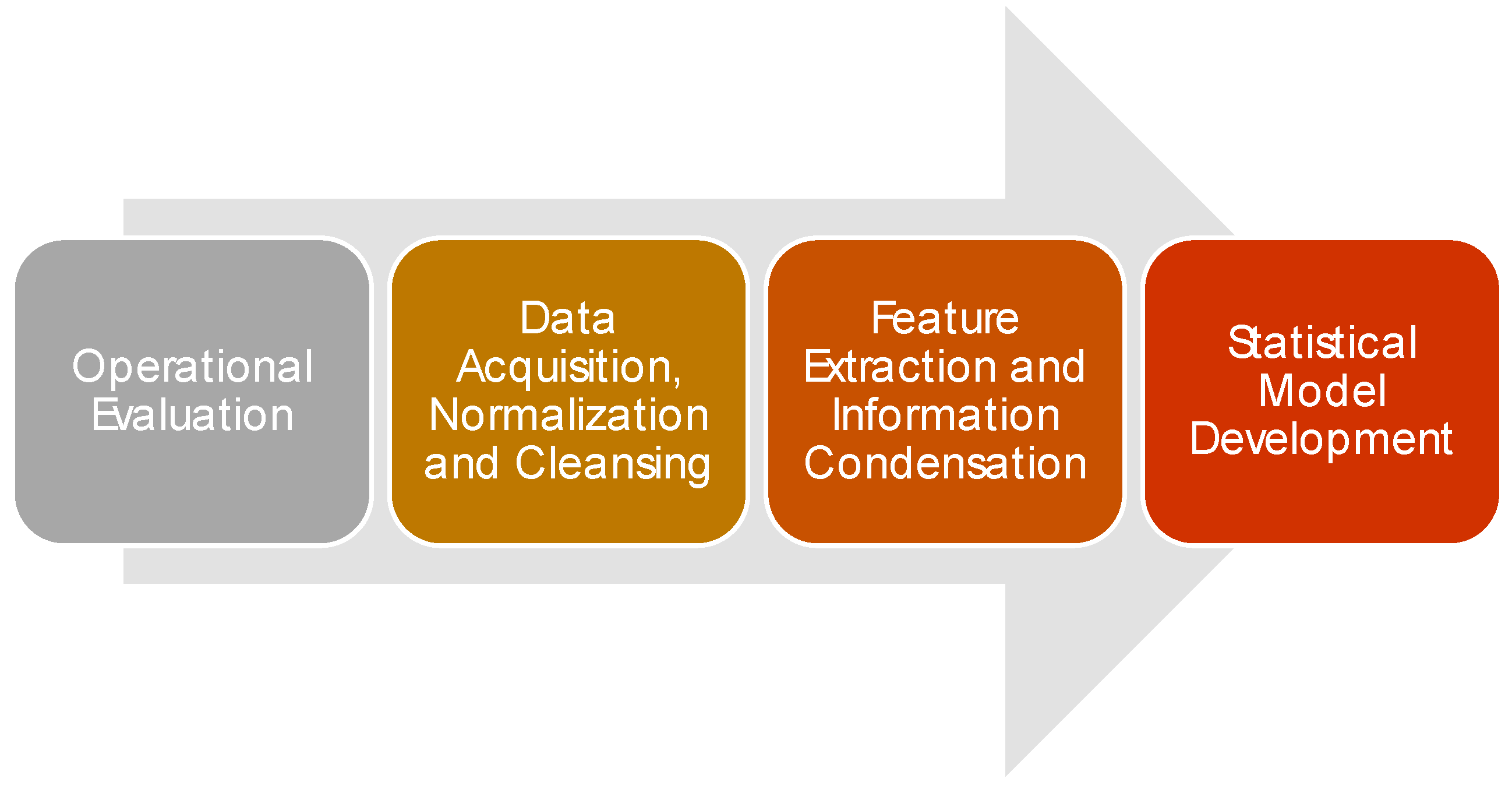
As previously mentioned, the SHM strategy for the through-life of an OWF should, ideally, be built during the design stage. This means that while some design milestones are settled (foundation type, pile depth, stiffness, natural frequency, different welds criticality, etc.), SHMS can be designed to cover risky aspects of the design and to optimise the inspection intervals. The way SHMS are designed and implemented follows the Statistical Pattern Recognition (SPR) paradigm, which is widely used across different industries for the implementation of damage detection strategies [35,36]. This paradigm was initially introduced in the SHM field by Farrar and Sohn [37] and later on adapted to the offshore wind industry by Martinez-Luengo et al. [38,39]. The SPR paradigm consists of four stages, which are intensively described in [38]. These stages are presented in Figure 1.

Operational evaluation is the first stage of the SPR paradigm and the one to be approached first during the design stage, as it sets the boundaries of the damage identification problem. This subsection focuses on the operational evaluation stage in order to give an example of the process and set the basis of the cost-benefit analysis carried out in Section 3. This stage aims to answer four questions concerning the implementation of the damage detection strategies. These questions relate to the following:

• The motivation and economic justification for implementing the SHMS: while the motivation for the implementation of SHMS is to gain certainty in the structural integrity of the monitored assets, extend the service life and increase the WF revenue, the economic justification is covered in the next Section with the cost-benefit analysis.
• The different systems’ damage definitions.
• The Environmental and Operational Conditions (EOC) in which the SHMS are used.

Operational evaluation, which is often disregarded in the literature, is crucial for the development of SHM strategies. It identifies the different failure mechanisms that are potentially worth monitoring and establishes damage thresholds. These damage thresholds are later employed to determine whether something is compromising the structural integrity of the assets, and therefore an unscheduled inspection is required to verify the extent of the damage and potentially carry out repair works, or everything is behaving as expected, and therefore a future scheduled inspection may not be required. The EOC in which the SHMS are operating also needs to be set in the operational evaluation stage (part C), as depending on the technologies employed, issues may arise with the damage sensitive features obtained (i.e., modal analysis).

In order to perform the operational evaluation, the basis for the next section’s cost-benefit analysis needs to be set. For this purpose, a baseline scenario for an OWF is defined. The main characteristics of this baseline case are given in

Table 4. WF baseline scenario and Environmental and Operational Conditions (EOCs).

Characteristic	Unit	Value
Number of OWTs	-	100
Turbine capacity	MW	5
WF area	km2	50
Average distance to port	km	50
Average water depth	m	30
Foundation type	-	Monopile
Number of offshore substations	-	1
Average wind speed	m/s	10.0 m/s (at hub height)
Tidal conditions	s	0.5m (HAT to LAT)
50 year wave	m	6.5
Current	m/s	1.0
Number of export cables	-	1

.

Based on these characteristics, the failure modes of the SS (foundation, GC and transition piece (TP)) are identified. After the failure mode identification, those failure modes that could potentially be monitored are analysed and their condition-based inspection strategy is optimised [40].

Table 5. Failure modes of wind turbine support structures and their effects on structure integrity.

Failure Mode	Impact on Structural Integrity	Can be Monitored?	SHMS
Cracks in welds	Accelerated fatigue	YES	Accelerometers and/or strain gauges
Corrosion	Loss of material leading to over-utilisation	YES	Impressed currents (ICCP)
Excessive fouling or marine growth	Corrosion and modification of modal properties and loading conditions	NO	Could be monitored by accelerometers but difficult to estimate the root cause of the modification in natural frequencies. Therefore it deems not worth monitoring
Scour	Loss of bearing capacity and modification of modal frequencies	YES	Accelerometers (not first mode), cameras or sonar
Grouted connection (GC) displacement	Loss of structural integrity	YES	Linear variable differential transformer (LVDT)

shows the effect that these failure modes may have on the structural integrity of the assets.

Accelerated fatigue can lead to collapse of the structure before its decommissioning, which is the reason why some OWFwere intentionally overdesigned. However, this overdesign implies a potential loss of revenue due to the decommissioning of an asset that may still be able to operate safely. Maximising return of investment (RoI) while optimising LCoE through the asset’s life extension could be achieved when the structural integrity of the aforementioned asset is well known. This is when continuous SHM becomes necessary. Fatigue and modal property monitoring are among the most important SHM techniques for SS of OWF, as the consequences of structural damage may be catastrophic. Modal properties can be monitored though the variation that modal parameters, such as resonance frequency, damping coefficient and modal curvatures, among others, experience with the change in different physical properties (i.e., reduction in mass or stiffness) [35,37]. In order to carry out modal property monitoring and analyse the structure’s dynamic response, several accelerometers must be installed [38]. Operational modal analysis (OMA) allows modal parameters in operational conditions to be estimated based only on vibration responses, without measuring the excitation forces [41,42].

Corrosion is one of the failure modes that most compromises the integrity of the SS of OWT, as it attacks any unprotected metal surface. This failure mechanism can be avoided by the protection of these surfaces in contact with the sea water [43]. Contact between dissimilar metals must also be avoided to prevent galvanic corrosion. This is achieved by the introduction of isolating elements and washers between the two metals [44]. The corrosion protection system of the SS of OWT comprises corrosion allowance, paint coating and cathodic protection by means of sacrificial anodes (SACP) or impressed currents (ICCP). All primary steelwork surfaces of the monopile and TP, the secondary steelwork and the main access platform elements are coated according to ISO 12944 [45]. The SACP consists of stand-off sacrificial anodes made of Al-Zn-In, cast onto a steel insert, which are welded onto the monopile structure. Corrosion is generally not monitored, although it can be done via ICCP. ICCP is an innovative method where direct current is used to regulate the cathodic protection of a structure based on the potential in the water [46]. Therefore, the use of an external power supply enables the operator (who must be constantly monitoring the voltage requirement) to adapt the current to the voltage requirements at any time. ICCP also generates significantly higher current output with fewer, longer lasting anodes than a conventional SACP system [46]. The main benefit ICCP possess is that anode depletion can be monitored and controlled. Therefore, the chances of failure of the cathodic protection of the asset are minimised [47].

ICCP costs are complicated to estimate. For that reason, ICCP has not been included in the SHM strategy for the baseline scenario of the cost-benefit analysis presented in Section 3. Only SACP, coating and corrosion allowances have been utilised for the corrosion protection of the assets. Typically, monopiles are designed with the intent of preventing internal corrosion, as wall thickness (and therefore CAPEX) would significantly increase if corrosion allowance was to be provided internally as well as externally. A way of preventing internal corrosion would be by sealing the internal compartments to eliminate the influence of oxygen and corrosive substances [48]. However, in the case of monopiles, this sealing strategy is challenged in several areas:

• The sealing around the cable entry and exit.
• The edges around the post-mounted airtight platform sealing the upper part of the monopile.
• The GC between the monopile and TP.

Due to these challenges, corrosion protection inside the monopile for this case study will be carried out by the implementation of SACP as opposed to coating, as SACP systems can be easily designed to last for the whole life of the structure (including decommissioning), whereas the expected lifetime of the coating is usually around 15 years.

One of the main challenges in the design and operation of OWT arises from the uncertainty of maximum scour depth around their foundations. Scour action can lead to excessive excavation of the surrounding seabed and is considered a major risk for OWF developments [49]. However, real-time scour data is currently not being collected by operators due to the lack of available instrumentation and monitoring techniques. New scour monitoring technologies for OWT installations are currently being investigated [50,51,52].

GC displacement is a dangerous failure mechanism as it compromises the overall integrity of the OWT SS but also the ability of the turbine to produce electricity. GC displacement occurs when the axial capacity of the connection between the grout and the TP or the grout and the monopile is insufficient, leading to a relative displacement between these elements and ultimately to the TP sliding down the monopile to the seabed. The cause of the lack of axial capacity potentially stems from a number of possible failure modes, which are described and analysed in [53]. GC displacement can be easily detected by the use of displacement sensors (i.e., linear variable differential transformer (LVDT)), indicating loss of capacity in the GC. The extent of the loss of axial capacity can also be determined by the installation of strain gauges in the stoppers of the TP. These stoppers are used temporarily during the installation of the TP. In the event that there is a loss of axial capacity, the TP would slide down until its stoppers rest on the monopile and carry some, or all, of the axial and bending loads from the wind turbine, which would be captured by the strain gauges.

According to BSH regulations, 10% of the SS in any German WF must be equipped with permanent SHMS or Condition Monitoring Systems (CMS). These systems should be planned in accordance to the risk identification and prioritisation previously carried out. Other aspects to be taken into account in the selection of the locations to be monitored include:

• Even monitoring of different structures within the OWF. Sometimes in an OWF not all the turbines have the same design or even the same manufacturer. This may occur when there is a high variation of water depths across the OWF, or a very high number or assets to be commissioned. Therefore, enough assets within each group of structures must be monitored in order to be able to ascertain whether SHM data represents a single turbine, a group of assets or the entire WF.
• Minimisation of the potential loss of production due to failure and consequent turned-off turbines close to the offshore substation, affecting the whole production of the array.
• Maximum water depth location due to highest seabed stresses produced by wave loading.
• Critical locations in accordance to manufacturing or installation deviations. Sometimes fabrication and installation do not happen as expected. When deviations occur, a better assessment of the asset’s integrity is recommended. Aside from the requirement specified in BSH standards, a higher number of assets may be equipped with permanent SHMS or CMS if deemed necessary.

Ideally all turbines (or as many as possible) should have the same SHMS or CMS installed so that conclusions and trends can be derived across the WF [39]. These SHMS or CMS must be reliable and have a relatively high service life. They should also be able to collect data for long time periods without the necessity of inspection and maintenance on site. Therefore, sufficient redundancy shall be provided at the hardware, the software and the data storage. For the SHM systems,

Table 6. SHM strategy: number, type and hardware location.

Sensor Type	Sensors/WT	At Levels	Sensors/10 WT
2D accelerometer	3	Top of TP, 2/3 of Tower height and Top of Tower	30
2D inclinometer	1	Top of TP	10
Displacement sensor (LVDT)	3	Bottom of TP at the stoppers	30
Strain gauges	12	4 sensors per level: Top of TP (external), bottom TP (stoppers), top of monopile	120
Temperature sensor	3	Top and Bottom of TP, top of monopile	30
Data acquisition unit	1	Inside TP	10

details the necessary hardware to be installed. This SHMS strategy is comprised of acceleration, inclination and temperature sensors. Ten out of the 100 locations have the base case SHMS complemented by strain gauges. This arrangement of sensors serves to evaluate the dynamic and static behaviour of the SS under the actual site conditions, acknowledging temperature effects.

2.3. Inspection Strategy

A structural inspection strategy for the SS service life at the WF level is developed in this subsection, following the requirements of the BSH. BSH legislation has been chosen as it is more restrictive than the one applying in the United Kingdom. This inspection strategy is fundamentally divided into two types of work—above water and below water—which is strongly related to the three different types of periodical inspections described in DNVGL-ST-0126 [34]. This division concerns the different personnel, equipment and logistics needed. The following activities are believed to be necessary in order to have confidence in the structural integrity of the assets.

2.3.1. Above Water

General visual inspection (GVI) of primary and secondary steel: The aim of this inspection is to provide a general overview of the integrity of the part of the SS that is above water. This involves a general inspection passing around the monopile and access systems from a crew transfer vessel (CTV). The objective is to identify any obvious mechanical, fatigue or corrosion damage. These damages could be manifested as cracks, plastic deformation, buckling, denting, generalised galvanic corrosion, pitting, dents in the coatings or excessive marine growth. Once the access systems have been cleared, the personnel must check the main access platform and TP.

Close visual inspection (CVI) of primary and secondary steel: The aim of this inspection is to detect corrosion or fatigue damage in the inspected areas of the TP, main access platform and access systems above water, and determine whether non-destructive testing (NDT) would be necessary to inspect any of the welds. This inspection is carried out closer to the structure (at a meter distance), therefore detecting smaller defects.

Detailed Visual Inspection (DVI) of primary and secondary steel: The aim of this inspection is to determine the extent of fatigue damage when cracks are detected at pre-selected welds. In order to achieve this NDT is employed. This inspection is carried out as a reactive measure when there is either a strong suspicion or evidence of fatigue damage being present at welds.

2.3.2. Below Water

Subsea GVI of primary and secondary steel: The aim of this inspection is to provide a general overview of the integrity of the part of the SS that is below water in the same way it is done above water. This inspection can be carried out by divers or by a remotely operated vehicle (ROV).

Subsea CVI of primary and secondary steel: The aim of this inspection is to identify corrosion or fatigue damage in the inspected areas of the TP and monopile below water, and determine whether NDT would be necessary to inspect any of the welds. This inspection is carried out at a meter distance. For these analyses, marine growth cleaning as well as good visibility and environmental conditions are required. The necessary equipment to carry out this inspection is an ROV, a water jet to clean the marine growth, a length measuring device and a camera to document findings.

Subsea DVI of primary and secondary steel: The aim of this inspection is to determine the extent of fatigue damage when cracks have been detected at pre-selected welds using NDT techniques. This inspection would be carried out as a reactive measure when there is either a strong suspicion or evidence of fatigue damage being present at welds.

CVI of the GC: The aim of this inspection is to assess the integrity of the GC between the TP and the monopile. “Eight o-clock” positions around the circumference of the bottom of the GC will be inspected and measurements will be taken at the level of the grout with regards to the bottom of the TP. Any evidence of grout material loss or surface cracks shall be reported. This inspection will be carried out by divers or an ROV.

Marine growth survey: The aim of this inspection is to estimate the coverage, thickness and type of marine growth colonisation on the monopile and sacrificial anodes and to compare its thickness against the one assumed in the design basis. Loading issues that could potentially arise from a significant deviation between the measurements and the design assumptions must be established [54]. Any marine growth formations on structural parts accessed by personnel, i.e., boat landings and access ladders, must be removed. This activity will be carried out either by divers or an ROV.

Cathodic protection survey: The aim of this inspection is to confirm if there is adequate global cathodic protection from the water table to the seabed. Potential readings are to be performed for every anode. Two methodologies can be followed to perform these readings: proximity readings using a reference electrode, and contact readings. Both of these methods consist of a cathodic protection probe to be mounted on an ROV. No cleaning of marine growth needs to be performed during this task, as this would disturb the measurements to be taken.

Scour survey: The aim of this inspection is to monitor changes in the seabed topology around the monopile foundation to account for both local and global scour. Seafloor objects and debris close to the structure must be identified and removed. Two different methods can be used: Multi Beam Echo Sounder Bathymetry Survey and Side Scan Sonar Survey.

3. Cost-Benefit Analysis

This Section investigates the potential impact that implementation of the SHM strategy presented in Section 2.2 will have on OPEX and the reduction of LCoE. For this reason, the variation in the scope of works of the inspection and maintenance plan throughout the life of the WF is estimated for three different scenarios (optimistic, average and pessimistic). For these scenarios, the reduction in OPEX of the OWF achieved by SHMS is assessed. OPEX accounts for any necessary expense incurred in the inspection, operation and maintenance of the offshore assets. OPEX usually consists of fixed costs that do not depend on the WF uptime and variable costs that depend on the time the WF operates [55]. Operations represent activities associated with high-level management of the plant, whereas inspection and maintenance are the tasks that entitle more effort, cost and risk. Inspection and maintenance can be preventive (carried out proactively before the system or component fails) or corrective (carried out once there has already been a failure that needs repair/replacing or the suspicion this failure is/will be developing). Unscheduled inspections and corrective maintenance take longer time to perform due to planning and logistics, the acquisition of spare parts, complexity of the repair and weather downtime. The longer these take to be performed, the higher the degradation of the system and the loss of production will be. One of the benefits of SHMS is that early onset of failures can potentially be detected, sometimes enabling preventive maintenance to be carried out, and other times enabling the mitigation of the consequences of such failures.

Inspection is the process where the assets are verified to be fit for purpose. For SS of OWT, these inspections check that none of the failure modes described in Table 5 pose a risk to the integrity of the structure. Offshore inspections are costly due to a number of factors, but mainly due to difficulties in the accessibility of the assets. That is the reason why relying on SHMS as an identification and diagnosis tool for failure mechanisms could help operators reduce the number of these inspections, and therefore OPEX. This Section calculates the potential saving in OPEX achieved by implementation of the SHM strategy in SS of OWF.

3.1. Scenarios

The main benefit of SHMS is that these systems, when applied effectively, can detect early stages of failure mechanisms being developed in the assets. The ability to react quickly to SHMS alarms helps mitigate these failure mechanisms and enables operators to have greater confidence in the structural integrity of their assets. This principle is explored in this section, where the added value of the implementation of SHMS in WTs is calculated. For this, the scenario presented in Section 2.2, where according to BSH only 10% of the assets are instrumented, is chosen as the baseline case. Furthermore, three other scenarios, including 20%, 30%, and 50% of instrumented assets, are considered. For all the scenarios, the inspection frequency is estimated depending on the number of instrumented assets, which is related to the operator’s confidence in the structural integrity of their assets. It should be noted that this confidence in the integrity status of the assets can be influenced by a number of factors, such as the global safety factor considered in their design, the operator’s experience in offshore wind O&M activities and the operator’s risk appetite.

The above-mentioned scenarios are presented in

Table 7. Scenarios of SHM implementation.

Activity	Baseline Scenario		Scenario 1		Scenario 2		Scenario 3
	SHMS in 10% of WTs	Inspection Frequency during Service Life	SHMS in 20% of WTs	Inspection Frequency during Service Life	SHMS in 30% of WTs	Inspection Frequency during Service Life	SHMS in 50% of WTs	Inspection Frequency during Service Life
GVI of primary and secondary steelwork	100% every year	25	100% every year	25	50% every year	12.5	20% every year	5
CVI of primary and secondary steelwork	25% every year	6.25	20% every year	5	15% every year	3.75	5% every year	1.25
DVI of primary and secondary steelwork	25% every year	6.25	20% every year	5	15% every year	3.75	5% every year	1.25
Seabed scour survey	100% the 2 first years and then 25% every year	7.75	100% the 2 first years and then 20% every year	6.6	100% the 2 first years and then 15% every year	5.45	100% the 2 first years and then 5% every year	3.15
Subsea marine growth survey	25% every year	6.25	20% every year	5	15% every year	3.75	5% every year	1.25
Cathodic protection potential survey	100% the 2 first years and then 25% every year	7.75	100% the 2 first years and then 20% every year	6.6	100% the 2 first years and then 15% every year	5.45	100% the 2 first years and then 5% every year	3.15
CVI of the GC	25% every year	6.25	20% every year	5	15% every year	3.75	5% every year	1.25
GVI of primary and secondary steelwork	25% every year	6.25	20% every year	5	15% every year	3.75	5% every year	1.25
CVI of primary and secondary steelwork	25% every year	6.25	20% every year	5	15% every year	3.75	5% every year	1.25
DVI of primary and secondary steelwork	25% every year	6.25	20% every year	5	15% every year	3.75	5% every year	1.25

, where the number of inspections performed on each one of the assets during their service life is specified following BSH regulations. This implies that for some of the activities, all the assets must be inspected in the first couple of years, with the interval between inspections able to be increased afterwards. Also, a higher number of instrumented turbines implies an increase in CAPEX due to the extra instrumentation and installation. The aim of this section is to calculate the added value of the implementation of SHMS in SS of OWF. This is achieved by the comparison of the reduction in OPEX versus the increase in CAPEX due to the implementation of higher percentages of SHMS from the three scenarios presented in Table 7.

3.2. CAPEX Increase Due to SHM Implementation

This sub-section evaluates the increase in CAPEX costs ($\Delta CAPEX$) incurred due to implementation of the SHM strategy under three scenarios of 20%, 30%, and 50% of instrumented assets. The cost of implementation of the SHM strategy (${\phi }_{SHM}$) is given by:

$$\Delta CAPEX={\phi }_{SHM}={\phi }_H+{\phi }_V+{\phi }_I+{\phi }_M+{\phi }_{PM}$$

(1)

Hardware costs (${\phi }_H$) are related to the sensors, cabling, and data acquisition units (DAU) required for the implementation of these systems. The cost of the necessary hardware for applying the SHM strategy (developed in Section 2.2) to the Baseline case under the scenarios 1, 2 and 3 is detailed in

Table 8. Hardware costs in Baseline scenario.

Sensor Type	Sensors/WT	Average Unit Rate (€)	Ref.	Total Number of Sensors	Average Cost
2D Accelerometer	3	621.5	[56,57]	30	36,000
2D Inclinometer	1	661.5	[58,59]	10	10,000
Displacement sensor (LVDT)	3	167.5	[60,61]	30	6450
Strain gauges	12	105.25	[62,63]	120	12,000
Temperature Sensor	3	182.25	[64,65]	30	4200
DAU	1	6988.5	[66,67]	10	115,000

.

Installation and calibration cost (${\phi }_I$) is another cost incurred by the implementation of SHMS. This cost accounts for installation and calibration activities that are typically subcontracted to either the hardware supplier or a service provider. Personnel costs are also accounted for by ${\phi }_I$. When third parties are involved, there are other costs associated with SHMS, such as the mobilisation and demobilisation costs (${\phi }_M$), vessel cost (${\phi }_V$), and project management costs (${\phi }_{PM}$); ${\phi }_M$ is related to the cost incurred by the third party for travelling personnel and transporting goods for the duration of the works. This is highly variable with the duration of the installation, the number of personnel taking part in the works and the geographic location of the WF.

Table 9. Mobilisation and demobilisation costs for the different scenarios.

Scenario	People	Days	Cost (k€)
Baseline	4	10	14
Scenario 1	8	10	28
Scenario 2	12	10	42
Scenario 3	20	10	70

shows the number of people considered to take part in the installation of the hardware; ${\phi }_I$ and ${\phi }_M$ are estimated by using the following equations:

$${\phi }_I=0.3 {\phi }_H$$

(2)

$${\phi }_M=350\frac{€}{person\ast day}$$

(3)

Depending on the nature of the monitoring campaign, the installation could be carried out either onshore or offshore. Typically, performing the same type of work could be up to ten times more expensive if performed offshore rather than onshore [68]. Therefore, given the fact that these systems are implemented from the commissioning stage, their installation would be carried out onshore. Therefore, no ${\phi }_V$ is incurred this time.

The ${\phi }_{PM}$ is related to all administration and coordination activities to make the installation of the SHMS possible. These costs tend to vary depending on the supplier, and therefore have been estimated from the following formula extracted from [69]:

$${\phi }_{PM}=0.03\ast \left({\phi }_H+{\phi }_V+{\phi }_I+{\phi }_M\right)$$

(4)

3.3. OPEX Reduction Due to SHM Implementation

This sub-section investigates the reduction in OPEX achieved by implementation of the SHMS strategy. As the number of instrumented turbines increases, the knowledge and certainty about the structural integrity of the assets also rises. This enables the operators to reduce the number of inspections carried out on the assets throughout their service life. It is believed that the decrease in OPEX due to the reduction in the number of inspections exceeds the increase in CAPEX due to the cost associated with instrumenting the units. In this sub-section, the OPEX reduction due to SHM implementation is calculated. Inspection costs are influenced by the following aspects:

• Cost of accessibility $\left({\phi }_A\right)$: how many turbines can be inspected in a day, depending on the type of inspection to be carried out, type of vessel to be used $\left({\phi }_V\right)$, commuting time to the WF and back, fuel consumption of the vessels, price of fuel, etc.
• Equipment costs, depending on each activity $\left({\phi }_E\right)$.
• Personnel costs $\left({\phi }_P\right)$: how many people intervene, their daily rate and their shifting patterns.
• Project management costs $\left({\phi }_{PM}\right)$: to account for logistics organization and reporting.

Accessibility has a great influence on the cost of inspections. Depending on where the activity is carried out (above water or below water), a certain type of vessel is employed. Typically, there are two options: CTV and service vessel (SV). CTVs are designed to be efficient and effective. They are specially designed to work in the OW sector. CTVs are generally small aluminum catamarans employed to transfer personnel in and out of offshore sites on a daily basis [70]. Their carrying capacity is usually 12 crew who do 12-hour shifts, meaning that the CTV would come back to port by the end of the day. Transit speeds range between 15 and 30 knots [70]. SVs are boats designed, modified, or equipped to carry out sea mapping. SVs are generally equipped with Sidescan Sonar or Multibeam Echosounder. They are employed for subsea operations, as generally CTVs do not have the capability to launch an ROV or enough dynamic positioning redundancies to keep still during the ROV operation. These vessels have a capacity of around 10 passengers and they perform 24-hour operations, which means that they would only come back to port approximately once every two weeks [71]. They are bigger and slower than CTVs, with cruising speeds around 20 knots when they are half-loaded [72].

Table 10. Vessel costs.

$\mathbf{Vessel}\mathbf{Cost}\left({\mathit{\phi }}_{\mathit{V}}\right)$	CTV	SV	Reference
mob/demob (€)	0	70,000	[73]
day rate (€/day)	3700	5000

shows mobilization and demobilisation costs and daily rates for both CTVs and SVs.

Regarding the amount of turbines that can be inspected in a day, the actual number not only depends on the inspection to be carried out, but also on the transit time to the site for above water works and on the transit time between turbines for both above and below water works. These transfers have been estimated and are shown in

Table 11. Average transit times and cost.

Average transit time to OWF (hr)	1.5
Average transit time to turbine (hr)	0.25
Average fuel consumption (L/ Nautical Mile)	25
Average cost of fuel (€/L)	0.6

.

Table 12. Equipment costs.

$\mathbf{Equipment}\mathbf{Cost}\left({\mathit{\phi }}_{\mathit{E}}\right)$	Day Rates (€/day)	Source
Mechanical toolkit	50	[74]
ROV	2750
measuring toolkit	500
NDT equipment	700
Water jet	0	[75]

shows equipment costs and their daily rates for inspection of SS in OWF.

Table 13. Activities specifications: vessel type, personnel, working time and equipment.

Work Package	Activity	Vessel Type	Personnel	Shift Type	hr/WT (Average)	Equipment	WT/Day (Average)
AW	GVI of primary and secondary steelwork	CTV	2	12	1.5	Mechanical toolkit	5
AW	CVI of primary and secondary steelwork	CTV	2	12	2.5	Mechanical toolkit	3
AW	DVI of primary and secondary steelwork	CTV	2	12	4	NDT equipment	2
SB	Seabed scour survey	SV	10	24	1.75	Geophysical survey equipment	11
SB	Subsea marine growth survey	SV	10	24	1.5	ROV and measuring toolkit	12
SB	Cathodic protection potential survey	SV	10	24	3	ROV and measuring toolkit	7
SB	CVI of the GC	SV	10	24	2	ROV and measuring toolkit	9
SB	Subsea GVI of primary and secondary steelwork	SV	10	24	2	ROV	9
SB	Subsea CVI of primary and secondary steelwork	SV	10	24	7	ROV, measuring toolkit, water jet and NDT equipment	3
SB	Subsea DVI of primary and secondary steelwork	SV	10	24	6	ROV, measuring toolkit and water jet	3

shows the estimation of time that each one of the inspections takes and the number of turbines that can be inspected by the end of the day. It must be noted that this time is subject to variations depending on the details of inspection activities, technicians’ experience, environmental conditions, etc. Table 13 shows the amount of personnel required for each inspection and the necessary equipment to be deployed. It should be noted that “solo working” is not permitted due to H&S considerations. Also, to account for the 24-hour works below water without returning to port for periods of sometimes up to two weeks, the working crew would be on average 10 passengers [76]. Personnel salary highly depends on the project, geographic location and qualifications. In a previous study [73], personnel salary $\left({\phi }_P\right)$ is reported to be 270 £/day (around 310 €/day), however, from the authors’ point of view, this salary might be up to twice as much.

3.4. Sensitivity Analysis

Inspection costs are subject to uncertainties due to the large number of factors and stakeholders involved in these activities. To this aim, a sensitivity analysis is performed to evaluate the effect of two factors on CAPEX and OPEX. These two factors are: cost of SHM hardware and inspection time. Nowadays, various sensors with a range of prices are available in the offshore wind energy market.

Table 14. Sensitivity analysis of hardware price.

Sensor Type	Unit Price (€) (Optimistic)	Unit Price (€) (Average)	Unit Price (€) (Pessimistic)
2D Accelerometer	160	621.5	1083
2D Inclinometer	293	661.5	1030
Displacement sensor (LVDT)	95	167.5	240
Strain gauges	43	105.25	167.5
Temperature sensor	110.5	182.25	254
DAU	1037	6988.5	12,940

presents an optimistic, average and pessimistic range of hardware prices. As can be observed, for a sensor with similar specifications, there might be up to a 100% increase in price due to slight modifications in the design. The effect of these fluctuations on the increase of CAPEX due to the instrumentation of a higher percentage of assets is investigated.

Inspection time is another variable aspect that strongly influences the cost of inspection campaigns. Inspection time is susceptible to weather conditions, sea state, technicians’ experience, condition of the asset, etc. An increase in inspection time leads to an increase in the number of offshore days within a campaign. This may not seem crucial, however, this time-increase has other associated costs, such as deployment of a vessel, personnel, and equipment offshore. Furthermore, inspection times may vary depending on the supplier performing the activities. A 30% weather downtime has been considered in these analyses.

Table 15. Sensitivity analysis of inspection time.

Activity	hrs/WT (Optimistic)	hrs/WT (Average)	hrs/WT (Pessimistic)	WT/Day (Optimistic)	WT/Day (Average)	WT/Day (Pessimistic)
GVI of primary and secondary steelwork	1	1.5	2	8	6	5
CVI of primary and secondary steelwork	1.5	2.5	3.5	6	4	3
DVI of primary and secondary steelwork	3	4	5	3	3	2
Seabed scour survey	1	1.75	2.5	17	11	8
Subsea marine growth survey	1	1.5	2	17	13	10
Cathodic protection potential survey	2	3	4	10	7	5
CVI of the GC	1	2	3	17	10	7
Subsea GVI of primary and secondary steelwork	1	2	3	17	10	7
Subsea CVI of primary and secondary steelwork	6	7	8	4	3	3
Subsea DVI of primary and secondary steelwork	4	6	8	5	4	3

shows the optimistic, average and pessimistic scenarios used for the sensitivity analysis of this case study and how the increase or decrease in time to perform the different inspections influence the number of assets to be inspected in a single working day.

4. Results and Discussion

In this Section, the results of the cost-benefit analysis are reported. The aim is to quantify the added value of SHMS when implemented from the installation of the OWF. The total CAPEX is £1.68 billion (around €1.87 billion), while the annual OPEX was estimated at £56.6 million (around €63 million) [73]. With the implementation of SHM,

Table 16. SHMS cost and CAPEX % for hardware sensitivity analysis.

Scenario	SHM Cost and Hardware Cost Sensitivity Analysis
	Optimistic		Average		Pessimistic
	Cost (M€)	CAPEX %	Cost (M€)	CAPEX %	Cost (M€)	CAPEX %
Baseline	0.04	0.003	0.16	0.009	0.28	0.016
Scenario 1	0.08	0.006	0.32	0.019	0.55	0.031
Scenario 2	0.12	0.009	0.48	0.028	0.83	0.047
Scenario 3	0.20	0.014	0.79	0.046	1.39	0.078

shows the CAPEX increase due to the SHM implementation for the baseline scenario and scenarios 1, 2 and 3. Furthermore, the results of the sensitivity analysis performed with regards to the highly variable hardware prices are given in Table 16. As can be appreciated, the hardware cost variation plays an important role in the overall cost of implementation and subsequent CAPEX increase. It can be observed that CAPEX increase in an “optimistic scenario 3” (SHMS in 30% of the assets) is 25% cheaper than an “average Baseline scenario” (SHMS in 10% of the assets).

These results suggest that hardware selection and acquisition constitutes a very important aspect of SHM implementation. Figure 2, Figure 3 and Figure 4 show the amount of increase in CAPEX due to SHM implementation in Scenario 3 for three cases of optimistic, average and pessimistic hardware costs respectively. As can be seen in the figures, the cost of SHM implementation accounts for a small proportion of the total CAPEX.

Overall, it can be concluded that the percentage of CAPEX increase when SHMS are installed onshore is less than 0.1% of the CAPEX. The quantification of the OPEX percentage dedicated to structural inspections of the assets throughout their lifetime is given in

Table 17. Lifetime inspection costs and inspection-time sensitivity analysis for Baseline case, Scenario 1, 2 and 3.

Scenario	Inspection Time Sensitivity Analysis
	Optimistic		Average		Pessimistic
	Cost (M€)	OPEX %	Cost (M€)	OPEX %	Cost (M€)	OPEX %
Baseline	15.6	1.2	19.9	1.6	24.4	1.9
Scenario 1	13.1	1.0	16.8	1.3	20.5	1.6
Scenario 2	9.5	0.8	12.1	1.0	14.9	1.2
Scenario 3	3.8	0.3	4.9	0.4	6.1	0.5

and is graphically shown in Figure 5. The results of the sensitivity analysis performed on the effect of inspection time in the cost of inspections and OPEX are also presented in Table 17.

Furthermore,

Table 18. Lifetime OPEX reduction due to SHM implementation and inspection time.

Scenario	OPEX Reduction for Different Inspection-Time Scenarios
	Optimistic		Average		Pessimistic
	M€	%	M€	%	M€	%
Scenario 1	2.5	0.2	3.2	0.3	3.9	0.3
Scenario 2	6.1	0.5	7.8	0.6	9.5	0.8
Scenario 3	11.8	0.9	15.0	1.2	18.3	1.5

shows the OPEX percentage reduction in terms of structural inspection costs for the three cases of optimistic, average and pessimistic inspection time under different SHM implementation scenarios when compared to the baseline case. Even though the percentages are low (below 2%), they represent up to 18.3 M€. It is worth mentioning that these savings took into account scheduled inspection and maintenance but unscheduled activities were ignored, which given their often urgent nature will increase OPEX considerably. The reason why unscheduled inspection and maintenance has not been considered in the study is the lack of available data in the literature.

Table 18 and Figure 6 show the reduction of OPEX due to the implementation of SHMS in the WF. Furthermore, Figure 6 presents graphically how the lifetime cost of each one of the different inspections decreases with the number of times such inspections are performed to all the assets in their lifetime. This is related to the different scenarios presented in Table 7, where a higher percentage of SHM implementation enhanced the confidence in the structural integrity of the assets, enabling a smaller frequency of inspection. Thus, in Figure 7, while average inspection-time scenarios are represented by different symbols in the legend, optimistic and pessimistic scenarios are shown by dashed lines. These optimistic and pessimistic inspection-time scenarios represent the upper and lower bound of the cost interval, respectively. Furthermore, Figure 7 shows the cost reduction when the number of lifetime inspections is reduced due to SHM implementation. Slope change between above/below water inspections can be observed.

Lastly,

Table 19. CAPEX increase versus OPEX reduction due to SHMS implementation.

SHM Implementation Scenario	Hardware Cost Sensitivity Analysis	Inspection-Time Sensitivity Analysis
		Optimistic		Average		Pessimistic
		CAPEX Increase (M€)	OPEX Reduction (M€)	CAPEX Increase (M€)	OPEX Reduction (M€)	CAPEX Increase (M€)	OPEX Reduction (M€)
Scenario 1	Optimistic	0.08	2.48	0.08	3.16	0.08	3.87
	Average	0.32		0.32		0.32
	Pessimistic	0.55		0.55		0.55
Scenario 2	Optimistic	0.12	6.12	0.12	7.81	0.12	9.51
	Average	0.48		0.48		0.48
	Pessimistic	0.83		0.83		0.83
Scenario 3	Optimistic	0.20	11.78	0.20	15.03	0.20	18.31
	Average	0.79		0.79		0.79
	Pessimistic	1.39		1.39		1.39

summarizes the increase in CAPEX versus the decrease in OPEX that different SHM implementation scenarios have for the optimistic, average and pessimistic cases of both sensitivity analyses for SHM hardware cost and inspection time. As can be appreciated, SHM implementation makes sense in all of the cases, as the OPEX reduction is much higher than the CAPEX increase due to the implementation of the SHMS. From Table 19 it can be concluded that the added value of SHM implementation ranges from 1.93–18.11 M€ for the presented scenarios and sensitivity analyses. Therefore, it can be concluded that SHM implementation can help WF operators reduce LCoE and maximise RoI.

5. Conclusions

In this paper, guidelines for the implementation of an SHMS were developed and applied to a case study. SHMS, when installed from the beginning of operation of the WF, can be used to adopt a condition-based inspection strategy for reducing OPEX. The regulations to be adhered to for the specific cases of the United Kingdom and Germany were extensively described and then the process to be followed by operators for the development of a SHM strategy together with an inspection strategy was explained and applied to a baseline case study. This baseline case study was used to perform the economic analysis of the benefits of SHMS implementation in the reduction of OPEX based on the developed guidelines.

Results back up the hypothesis that when implemented from the beginning of the service life, SHMS help WF operators reduce the number of necessary inspections required, thereby reducing OPEX. This reduction was found to be much greater than the cost associated with the implementation of these systems. Furthermore, hardware selection and acquisition constitute a very important aspect of SHM implementation, whilst this cost remains significantly lower than the total CAPEX. Thus, the percentage of CAPEX increase due to SHMS implementation remains less than 0.1% of CAPEX, whereas the percentage of OPEX reduction is estimated to be in the 0.2–1.5% range. Finally, the added value of SHM implementation was estimated to be between 1.93–18.11 M€ for the presented scenarios and sensitivity analyses.

An aspect that has not been taken into account due to the high variability and lack of economic data available was the unscheduled inspections and repairs in the structure of the OWT. The main benefit and the reason why inspections are scheduled less often when SHMS are implemented is that these systems are able to detect and sometimes predict failures. Therefore, by the implementation of these systems, unscheduled repairs with a subsequent loss of production are less likely to occur, which would be translated into a further reduction in OPEX. This idea is expected to be researched in further works.

References

1. BVG-Associates; WindEurope. Unleashing Europe’s Offshore Wind Potential; BVG-Associates: Swindon, UK, 2017. [Google Scholar]
2. WindEurope. Offshore Wind in Europe: Key Trends and Statistics 2017; WindEurope: Brussels, Belgium, 2017. [Google Scholar]
3. European Commission. Communication from the Commission to the European Parliament, the Council, the European Economic and Social Committee and the Committee of the Regions. Available online: http://ec.europa.eu/europe2020/pdf/europe2020stocktaking_en.pdf (accessed on 3 August 2017).
4. EWEA Business Intelligence. Aiming High: Rewarding Ambition in Wind Energy; The European Wind Energy Association: Brussels, Belgium, 2015. [Google Scholar] [CrossRef]
5. The Crown Estate. Offshore Wind—Operational Report 2017; The Crown Estate: London, UK, 2017. [Google Scholar] [CrossRef]
6. Leanwind. Driving Cost Reductions in Offshore Wind. 2018. Available online: https://windeurope.org/about-wind/reports/driving-cost-reductions-offshore-wind/ (accessed on 24 March 2019).
7. NewEnergyUpdate. Europe’s New Record Offshore LCoE Forecast at 40 Euros/MWh 2018. Available online: http://newenergyupdate.com/wind-energy-update/europes-new-record-offshore-lcoe-forecast-40-eurosmwh (accessed on 10 August 2018).
8. Daum, W. Guidelines for Structural Health Monitoring. In Handbook of Technical Diagnostics; Springer: Berlin, Germany, 2013. [Google Scholar] [CrossRef]
9. ISIS Canada—The Canadian Network of Canada. Guidelines for Structural Health Monitoring—Design Manual No. 2; ISIS Canada Corporation: Winnipeg, MB, Canada, 2001. [Google Scholar]
10. SAMCO. F08b Guideline for Structural Health Monitoring; SAMCO: Berlin, Germany, 2006. [Google Scholar]
11. Aktan, A.E.; Catbas, F.N.; Grimmelsman, K.A.; Pervizpour, M. Development of a Model Health Monitoring Guide for Major Bridges; Federal Highway Administration Research and Development: McLean, VA, USA, 2002. Available online: http://www.di3.drexel.edu/DI3/Events/PaperPresentation/ExeSumFHWA-|Longer%20Version.pdf (accessed on 13 March 2019).
12. Norsok Standard. N-005. Condition Monitoring of Loadbearing Structures; Norwegian Technology Standards Institution: Oslo, Norway, 1997. [Google Scholar]
13. Automatisierte Dauerüberwachung im Ingenieurbau; German Society for non-destructive testing City: Berlin, Germany, 2000; Available online: http://www.dgzfp.de/dienste/publikationen?kategorie=Zur%C3%BCckgezogen (accessed on 24 March 2019).
14. Lloyd, G. Guidelines for the Certification of Condition Monitoring Systems for Wind Turbines; Bereich Windenergie: Hamburg, Germany, 2007. [Google Scholar]
15. DECC. The Department for Energy & Climate Change. Organ Website. 2019. Available online: https://www.energy.gov/science-innovation/climate-change (accessed on 30 January 2019).
16. BSH. Bundesamt für Seeschifffahrt und Hydrographie. Organ Website, 2019. Available online: https://www.bsh.de/DE/Home/home_node.html (accessed on 30 January 2019).
17. Bundesamt für Seeschifffahrt und Hydrographie (BSH). Minimum Requirements Concerning the Constructive Design of Offshore Structures within the Exclusive Economic Zone; BSH: Hamburg, Germany, 2015. [Google Scholar]
18. Bundesamt für Seeschifffahrt und Hydrographie. Design of Offshore Wind Turbines; BSH: Hamburg, Germany, 2015. [Google Scholar]
19. Bundesamt für Seeschifffahrt und Hydrographie. Minimum Requirements for Geotechnical Surveys and Investigations into Offshore Wind Energy Structures, Offshore Stations and Power Cables; BSH: Hamburg, Germany, 2015. [Google Scholar]
20. Bundesamt für Seeschifffahrt und Hydrographie. Investigation of the Impacts of Offshore Wind Turbines on the Marine Environment (StUK4); BSH: Hamburg, Germany, 2015. [Google Scholar]
21. ISO. ISO 19901-6. Petroleum and Natural Gas Industries—Specific Requirements for Offshore Structures—Part 6: Marine Operations; ISO: Geneva, Switzerland, 2009. [Google Scholar]
22. ISO. ISO 19905-1. Petroleum and Natural Gas Industries—Site-Specific Assessment of Mobile Offshore Units—Part 1: Jack-Ups; ISO: Geneva, Switzerland, 2016. [Google Scholar]
23. ISO. ISO 29400. Ships and Marine Technology—Offshore Wind Energy—Port and Marine Operations; ISO: Geneva, Switzerland, 2015. [Google Scholar]
24. European Standard. EN 1990. Eurocode—Basis of Structural Design; The European Union: Bruxelles, Belgium, 2005. [Google Scholar]
25. European Standard. EN 1997. Eurocode 7—Geotechnical Design; The European Union: Bruxelles, Belgium, 2008. [Google Scholar]
26. European Standard. EN 1993-1-6 Eurocode 3—Design of Steel Structures—Part 1-6: Strength and Stability of Shell Structures; The European Union: Bruxelles, Belgium, 2007; Volume 6. [Google Scholar]
27. DET NORSKE VERITAS (DNV). DNV-OS-H101. Marine Operations, General; DNV: Akershus, Norway, 2011. [Google Scholar]
28. Germanischer Lloyd SE. GL-IV-7. Rules for Certification and Construction IV Industrial Services, Part 7 Offshore Substations; Germanischer Lloyd SE: Hamburg, Germany, 2013. [Google Scholar]
29. Germanischer Lloyd SE. GL-IV-6. GL Rules for the Certification and Construction, IV Industrial Services, Part 6 Offshore Technology; Germanischer Lloyd SE: Hamburg, Germany, 2013. [Google Scholar]
30. American Petroleum Institute Recommended Practice. API RP-2A-WSD Planning, Designing and Constructing Fixed Offshore Platforms—Working Stress Design; American Petroleum Institute: Washington, DC, USA, 2014. [Google Scholar]
31. Germanischer Lloyd SE. GL-IV-2. GL Rules and Guidelines, IV Industrial Services, Part 2 Guideline for the Certification of Offshore Wind Turbines; Germanischer Lloyd SE: Hamburg, Germany, 2005. [Google Scholar]
32. DET NORSKE VERITAS (DNV). DNV (Det Norske Veritas). DNV−OS−J101 Design of Offshore Wind Turbine Structures; DNV: Akershus, Norway, 2014. [Google Scholar]
33. DET NORSKE VERITAS (DNV). DNV-OS-J201. Offshore Substations for Wind Farms; DNV: Akershus, Norway, 2013. [Google Scholar]
34. DET NORSKE VERITAS (DNV). DNVGL-ST-0126. Support Structures for Wind Turbines; DNV: Akershus, Norway, 2016. [Google Scholar]
35. Farrar, C.R.; Worden, K. An introduction to structural health monitoring. Philos. Trans. A Math. Phys. Eng. Sci. 2007, 365, 303–315. [Google Scholar] [CrossRef] [PubMed] [Green Version]
36. Farrar, C.R.; Doebling, S.W. Damage Detection and Evaluation II. In Modal Analysis and Testing; Springer: Dordrecht, The Netherlands, 1999; pp. 345–378. [Google Scholar] [CrossRef]
37. Farrar, C.R.; Sohn, H. Pattern Recognition for Structural Health Monitoring; Los Alamos National Laboratory: Los Alamos, NM, USA, 2000.
38. Martinez-Luengo, M.; Kolios, A.; Wang, L. Structural health monitoring of offshore wind turbines: A review through the Statistical Pattern Recognition Paradigm. Renew. Sustain. Energy Rev. 2016, 64. [Google Scholar] [CrossRef]
39. Martinez-Luengo, M.; Shafiee, M.; Kolios, A. Data management for structural integrity assessment of offshore wind turbine support structures: Data cleansing and missing data imputation. Ocean Eng. 2019, 173, 867–883. [Google Scholar] [CrossRef]
40. Martinez Luengo, M.; Kolios, A. Failure Mode Identification and End of Life Scenarios of Offshore Wind Turbines: A Review. Energies 2015, 8, 8339–8354. [Google Scholar] [CrossRef] [Green Version]
41. Devriendt, C.; Magalhaes, F.; Weijtjens, W.; De Sitter, G.; Cunha, A.; Guillaume, P. Structural Health Monitoring of offshore wind turbines using automated operational modal analysis. Struct. Health Monit. 2014, 13, 644–659. [Google Scholar] [CrossRef]
42. Dong, X.; Lian, J.; Wang, H.; Yu, T.; Zhao, Y. Structural vibration monitoring and operational modal analysis of offshore wind turbine structure. Ocean Eng. 2018, 150, 280–297. [Google Scholar] [CrossRef]
43. Adedipe, O.; Brennan, F.; Kolios, A.J. Review of Corrosion Fatigue in Offshore Structures: Present Status and Challenges in the Offshore Wind Sector. Renew. Sustain. Energy Rev. 2016, 61, 141–154. [Google Scholar] [CrossRef]
44. Adedipe, O.; Brennan, F.; Kolios, A.J. Corrosion fatigue crack growth in offshore wind monopile steel HAZ material. In Proceedings of the 5th International Conference on Marine Structures (MARSTRUCT 2015), Southampton, UK, 25–27 March 2015. [Google Scholar]
45. International Organization for Standardization. ISO 12944 Paints and Varnishes. Corrosion Protection of Steel Structures by Protective Paint Systems; ISO: Geneva, Switzerland, 2018. [Google Scholar]
46. Kim, Y.; Seok, S.; Lee, J.; Lee, S.K.; Kim, J. Engineering Analysis with Boundary Elements Optimizing anode location in impressed current cathodic protection system to minimize underwater electric field using multiple linear regression analysis and artificial neural network methods. Eng. Anal. Bound. Elem. 2018, 96, 84–93. [Google Scholar] [CrossRef]
47. Jang, S.; Han, M.; Kim, S. Electrochemical characteristics of stainless steel using impressed current cathodic protection in seawater. Trans. Nonferrous Met. Soc. China 2009, 19, 930–934. [Google Scholar] [CrossRef]
48. DET NORSKE VERITAS (DNV). DNVGL-RP-0416. Corrosion Protection for Wind Turbines; DNV: Akershus, Norway, 2016. [Google Scholar]
49. Boon, J.D.; Sutherland, J.; Whitehouse, R. Scour behaviour and scour protection for monopile foundations of offshore wind turbines. Eur. Wind Energy 2004, 1–14. Available online: https://www.researchgate.net/profile/James_Sutherland/publication/228691951_Scour_behaviour_and_scour_protection_for_monopile_foundations_of_offshore_wind_turbines/links/54db3c0c0cf2ba88a68f7ee5/Scour-behaviour-and-scour-protection-for-monopile-foundations-of-offshore-wind-turbines.pdf?origin=publication_detail (accessed on 26 March 2019).
50. Martinez-Luengo, M.; Kolios, A.; Wang, L. Parametric FEA modelling of Offshore Wind Turbine Support Structures: Towards scaling-up and CAPEX reduction. Int. J. Mar. Energy 2017, 19, 16–31. [Google Scholar] [CrossRef]
51. Gupta, S.; Stoddart, E.; Sanderson, D.; Morrison, A. Condition monitoring of offshore wind turbines with scour and grout damage in monopile foundations. In Proceedings of the SECED 2015 Conference: Earthquake Risk and Engineering towards a Resilient World, Cambridge, UK, 9–10 July 2015. [Google Scholar]
52. Michalis, P.; Saafi, M.; Judd, M. Capacitive Sensors for Offshore Scour Monitoring. Energy 2013, 166, 189–197. [Google Scholar] [CrossRef]
53. Schaumann, P.; Raba, A.; Bechtel, A. Fatigue behaviour of grouted connections at different ambient conditions and loading scenarios. Energy Proc. 2017, 137, 196–203. [Google Scholar] [CrossRef]
54. Martinez-Luengo, M.; Causon, P.; Gill, A.B.; Kolios, A.J. The effect of marine growth dynamics in offshore wind turbine support structures. In Progress in the Analysis and Design of Marine Structures; CRC Press/Balkema: Leiden, The Netherlands, 2017; pp. 889–898. [Google Scholar] [CrossRef]
55. Ioannou, A.; Angus, A.; Brennan, F. Stochastic Prediction of Offshore Wind Farm LCOE through an Integrated Cost Model. Energy Procedia 2017, 107, 383–389. [Google Scholar] [CrossRef]
56. Omni Instruments Ltd. Subsea Acceleration and Vibration Logger. Available online: http://www.omniinstruments.co.uk/subsea-offshore-systems/subsea-logging-systems-and-displays/subsea-acceleration-and-vibration-logger.html (accessed on 5 December 2018).
57. Omni Instruments Ltd. Triple Axis Low Noise MEMS Accelerometer. Available online: https://www.omniinstruments.co.uk/catalogsearch/result/index/?dir=asc&limit=25&order=price&q=accelerometer (accessed on 5 December 2018).
58. Omni Instruments Ltd. G-NSDQL-004. DQG Series Dual-Axis Inclinometer. Available online: http://www.omniinstruments.co.uk/displacement-position-sensors/tilt-sensors/dqg-series-inclinometer.html (accessed on 5 December 2018).
59. Ltd LD. LSOC-3-A—LSO Inclinometer Sensor, ±3°, Output ±5 V. Available online: https://www.leveldevelopments.com/products/inclinometers/inclinometer-sensors/lsoc-3-a-lso-inclinometer-sensor-3-output-5v/ (accessed on 5 December 2018).
60. Electronics D-K. LVDT Transducers. Available online: https://www.digikey.es/products/en/sensors-transducers/lvdt-transducers-linear-variable-differential-transformer/522?utm_adgroup=Sensors+%26+Transducers&mkwid=sPyF8Bumv&pcrid=268479553667&pkw=&pmt=b&pdv=c&productid=&slid=&gclid=EAIaIQobChMIi9etuP7g3gIV77D (accessed on 3 December 2018).
61. Omni Instruments Ltd. Industrial Series LVDT. Available online: http://www.omniinstruments.co.uk/displacement-position-sensors/linear-position-and-lvdt-sensors/industrial-series-linear-velocity-displacement-transducers.html#partbuilder (accessed on 3 December 2018).
62. OMEGA Engineering. SGD-2/350-RY51. 3-Element Strain Gauge Rosette Triaxial: 0°/45°/90°. Available online: https://www.omega.co.uk/pptst/SGD_TRIAXIAL.html (accessed on 3 December 2018).
63. OMEGA Engineering. SGD-1.5/120-LY11 Linear Strain Gauges. Available online: https://www.omega.co.uk/pptst/SGD_LINEAR1-AXIS.html (accessed on 3 December 2018).
64. Omni Instruments Ltd. HC2A-S3. Advanced HygroClip2. Available online: http://www.omniinstruments.co.uk/hc2a-s3.html (accessed on 3 December 2018).
65. Omni Instruments Ltd. HBS/1/6000/1. PT100 Temperature Sensor with Integral Transmitter. Available online: http://www.omniinstruments.co.uk/temperature-and-humidity/thermocouples-pt100-sensors-and-temperature-transmitters/hbs6000-pt100-sensors-with-integral-temperature-transmitters.html (accessed on 5 December 2018).
66. Omni Instruments Ltd. AMS42-USB. All-in-One USB Data Acquisition Unit. Available online: http://www.omniinstruments.co.uk/data-acquisition-systems-high-speed-usb-lan/bmcm-all-in-one-measurement-systems-lan-usb/all-in-one-measurement-system-ams42-usb.html#upsell-product-div (accessed on 5 December 2018).
67. Omni Instruments Ltd. AMS84-LAN16F. All-In-One LAN Acquisition Unit. Available online: https://www.omniinstruments.co.uk/all-in-one-measurement-system-ams84-lan16f.html (accessed on 5 December 2018).
68. Röckmann, C.; Lagerveld, S.; Stavenuiter, J. Operation and Maintenance Costs of Offshore Wind Farms and Potential Multi-use Platforms in the Dutch North Sea. In Aquaculture Perspective of Multi-Use Sites in the Open Ocean; Buck, B.H., Langan, R., Eds.; Springer International Publishing: Cham, Switzerland, 2017; pp. 97–113. [Google Scholar] [CrossRef]
69. Shafiee, M.; Brennan, F.; Armada Espinosa, I. A parametric whole life cost model for offshore wind farms. Int. J. Life Cycle Assess 2016, 21, 961–975. [Google Scholar] [CrossRef]
70. Offshore 4C. An introduction to Crew Transfer Vessels. Available online: https://www.4coffshore.com/news/an-introduction-to-crew-transfer-vessels-aid2.html (accessed on 1 December 2018).
71. NorthernSurvey. M/V FREDERIK Survey vessel specifications; NorthernSurvey: Rønde, Denmark; Available online: https://northern-survey.com/wp-content/uploads/2017/12/Northern-Survey-MV-Frederik-pdf.pdf (accessed on 24 March 2019).
72. Marine Brokers with a Global Approach SB. 22m Research Vessel Specifications. Available online: http://www.seaboats.net/?function=prodlist&filterflags=0&pointer=0&searchtext=32326D2072657365617263682076657373656C&grpid=0&ingrpid=0&groupmode=0&code=&style=&alwaysrender=0 (accessed on 1 December 2018).
73. Ioannou, A.; Angus, A.; Brennan, F. A lifecycle techno-economic model of offshore wind energy for different entry and exit instances. Appl. Energy 2018, 221, 406–424. [Google Scholar] [CrossRef]
74. ROV Day Rates 2018. Available online: https://uncw.edu/uvp/documents/DAYRATECHARGES.pdf (accessed on 4 November 2018).
75. Specialist Offshore Services Ltd. Water Jetter 420bar. Available online: https://www.specialistoffshore.com/product/high-pressure-water-jetting/ (accessed on 26 March 2019).
76. Fulop, A. An Overview of Seabed Surveys. Hydrofest, The Hydrographic Society of Scotland; Hydrographic Society: Plymouth, UK, 2015. [Google Scholar]
Figure 1. Statistical Pattern Recognition stages.
Energies 12 01176 g001
Figure 2. CAPEX increase due to SHM implementation in Scenario 3, optimistic case of hardware costs.
Energies 12 01176 g002
Figure 3. CAPEX increase due to SHM implementation in Scenario 3, average case of hardware costs.
Energies 12 01176 g003
Figure 4. CAPEX increase due to SHM implementation in Scenario 3, pessimistic case of hardware costs.
Energies 12 01176 g004
Figure 5. Graphical comparison of lifetime cost of structural inspections under different scenarios.
Energies 12 01176 g005
Figure 6. Lifetime OPEX reduction from baseline case.
Energies 12 01176 g006
Figure 7. Lifetime cost of inspection depending on the lifetime inspection frequency.
Energies 12 01176 g007