Exergy Analysis and Optimization of a Combined Heat and Power Geothermal Plant

Abstract

This paper presents the optimization of parallel distribution between electricity and heat production for a geothermal plant. The geothermal fluid is split into two streams, one used for an Organic Rankine Cycle (ORC) system, and the other for a District Heating Network (DHN). The superstructure to be used for the optimization problem includes the ORC components and the DHN topology constituted by a definite consumer and optional consumers. A Mixed Integer Non-Linear Programming (MINLP) optimization problem is formulated and solved using the GAMS software. This paper is focused on exergetic aspect. The main lines for formulation of the problem are reminded, yet the exergetic model is fully described. Exergy analysis is performed for two optimal solutions (economic and exergetic objective functions). Results for both optimizations are first compared. The analysis of exergetic efficiency of the ORC and the DHN may suggest that exergetic optimization privileges the system with the highest efficiency: the ORC. The DHN configuration is then the smallest as possible. Finally, a sensitive analysis is performed for the exergetic optimization. This analysis reveals our previous conclusion is not necessarily true. Taller configuration can exist even if ORC efficiency is higher than DHN efficiency. These results highlight the relevance of using an optimization approach for a Combined Heat and Power (CHP) plant.

1. Introduction

Nowadays, the largest part of the world energy consumption is covered by fossil fuels. However, fossil fuels contribute to greenhouse gas emissions causing environmental issues such as global warming and climate change. Stocks of fossil fuels are also finite and they are decreasing gradually. To meet human activity needs while fighting global warming, it is important to decrease the part of fossil fuels by using alternative energy sources like renewable energies. Among these, deep geothermal energy does not depend on weather conditions (unlike solar energy for example) and then has the advantage of being able to be exploited continuously. According to the geothermal well conditions, this geothermal energy can be converted for electricity generation or can be used directly as a heat source. A combination of these two applications is feasible and it improves energy efficiency, which is generally low using only electricity production (about 15% with the use of an Organic Rankine Cycle (ORC) for geothermal application [1]). This introduces the notion of Combined Heat and Power (CHP) production [2].

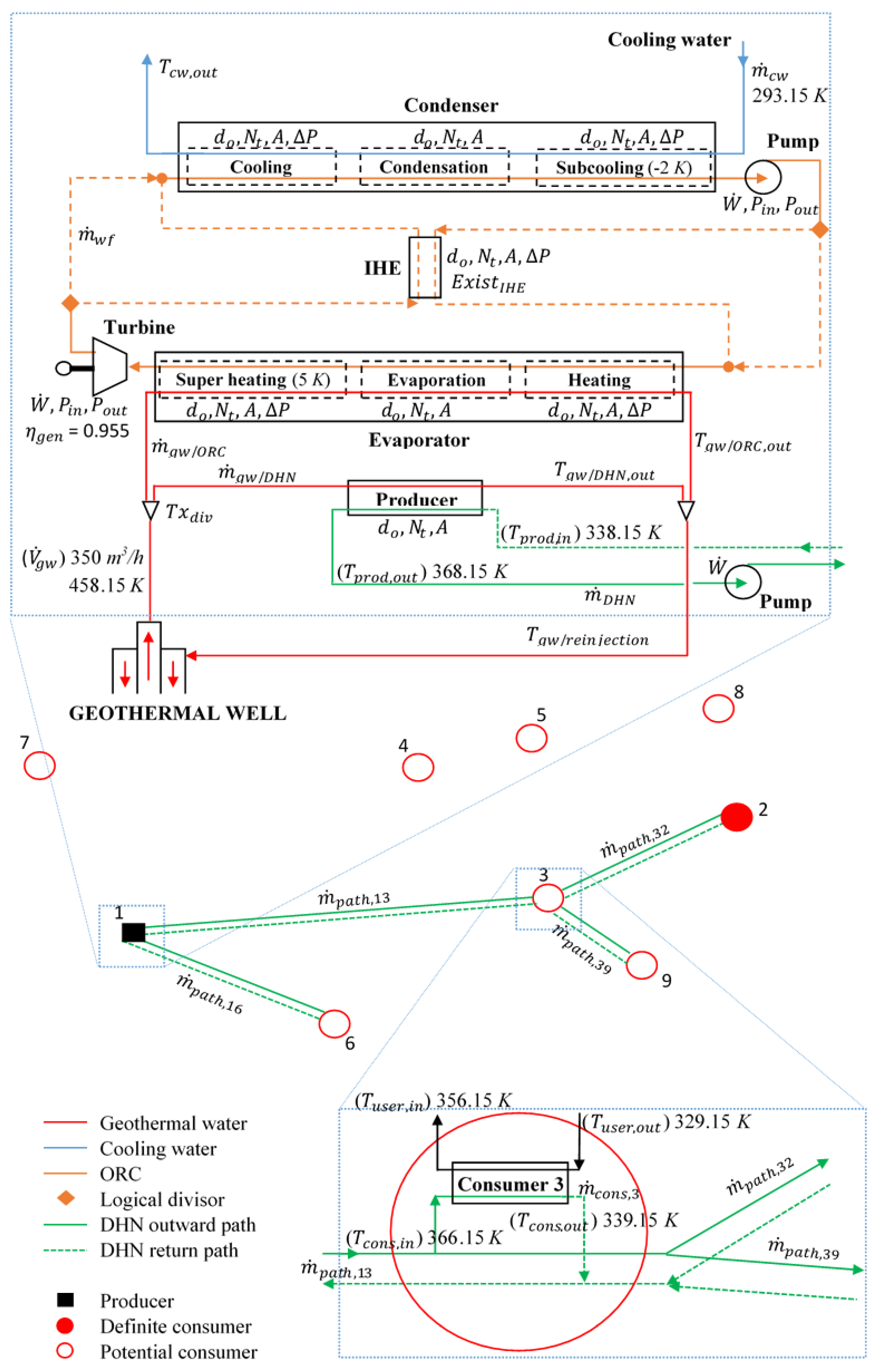
In this energy context, a consortium of ten partners, led by “FONROCHE Géothermie”, is working on the FONGEOSEC project, part of the “Investments for the future” program funded by the French state and managed by the French Agency for Environment and Energy (ADEME). The aim of this project is to design and create an innovative demonstrator of a high-energy geothermal power plant. The geothermal energy will be used to produce electricity and heat. The cycle chosen to produce electricity is an ORC due to its well-known technology and since the nature of the geothermal fluid allows its use. The geothermal fluid also generates heat to supply a District Heating Network (DHN) which is a convenient solution for the heating of buildings, domestic hot water, or industrial applications, for example. A DHN improves energy efficiency compared with individual heat production since it allows great interaction between the different uses which can be cascaded and also the introduction of other renewable energies and industrial waste heat recovery.

Energy and exergy analysis can be used to determine the performance of energy systems. The first one only considers the quantity of energy by application of the first law of thermodynamics. Exergy uses also the second law of thermodynamics and considers irreversibility involved in the system. Exergy represents the quantity and the quality of energy [3]. Comparing energy and exergy analysis for a cogeneration-based district energy system, Rosen et al. [2] have shown that exergy approach provides more useful information than energy analysis and enables to localize accurately inefficient processes. Therefore, for power plants, including geothermal plants, exergy analysis is commonly used to determine the plant performance. Ganjehsarabi et al. [4] carried out an exergy analysis of Dora II geothermal plant based in Turkey. In this plant, cooling towers and turbines were identified as the less performant equipment and responsible for the main part of the exergy destruction (respectively 15% and 12% of total exergy entering the plant), while preheaters were the most performant equipment. The re-injection of the geothermal fluid represented the main exergy losses with 32% of the total exergy input. In this study, the influence of inlet temperature and pressure on exergy performance of turbines was also investigated. A pressure increase led to a negligible performance deterioration, whereas a temperature increase led to a significant performance improvement. Sadreddini et al. [5] performed sensitivity analyses of different parameters on the performance of a Combined Cooling, Heating, and Power plant. The studied parameters were the pinch temperature of heat exchangers, inlet and outlet pressures of the gas turbine, the ORC turbine, the air cavern, and the ejector present in the plant. Since some parameters exhibited reverse influences on exergy performance of the plant, an optimum operating point could be defined. Thereby, the authors presented and highlighted the interest of numerical optimization, which enabled, in their case, a 16.86% decrease in the exergy destruction.

Several studies deal with optimization of an ORC using exergy losses or exergy efficiency, also known as the second law efficiency, as the objective function. Irreversibilities have to be minimized, whereas the exergy efficiency, defined by Equation (1), has to be maximized.

$$\psi =\frac{\dot{E}{x}_{out}}{\dot{E}{x}_{in}}$$

(1)

Depending on choice of $\dot{E}{x}_{in}$ and $\dot{E}{x}_{out}$, different definitions for exergy efficiency can be obtained [3]. In the following literature, authors may not have used the same definition.

In these ORC optimization studies, two aims result in these optimizations:

• The determination of the best working fluid: Dai et al. [6] investigated the ORC performance for low-grade (418.15 K) waste heat recovery. ORC systems with 10 different working fluids were optimized by means of a genetic algorithm. Some parameters are fixed in the same way for the different optimizations (temperature of the condenser, pinch in the evaporator, mass flow rate). Then, turbine inlet temperature and pressure were optimized for each system in order to maximize the exergy efficiency. Isobutane and R-236ea presented the best performance. Roy et al. [7] studied the second law efficiency for three fluids for a similar temperature and more important mass flow of the waste heat source. R-123 had the best results. Second law efficiency was also studied by Heberle et al. [8] for geothermal CHP generation. The parallel and the series connections between the ORC and the heat generation was studied for four fluids in a range of 353–453 K. The most efficient configuration was found to be the series connection using isopentane. For parallel connection, R-227ea gave the best results. Some studies also deal with mixtures as working fluid. Hence, Le et al. [9] studied different mixtures of R-245fa and n-pentane and they obtained that it was the pure n-pentane which exhibited the best performance regarding the maximization of exergetic efficiency. It should be pointed out that in these studies, only thermodynamic considerations have been discussed. Other criteria such as stability, safety, compatibility with material, cost, etc., are not considered.
• The determination of the best configuration: This approach is often coupled with the previous one. For a 453.15 K geothermal source, Yari [10] studied four cycle configurations (simple ORC, ORC with Internal Heat Exchanger (IHE), regenerative ORC, and regenerative ORC with IHE) for three fluids regarding exergy destruction, exergy and energy efficiencies. For exergetic optimization, simple ORC and ORC with IHE presented the same result, which was the best, while regenerative ORC with IHE was better from the energy point of view. Astolfi et al. [11] studied 54 fluids for simple ORC and ORC with IHE. The geothermal source temperature ranged from 393.15 to 453.15 K and superheating of vapor phase was considered. Results confirmed that superheating was non-profitable regarding the second law efficiency and that when the reinjection temperature was limited to 343.15 K, it was worth using an IHE, while simple ORC was preferable when no temperature limit was set. Maraver et al. [12] drew the same conclusion using exergy efficiency optimization for a higher source temperature (573.15 K). However, in their study, for a 443.15 K source the simple ORC had better performance with and without reinjection temperature limit, which is in contradiction with Astolfi et al.’s studies. Then, it appears that the use of the IHE cannot be generalized since its interest depends on the studied case.

For DHN studies, although economic and environmental aspects are widely studied, Rezaie and Rosen [13] confirmed that exergy analysis was a useful tool and provided important information about system performances. Gong and Werner [14] used exergy analysis to compare the four generations of DHN. The use of liquid water instead of steam, from first generation to second generation, and the decrease of the network temperature level up to the fourth generation unsurprisingly led to lower exergy factor (Carnot factor). It can still be reduced in the future using renewables and heat recovery. They also pointed out that currently two thirds of the exergy content in heat supply input are lost in the heat distribution chain and that development of fourth generation DHN should reduce this loss. Sanaei and Nakata [15] optimized the design of a DHN by maximizing exergy efficiency for an existing district. They studied different cases depending on preliminary choice of energy system to recover the heat needed for the DHN. They highlighted that, in some cases, energy efficiencies were very close but these cases could be distinguished by the exergy efficiency. This suggest that exergy is more reliable to evaluate energetic performance of the system.

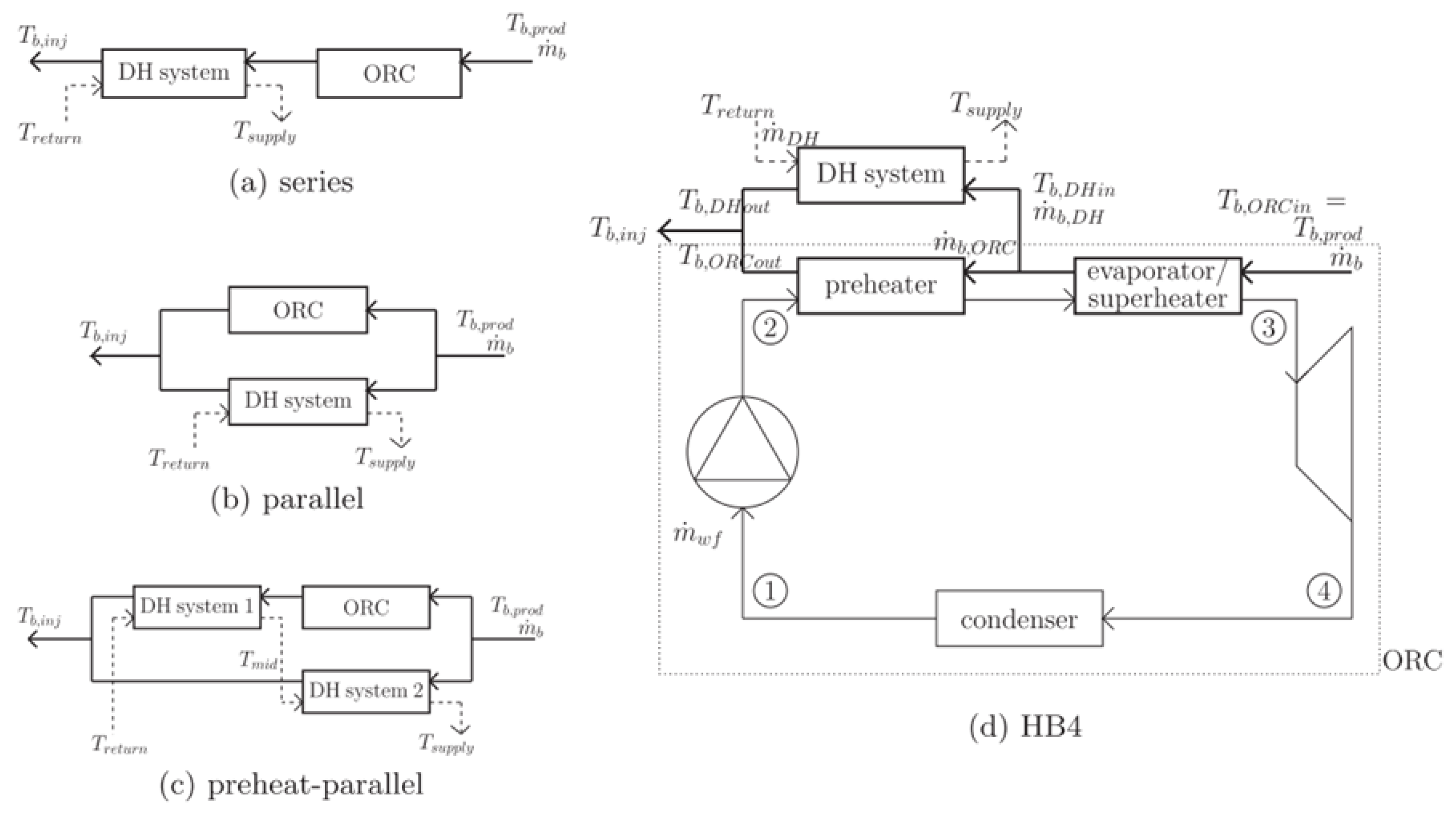
Van Erdeweghe et al. studied the optimal configuration (connection between ORC and DHN) of a geothermal plant. At first, only series and parallel configurations were studied [16]. Next, two other configurations are added: the preheat-parallel and a hybrid (named HB4) configurations [17]. All these configurations are presented in Figure 1. In the HB4 configuration, the evaporation step of the ORC is separated in two parts: an evaporator and a preheater. The geothermal flow rate is split after the evaporator: part of the flow is used in the preheater and part of the flow is used to satisfy the heat demand of the DH system. Hence, the temperature at which the geothermal fluid delivers heat to the DH system is higher compared to the series CHP and lower compared to the parallel CHP. The net power produced was maximized for the four configurations in different conditions (heat demand, supply, and return temperatures for DHN and temperature and mass flow rate of the geothermal source). At the optimal solution, the exergy efficiency was then calculated and configurations were compared. In most cases, the HB4 configuration presented higher efficiency. In case of high-temperature DHN, parallel configuration could exhibit a better performance for low heat demands and low value of geothermal production temperature. However, the exergy efficiency was not optimized and no exergy losses were considered in DHN, which was only represented by heat demand and temperatures. Therefore, the DHN topology was not taken into account. Moreover, among literature on CHP system optimization, simultaneous optimization of the power generation and the heat distribution in CHP plant are not widespread, as specified by Marty et al. [18], who pointed out this need and performed such an optimization.

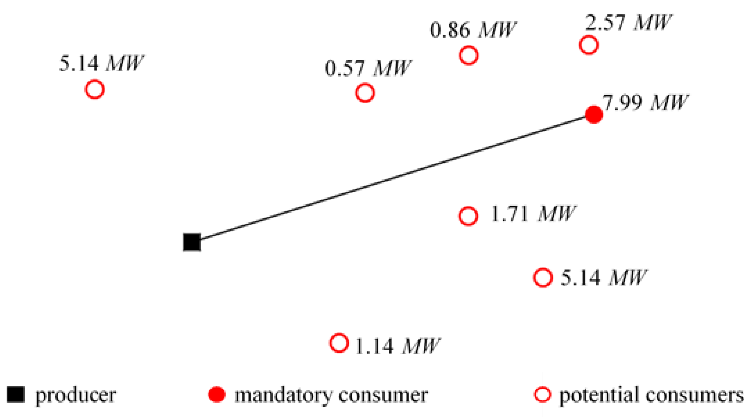
In the present study and the previous one [18], what is original is that the ORC and the DHN topology are simultaneously optimized. A DHN and an ORC system are both supplied in parallel by a geothermal well. The working fluid chosen based on preliminary studies performed by partners, is the R 245fa refrigerant. Only this fluid is considered in the present study. Nevertheless, other fluids will be tested in future studies. The question of the existence of an IHE in the ORC is also considered. Concerning the DHN, the producer is located but its heat production available for the DHN has to be determined based on the consumers’ heat demands. Only one consumer, named definite consumer, is known to be connected to the DHN. Other consumers, named potential consumers, are also considered but their connections to the DHN are not imposed and have to be determined by the optimization. Finally, optimal distribution of the geothermal source for electricity production and for heat production is determined.

The other originality of the present paper is that the studied objective function is now the total exergy loss (including exergy destruction) to be minimizing, whereas the previous paper optimized the annual profit. The optimization problem is first reminded with main assumptions, optimization variables and equations. The exergetic model is then detailed. Exergy analysis is performed for the two optimal solutions (economic and exergetic objective functions), and results are finally compared.

2. CHP Plant Presentation and Formulation of the Optimization Problem

In this part, the optimization problem is described. Apart from the objective function the definition of the optimization problem, assumptions, input data, and optimization variables remain unchanged compared to the economic optimization [18]. They are reminded in the first section. To complete the formulation of the optimization problem, the exergetic model is then described.

2.1. Problem Definition

Solving the optimization problem enables to determine simultaneously:

• temperatures and pressures of the working fluid in the cycle,
• the reinjection temperature of the geothermal water,
• the choice of the use or not of the IHE,
• the sizing of each component of the cycle,
• the distribution of the geothermal source for electricity production and heat production,
• the configuration of the DHN.

In this paper, exergy analysis is performed for two objective functions. $Profit$ is the annual net profit to maximize. $\dot{E}{x}_{loss}$ is the total exergy flow lost (non-used) or destroyed (due to irreversibility in processes) to minimize. Hence, we define two optimization problems described by Equations (2) and (3).

$$\underset{Var,Exist}{\max }Profit\mathrm{s}.\mathrm{t}.Constraints$$

(2)

$$\underset{Var,Exist}{\min }\dot{E}{x}_{loss}\mathrm{s}.\mathrm{t}.Constraints$$

(3)

In each study, the solved system remains the same (variables and equations, which are constraints of the optimization problem). Only the objective function is different $Var$ denotes the set of continuous variables and $Exist$ denotes the set of binary variables.

In order to perform these optimizations, the following assumptions are made:

• The system is considered to be in steady-state condition.
• The geothermal fluid is likened to water.
• The pressure drops throughout pipelines in the ORC are considered to be negligible.
• In the DHN, inlet and outlet temperatures are fixed and are identical for each consumer. This means that the temperatures do not depend on the distance to the producer.

The main variables are presented in the superstructure in Figure 2 and they are:

• The flow rate (${\dot{m}}_{wf}$), the temperatures ($T$) and pressures ($P$) of the working fluid in the cycle, reinjection temperature of the geothermal water and its temperature after its use for the ORC or the DHN ($T_{gw,reinjection}$, $T_{gw/ORC,out}$ and $T_{gw/DHN,out}$), the flow rate (${\dot{m}}_{cw}$), and outlet temperature ($T_{cw,out}$) of the cooling water.
• The variables needed for sizing each equipment of the system. For example, the number of tubes ($N_t$), their diameters ($d_o$) and lengths ($L$), the exchange areas ($A$), the heat transfer coefficients and the pressure drops ($\Delta P$) depending on exchangers.
• The presence or not of the IHE represented by the binary variable $Exis{t}_{IHE}$ which is equal to 1 in case of existence and 0 otherwise.
• The distribution of the use of geothermal water between heat production or electricity production ($T{x}_{div}$).
• The mass flow rate in each canalization between nodes (producer or consumers) (${\dot{m}}_{path,ij}$).

Other variables concern the DHN topology:

• The choice of the connection (or not) to the network of the $i$th consumer ($Exis{t}_i$) and the existence (or not) of the path between two nodes $i$ and $j$ ($Exis{t}_{path,ij}$), which are binary variables. These variables are equal to 1 in case of existence/connection and 0 otherwise. For sake of readability these variables are not represented on Figure 2, but the represented example case corresponds to the following values: only $Exis{t}_1, Exis{t}_2, Exis{t}_3, Exis{t}_6$, and $Exis{t}_9$ are equal to 1 for the connection and $Exis{t}_{path,16}, Exis{t}_{path,13}, Exis{t}_{path,32}$, and $Exis{t}_{path,39}$ for the path.

In Figure 2, each numerical value which is reported is associated with an input data: the temperature and the flow rate of geothermal source, the temperature of the available cooling water and all temperatures in the DHN are input data. In order to avoid condensation in the turbine and cavitation in the pump a 5 K superheating and 2 K subcooling are imposed to the working fluid. Moreover, the efficiency of the electric generator of the turbine (${\eta }_{gen}$) is considered to be equal to 0.955.

The temperature differences of the DHN water for the producer and consumers heat exchangers are chosen to take into account 10% heat losses in the DHN.

Table 1. Heat required (MW) for each consumer.

Consumer	2	3	4	5	6	7	8	9
Heat required (MW)	7.99	1.71	0.57	0.86	1.14	5.14	2.57	5.14

and

Table 2. Distances in km between two nodes (index 1 for the producer, 2 for the definite consumer, 3 to 9 for potential consumers).

$\mathit{i}$$\backslash \mathit{j}$	1	2	3	4	5	6	7	8	9
1		4.46	2.92	2.44	3.56	1.90	1.95	4.70	3.72
2	4.46		1.73	2.43	1.46	3.65	5.27	0.76	1.85
3	2.92	1.73		1.72	1.74	1.93	4.17	2.25	1.04
4	2.44	2.43	1.72		1.17	2.73	2.85	2.42	2.75
5	3.56	1.46	1.74	1.17		3.41	3.97	1.27	2.54
6	1.90	3.65	1.93	2.73	3.41		3.77	4.17	2.26
7	1.95	5.27	4.17	2.85	3.97	3.77		5.23	5.15
8	4.70	0.76	2.25	2.42	1.27	4.17	5.23		2.58
9	3.72	1.85	1.04	2.75	2.54	2.26	5.15	2.58

presented heat required for each consumer and distances between two nodes. Localization of each node is presented in Figure 2. The studied case presents one producer (node 1), one definite consumer (node 2), and seven potential consumers (nodes 3 to 9).

Equations involved in the model of the optimization problem are presented in the next section.

2.2. Equations of the Optimization Problem

2.2.1. Economic Model

The economic model used has been presented in details in previous work [18]. Only the outlines are presented here.

The economic model is based on a physical model for the ORC and the DHN. Mass and energy balances are carried out on each element. Thermodynamic properties of the working fluid in the ORC are estimated using the Peng–Robinson equation of state (EOS) [19] and physical properties for the different fluids are determined by correlations deduced by the U.S. National Institute of Standards and Technology (NIST) online database [20]. The sizing of each element is also carried out. Finally, the economic model estimates the annuity of the total capital investment ($C_{an}$) and the annual working cost ($C_{TPC}$) of the geothermal plant using the sizing. This method was proposed by Turton et al. [21]. The annual profit is then expressed by Equation (4):

$$Profit=\left[1-t{x}_{imp}\right]·\left[S_{elec}+S_{heat}-C_{TPC}-C_{an}\right]$$

(4)

$S_{elec}$ and $S_{heat}$ stand for the annual sale of electricity and heat respectively and $t{x}_{imp}$ stands for the corporate tax rate in France, assumed to be 33.33%.

2.2.2. Exergetic Model

The exergetic model is based on exergy balance on each component. For an open system in steady-state condition, exergy balance presented by Bejan [22] is summarized in Equation (5). In our system, the dead state is characterized by $T_0$ = 20 °C (293.15 K) and $P_0$ = 1 atm (101325 Pa).

$$\dot{E}{x}_Q+{\displaystyle \sum }_{in}{\dot{m}}_{in}·e{x}_{in}=\dot{E}{x}_W+{\displaystyle \sum }_{out}{\dot{m}}_{out}·e{x}_{out}+\dot{E}{x}_d$$

(5)

$in$ and $out$ subscripts refer respectively to inlet and outlet streams. The $ex$ term corresponds to the specific exergy and is expressed by physical specific exergy (thermal, kinetic, and potential) and chemical specific exergy. The kinetic and potential terms are usually neglected [22]. Without chemical reaction or change in composition, $ex$ is expressed by Equation (6):

$$ex=h-h_0-T_0·\left(s-s_0\right)$$

(6)

$h$ and $s$ denote the specific enthalpy and entropy.

The $\dot{E}{x}_W$ term refers to the mechanical exergy flow delivered by the system to its environment and is defined by Equation (7):

$$\dot{E}{x}_W=\dot{W}-P_0\frac{dV}{dt}$$

(7)

For a steady-state system, $P_0\frac{dV}{dt}$ = 0, the mechanical exergy flow is then equal to the mechanical work $\dot{W}$.

The $\dot{E}{x}_Q$ term refers to the thermal exergy flow exchanged with the outlet of the system (counted as positive when the flow enters the system). Except for pipes in the DHN, the system is assumed adiabatic, and this leads to Equation (8):

$$\dot{E}{x}_Q=\left(1-\frac{T_0}{T}\right)·\dot{Q}=0$$

(8)

As shown below, combining Equations (5) to (8), the destroyed exergy flow can be calculated and it is expressed for each component of the system by Equations (9)–(12) and (20)–(23).

• Heat exchangers

  $$\dot{E}{x}_{d,exch}=T_0·\left[{\dot{m}}_h·\left(s_{h,out}-s_{h,in}\right)+{\dot{m}}_c·\left(s_{c,out}-s_{c,in}\right)\right]$$

  (9)
  The subscripts $h$ and $c$ refer respectively to the hot and the cold fluid. For the working fluid of the ORC, specific mass entropy $s$ is estimated by the Peng–Robinson EOS [19]. Liquid water is assumed incompressible, the specific mass entropy difference is estimated by Equation (10):

  $$s_{out}-s_{in}={{\displaystyle \int }}_{T_{in}}^{T_{out}}\frac{C{p}_{l,water}}{T}·dT$$

  (10)
  For the record, the heat capacity $C{p}_{l,water}$ is a function of temperature and is determined by correlations deduced by the NIST online database [20].
• Turbine and ORC pump

  $$\dot{E}{x}_{d,turbine}={\dot{m}}_{wf}·\left[\left(1-{\eta }_{gen}\right)·\left(h_{turbine,in}-h_{turbine,out}\right)-T_0·\left(s_{turbine,in}-s_{turbine,out}\right)\right]$$

  (11)

  $$\dot{E}{x}_{d,ORCpump}={\dot{m}}_{wf}·T_0·\left(s_{ORCpump,out}-s_{ORCpump,in}\right)$$

  (12)
• DHN pump
  The mechanical work supplied to DHN pump must compensate pressure drops. Total pressure drop is the sum of linear (due to frictions) and singular (bends, junctions, exchangers) pressure drops. In this paper, the singular pressure drops are assumed to represent 30% of total pressure drop as proposed by Mertz et al. [23] (Equation (13)).

  $$\Delta P_{tot}=\frac{100}{70}\Delta P_{lin}$$

  (13)
  Where $\Delta P_{lin}$ is determined by the Darcy–Weisbach equation (Equation (14)) where friction coefficient is determined for a turbulent flow by the Blasius correlation (Equation (15)).

  $$\Delta P_{lin}=\frac{\lambda }{d}·\frac{\rho ·v^2}{2}·\left(2·dis{t}_{tot}\right)$$

  (14)

  $$\lambda ={\left[100·Re\right]}^{-0,25}$$

  (15)
  Pipes are not sized in the present study. For the pressure drop determination, it is assumed only one pipe for the whole network circulating the total flow rate ${\dot{m}}_{DHN}$. The pipe diameter $d$ is calculated to meet a water speed $v$ of 1 m/s. The coefficient $2$ is applied to the total length $dis{t}_{tot}$ since two paths of pipe are considered (the outward and the return paths).
  Finally, the mechanical work is expressed by Equation (16).

  $${\dot{W}}_{DHNpump}={\dot{m}}_{DHN}\frac{\Delta P_{tot}}{\rho }$$

  (16)

  Combining Equation (12), applied for DHN pump, and Equation (10), destroyed exergy flow is expressed by Equation (17).

  $$\begin{array}{cc}\hfill \dot{E}{x}_{d,DHNpump}={\dot{m}}_{DHN}·T_0& ·{{\displaystyle \int }}_{T_{DHNpump,in}}^{T_{DHNpump,out}}\frac{C{p}_{l,water}}{T}·dT\hfill \\ \hfill & \approx {\dot{m}}_{DHN}·C{p}_{l,water}·\frac{\left(T_{DHNpump,out}-T_{DHNpump,in}\right)·T_0}{T_{DHNpump,in}}\hfill \end{array}$$

  (17)
  The second part is valid if $T_{DHNpump,out}$ and $T_{DHNpump,in}$ are very close (it is confirmed here since, at the optimal solution, the difference is only 0.05 K). In this condition, relation $\frac{C{p}_{l,water}}{T}$ can be assumed constant. Finally, $\dot{E}{x}_{d,DHNpump}$ can be expressed by Equation (18). ${\dot{W}}_{DHNpump}$ term can be calculated by Equation (16).

  $$\dot{E}{x}_{d,DHNpump}={\dot{W}}_{DHNpump}·\frac{T_0}{T_{DHNpump,in}}$$

  (18)
  Shown on Figure 2, $T_{DHNpump,in}$ is equal to $T_{prod,out}$.
• DHN pipes
  In DHN pipes, the destroyed exergy flow is linked to pressure drops and heat losses and it can be decomposed as proposed on Equation (19):

  $$\dot{E}{x}_{d,pipe}=\dot{E}{x}_{\mathrm{d},\Delta P}+\dot{E}{x}_{d,Q}$$

  (19)
  First, the destroyed exergy linked to pressure drops is due to the work dissipated by friction and is determined by:

  $$\begin{array}{cc}\hfill \dot{E}{x}_{\mathrm{d},\Delta P}={\dot{m}}_{DHN}& \left[h_{DHNpump,out}-h_{DHNpump,in}-T_0·\left(s_{DHNpump,out}-s_{DHNpump,in}\right)\right]\hfill \\ \hfill & \approx {\dot{W}}_{DHNpump}·\left(1-\frac{T_0}{T_{DHNpump,in}}\right)\hfill \end{array}$$

  (20)
  Since the destroyed exergy flow caused by pressure drops is expressed separately, the destroyed exergy flow caused by heat losses is expressed for a constant pressure. Equation (5) then becomes Equation (21):

  $$\dot{E}{x}_{d,Q}=\dot{E}{x}_d-\dot{E}{x}_Q={\displaystyle \sum }_{in}{\dot{m}}_{in}·e{x}_{in}-{\displaystyle \sum }_{out}{\dot{m}}_{out}·e{x}_{out}$$

  (21)
  The $\dot{E}{x}_{d,Q}$ term includes the destroyed exergy flow and the thermal exergy flow lost ($\dot{E}{x}_Q<0$). For outward and return path:

  $$\dot{E}{x}_{d,Q,outward}={\dot{m}}_{DHN}\left[h_{prod,out}-h_{cons,in}-T_0·\left(s_{prod,out}-s_{cons,in}\right)\right]$$

  (22)

  $$\dot{E}{x}_{d,return}={\dot{m}}_{DHN}\left[h_{cons,out}-h_{prod,in}-T_0·\left(s_{cons,out}-s_{prod,in}\right)\right]$$

  (23)

  $$\dot{E}{x}_{d,Q}=\dot{E}{x}_{d,Q,outward}+\dot{E}{x}_{d,return}$$

  (24)
  Entropy differences are determined using the Equation (10) methodology. Enthalpy differences are determined by Equation (25):

  $$h_a-h_b={{\displaystyle \int }}_{T_b}^{T_a}C{p}_{l,water}·dT$$

  (25)
• Other losses
  In addition to the exergy flow destroyed on each component, two exergy flows are non-used and are considered as losses: the outlet exergy flow of the cooling water (Equation (26)) and the exergy flow reinjected in the geothermal well (Equation (27)).

  $$\dot{E}{x}_{cw,out}={\dot{m}}_{cw}\left[h_{cw,out}-h_0-T_0·\left(s_{cw,out}-s_0\right)\right]$$

  (26)

  $$\dot{E}{x}_{reinjection}={\dot{m}}_{gw}\left[h_{reinjection}-h_0-T_0·\left(s_{reinjection}-s_0\right)\right]$$

  (27)

Enthalpy and entropy differences are determined by Equations (10) and (25).

The total exergy flow lost and destroyed is then the sum of the destroyed exergy flow on each component and of the two non-used exergy flows (Equation (28)):

$$\dot{E}{x}_{loss}={\displaystyle \sum }_{component}\dot{E}{x}_{d,component}+\dot{E}{x}_{cw,out}+\dot{E}{x}_{reinjection}$$

(28)

Finally, exergetic performances in the systems are also represented by the exergetic efficiencies. These efficiencies are expressed for each component (heat exchangers, turbine, and pumps) and for each system (ORC, DHN, and the whole plant). Expressions are summarized in

Table 3. Expression of exergy efficiency ($\psi$) for each component and system.

		$\mathit{\psi }$
Components	exchangers	$\frac{\dot{E}{x}_{c,out}-\dot{E}{x}_{c,in}}{\dot{E}{x}_{h,in}-\dot{E}{x}_{h,out}}$
	turbine	$\frac{{\dot{W}}_{turbine}}{\dot{E}{x}_{fluid,in}-\dot{E}{x}_{fluid,out}}$
	pumps	$\frac{\dot{E}{x}_{fluid,out}-\dot{E}{x}_{fluid,in}}{{\dot{W}}_{pump}}$
Systems	ORC	$\frac{{\dot{W}}_{netORC}}{\dot{E}{x}_{gw/ORC,in}}$
	DHN	$\frac{\Delta \dot{E}{x}_{Cons}}{\dot{E}{x}_{gw/DHN,in}}$
	plant	$\frac{{\dot{W}}_{net}+\Delta \dot{E}{x}_{Cons}}{\dot{E}{x}_{gw,in}}=1-\frac{\dot{E}{x}_{loss}}{\dot{E}{x}_{gw,in}}$
For ${\dot{W}}_{netORC}$ only the Organic Rankine Cycle (ORC) pump is considered whereas District Heating Network (DHN) pump is also taken into account in ${\dot{W}}_{net}$.

.

For components, exergy efficiencies are given by Kanoglu [24]. For systems, because reinjection is not revalorized, $\dot{E}{x}_{in}$ term in Equation (1) is considered as the exergy flow rate contained in the geothermal energy source at the production well [25]. $\dot{E}{x}_{out}$ represents the useful exergy at the outlet (${\dot{W}}_{net}={\eta }_{gen}{\dot{W}}_{turbine}-{\dot{W}}_{pumps}$ for electricity production and, because of consumers of the DHN are considered as a closed loop, $\Delta \dot{E}{x}_{cons}=\dot{E}{x}_{cons,out}- \dot{E}{x}_{cons,in}$ for heat production [17]).

2.3. Solution Method

The optimization problem is completed. As discussed in our previous paper [18], the problem presents non-linear equations and integer variables (MINLP problem). The solution strategy detailed in [18] is used to solve the problem and obtain a confident solution. This strategy consists in splitting the general problem into seven steps. Steps are solved successively by increasing the size and the complexity of the problem. The solution of a step is then used as initialization to the next step. This strategy is schematized in Figure 3a, where arrows represent the transfer of previous results as initialization variables. Each optimization sub-problem is represented by a block specifying the objective function and the type of problem (NLP, MINLP). In order to avoid a local solution to the general problem, this one is solved using GAMS^® software tool for 100 random initial conditions as shown in Figure 3b. The confident solution is the best solution obtained, which is expected to be the global solution.

3. Results and Discussions

In this paper, three cases were studied. First, the exergy analysis of the solution of $Profit$ maximization is performed (study denoted $\max Profit$). Secondly, the exergy analysis of the solution of $\dot{E}{x}_{loss}$ minimization with fixed DHN configuration of the solution of the previous study is performed (study denoted $(\min \dot{E}{x}_{loss})$*). Thirdly, the exergy analysis of the solution of $\dot{E}{x}_{loss}$ minimization without constraint on the topology is performed (study denoted $\min \dot{E}{x}_{loss}$). Detail of exergy losses and destruction appearing in the system and exergetic efficiencies are presented in

Table 4. Exergetic efficiency ($\psi$ ) and detail of exergy destroyed and lost for the three different studied cases.

$(\min \dot{E}{x}_{loss})$*: minimization of $\dot{E}{x}_{loss}$ with the DHN structure imposed at the $\max Profit$ solution. Bold values: values appearing on exergy flow diagrams for $\max Profit$ and $\min \dot{E}{x}_{loss}.$ Highlighted values: $\dot{E}{x}_{loss}$ value for the three different optimizations. IHE, Internal Heat Exchanger.

for each studied case. First, it can be noted that none of the optimal design included the IHE.

Finally, a sensitive analysis (impact of temperature and mass flow rate of geothermal source) was performed considering $\dot{E}{x}_{loss}$ minimization.

3.1. Exergy Analysis for $maxProfit$ Solution

At the solution, the exergy flow diagram and the optimal DHN topology obtained in case of $\max Profit$ is presented respectively in Figure 4 and Figure 5. The detail of exergy destructions and losses can be completed with the value presented in Table 4.

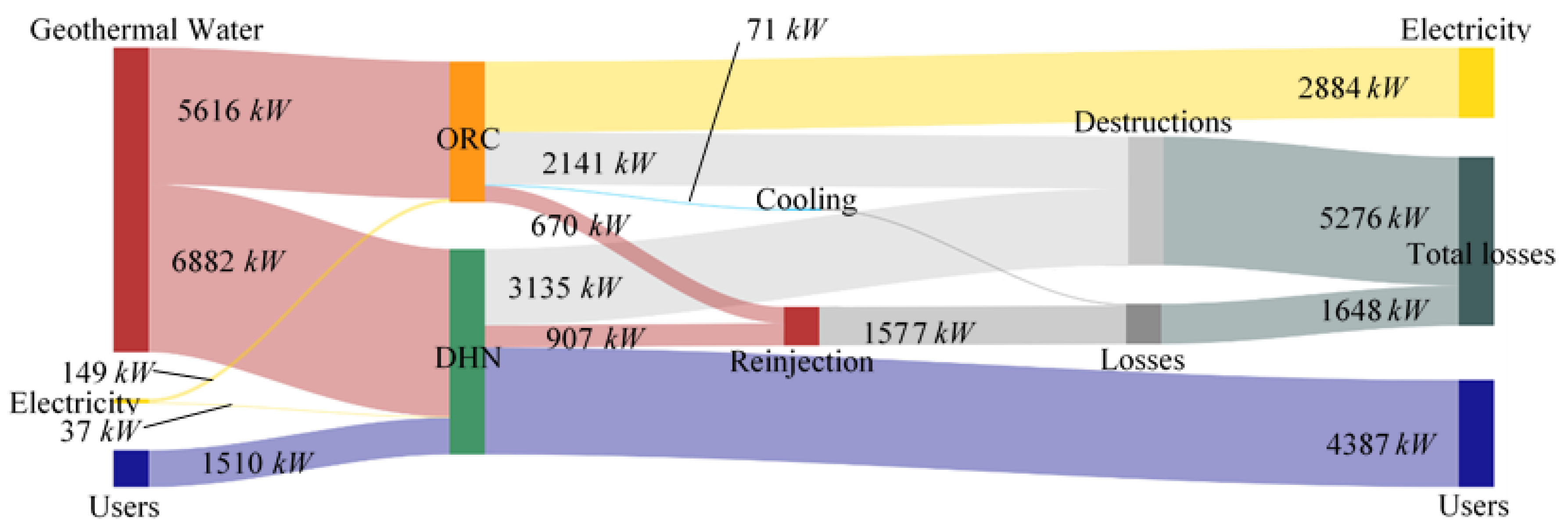
We can see in Figure 4 that destructions represent the main part of total exergy losses (76.2%). Exergy losses induced by the reinjection is widely more important than losses induced by the warming of the cooling water. The main destruction of the system results from the DHN and more specifically from the producer heat exchanger: the exergy destruction in this exchanger represents 70.6% of destructions occurring in the DHN and 32.0% of total exergy losses. In the ORC, evaporator and turbine are responsible for the more exergy destruction (respectively 45.9% and 31.9% of destructions occurring in the ORC and 14.2% and 9.9% of total exergy losses). Nevertheless, the condenser is the less efficient component in the ORC and more generally in the plant. The optimal solution does not involve the IHE in the ORC.

The ORC induces less destruction and losses than the DHN whose exergetic efficiency is slightly lower than the one of the ORC (41.8% against 48.7%).

3.2. Exergy Analysis for $(min\dot{E}{x}_{loss})$* Solution

In this optimization, the DHN configuration is fixed at the configuration of the solution of the previous optimization, which is represented in Figure 5. Since temperature in DHN and heat required are also fixed, the entire DHN is fixed at the previous solution. Only the size of the producer heat exchanger, the geothermal fluid mass flow rate (${\dot{m}}_{gw/DHN}$) and the geothermal outlet temperature ($T_{gw/DHN,out}$) are optimization variables. Then, for this fixed configuration, for a given required heat, a decrease of the temperature of the geothermal source at the outlet of the producer heat exchanger, $T_{gw/DHN,out}$, will lead to a decrease of the mass flow rate, ${\dot{m}}_{gw/DHN}$, and thus an increase of the mass flow rate toward the ORC. This induces an increase of electricity produced and then sold. Moreover, a lower temperature $T_{gw/DHN,out}$ leads to lower losses appearing in reinjection. Then, the two optimizations with the two objective functions ($\max Profit$ and $(\min \dot{E}{x}_{loss})$*) converge toward the same solution regarding the DHN as reported in

Table 5. Values of geothermal water mass flow rate and its temperature at the outlet of DHN and ORC for the three different studied cases.

Systems	Variables	Units	$\mathbf{max}\mathit{P}\mathit{r}\mathit{o}\mathit{f}\mathit{i}\mathit{t}$	$(\mathbf{min}\dot{\mathit{E}}{\mathit{x}}_{\mathit{l}\mathit{o}\mathit{s}\mathit{s}})*$	$\mathbf{min}\dot{\mathit{E}}{\mathit{x}}_{\mathit{l}\mathit{o}\mathit{s}\mathit{s}}$
DHN	${\dot{m}}_{gw/DHN}$	kg·s−1	47.18	47.18	18.87
	$T_{gw/DHN,out}$	K	348.15	348.15	348.15
ORC	${\dot{m}}_{gw/ORC}$	kg·s−1	38.51	38.51	66.82
	$T_{gw/ORC,out}$	K	345.34	344.21	346.14

(which also includes the results for $\min \dot{E}{x}_{loss}$. These results are discussed later). The value of $T_{gw/DHN,out}$ obtained is the lowest as possible, limited by the pinch temperature in the producer.

Regarding the ORC, both objectives converge toward a different $T_{gw/ORC,out}$. This temperature is slightly lower in case of $\left(\min \dot{E}{x}_{loss}\right)$*. Therefore, the losses appearing in reinjection decrease and the heat exchange in evaporator increases. The working fluid mass flow rate, temperatures and pressures are also slightly modified. The destroyed exergy is then increased for the evaporator and the turbine and decreased for the condenser and the pump. Finally, the total losses in the ORC and then in plant is slightly decreased (−0.35% and −0.15% respectively).

3.3. Exergy Analysis for $min\dot{E}{x}_{loss}$ Solution

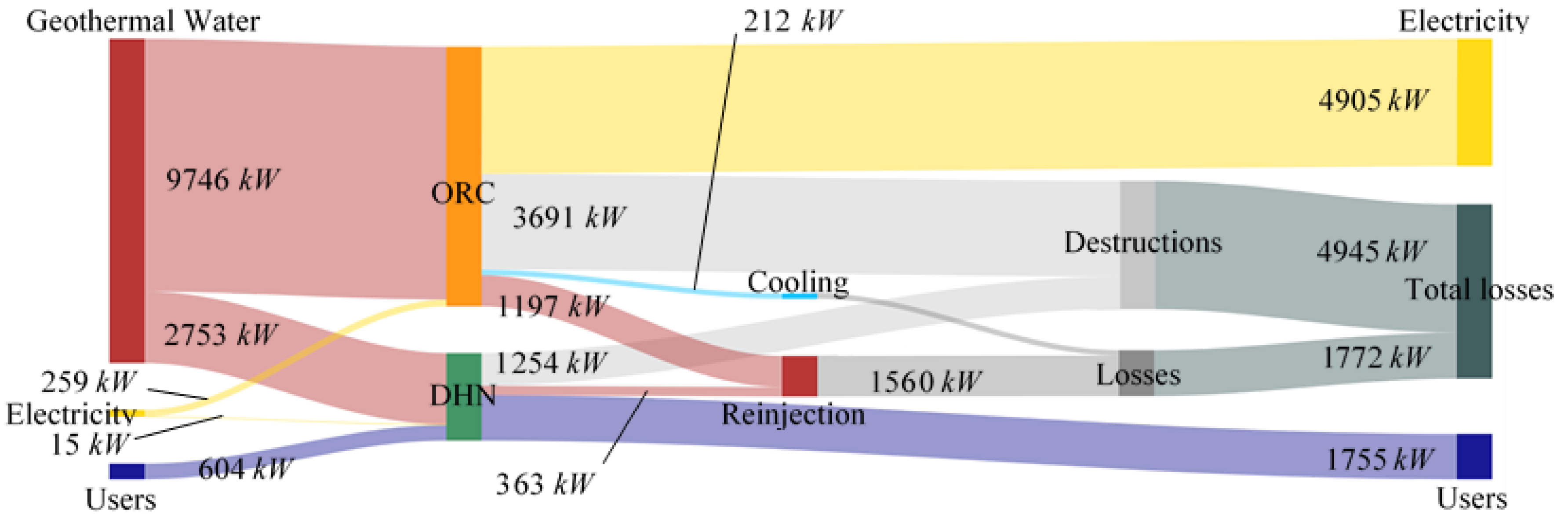
Compared to the previous solution, since the degree of freedom is increased and thus the research field is larger (the DHN configuration is not imposed), a better result is obtained as expected (Table 4). The obtained exergy flow diagram and the optimal DHN topology in case of $\min \dot{E}{x}_{loss}$ are presented respectively in Figure 6 and Figure 7.

The optimal solution is obtained for the smallest as possible DHN (only the definite consumer is connected to the network). Regarding previous results ($\max Profit$ and $(\min \dot{E}{x}_{loss})$* optimizations), the ORC has better efficiency than the DHN. In this solution, this is still true even if ORC efficiency is deteriorated in present case. This could lead to thinking that it is always more interesting, from an exergy point of view, to privilege the ORC as long as ORC exergetic efficiency is the highest. This point is discussed in the next section.

Since DHN temperatures are fixed in the model and optimisations converge toward the same value of $T_{gw/DHN,out}$ (Table 5), exergetic efficiencies for the DHN and its components (pump, producer and consumers heat exchangers) remain unchanged regardless the studied case.

Table 6. Values of $Profit$ and $\dot{E}{x}_{loss}$ for the three different studied cases. For each case, the value of optimized criteria is in bold.

Variables	$\mathbf{max}\mathit{P}\mathit{r}\mathit{o}\mathit{f}\mathit{i}\mathit{t}$	$(\mathbf{min}\dot{\mathit{E}}{\mathit{x}}_{\mathit{l}\mathit{o}\mathit{s}\mathit{s}})*$	$\mathbf{min}\dot{\mathit{E}}{\mathit{x}}_{\mathit{l}\mathit{o}\mathit{s}\mathit{s}}$
$Profit$ (k€/year)	3765	3730	3371
$\dot{E}{x}_{loss}$ (kW)	6924	6913	6717

summarized the value of $Profit$ and $\dot{E}{x}_{loss}$ for the three different studied cases. Regarding exergy losses, the $\min \dot{E}{x}_{loss}$ case enables to decrease the $\dot{E}{x}_{loss}$ value to 207 kW but induces also a decrease to 394 k€/year of $Profit$ (compared to $\max Profit$). A multi-objective approach could enable to find a better compromise to decrease $\dot{E}{x}_{loss}$ without a too important decrease of $Profit$ (not presented in this paper).

Because geothermal water conditions (flow rate and temperature) can be different than the used conditions, a sensitivity analysis on these two conditions was carried out and is presented in the next section.

3.4. Sensitivity Analysis for $min\dot{E}{x}_{loss}$

Evolutions of $\dot{E}{x}_{loss}$, ${\psi }_{ORC}$, ${\psi }_{DHN}$, and ${\psi }_{plant}$ with volumetric flow rate and with the temperature of the inlet geothermal water (respectively ${\dot{V}}_{gw}$ and $T_{gw,in}$) are considered using the $\min \dot{E}{x}_{loss}$ formulation. Each of those parameters are decreased individually. These evolutions are presented in Figure 8 and Figure 9 for the variation of the volumetric flow rate and the variation of the temperature, respectively.

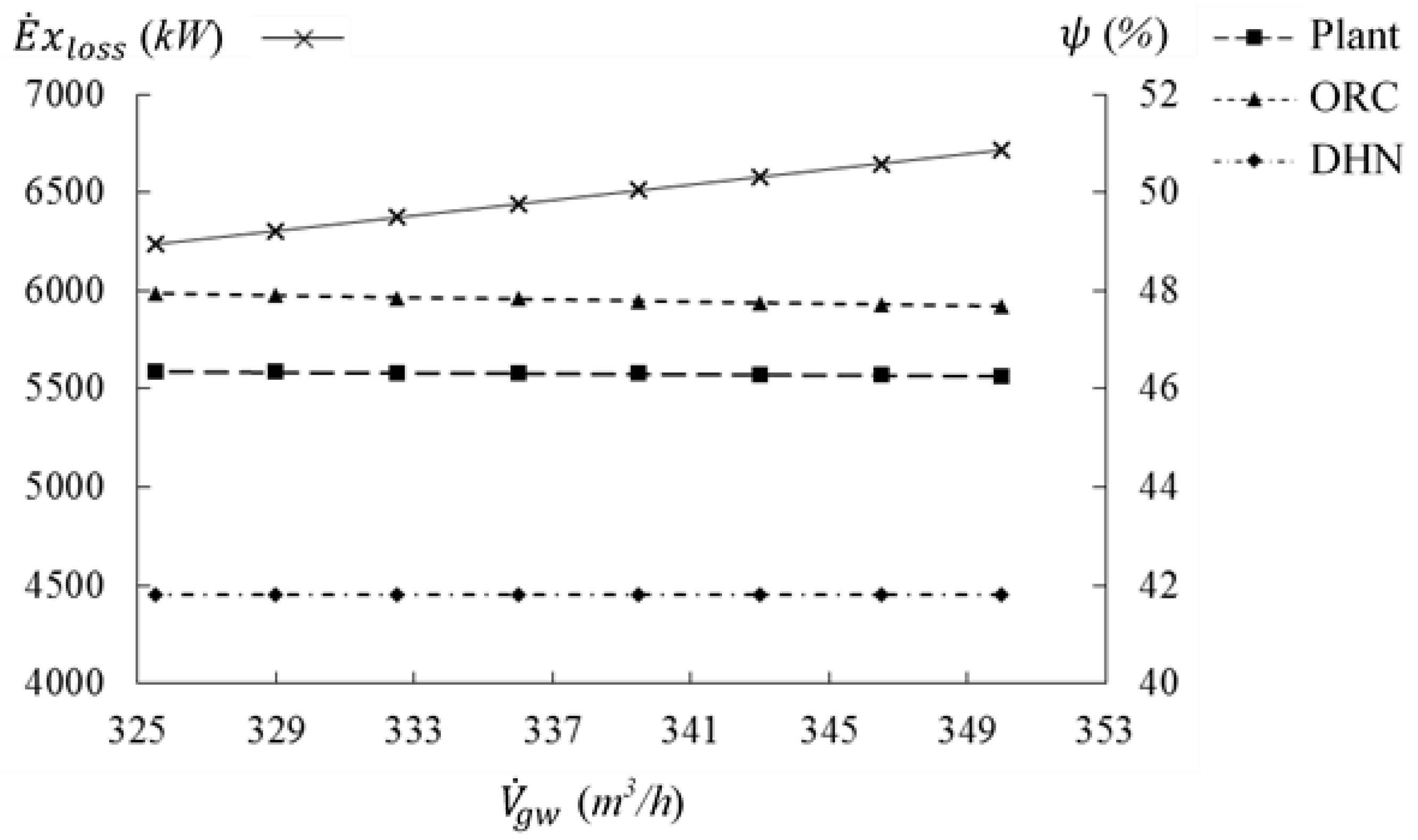
Regarding volumetric flow rate decreasing, the optimal configuration of the DHN remains unchanged (see Figure 7). The flow rate toward the DHN is not modified and efficiency of the DHN is therefore quite similar (Figure 8). The flow rate toward the ORC is necessarily decreased since it is the difference between decreasing geothermal flow rate and constant flow rate toward the DHN. However, the ORC conditions (temperatures and pressures) are nearly the same, then efficiencies of ORC and the plant are slightly increased. A decrease by 7% of volumetric flow rate (transition from 350 m³/h to 325.5 m³/h) leads to a decrease in total exergy losses (−7.15%).

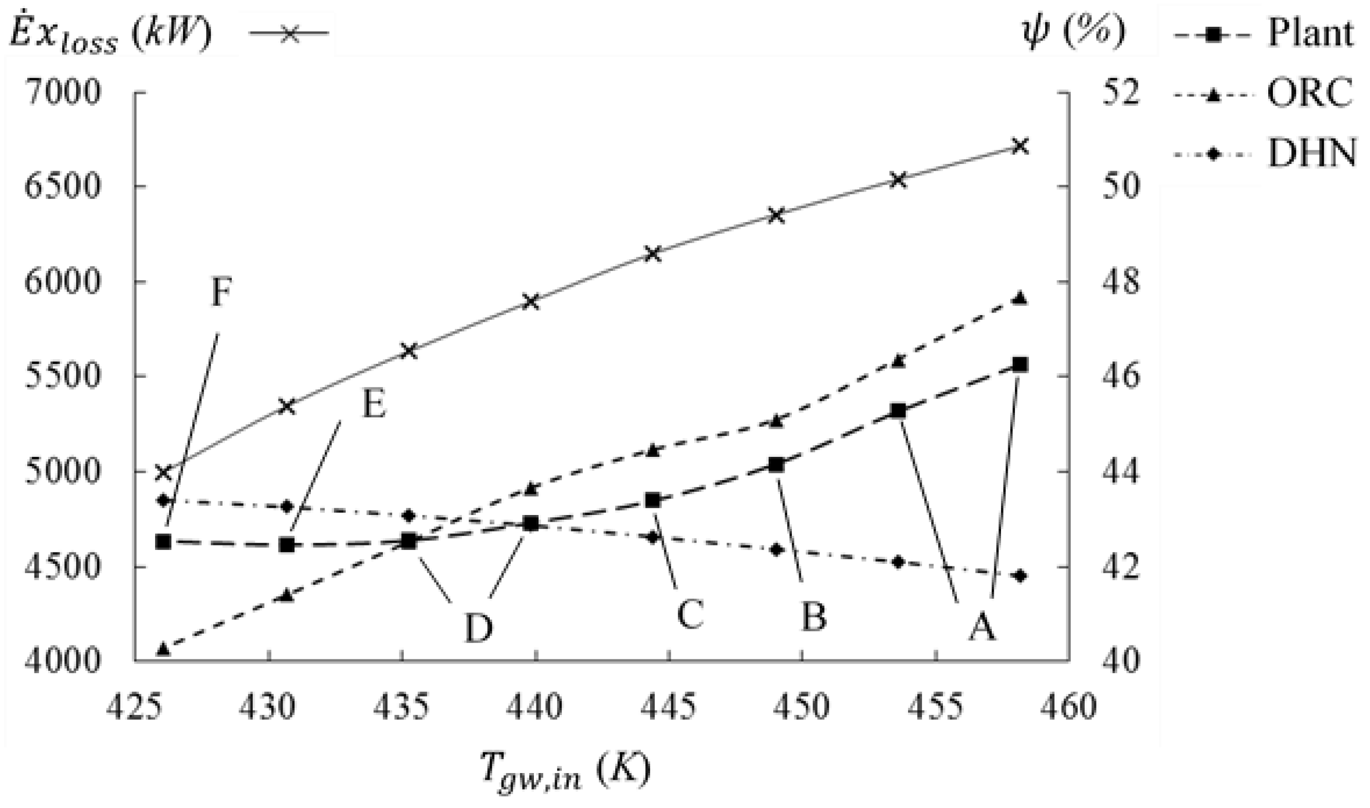
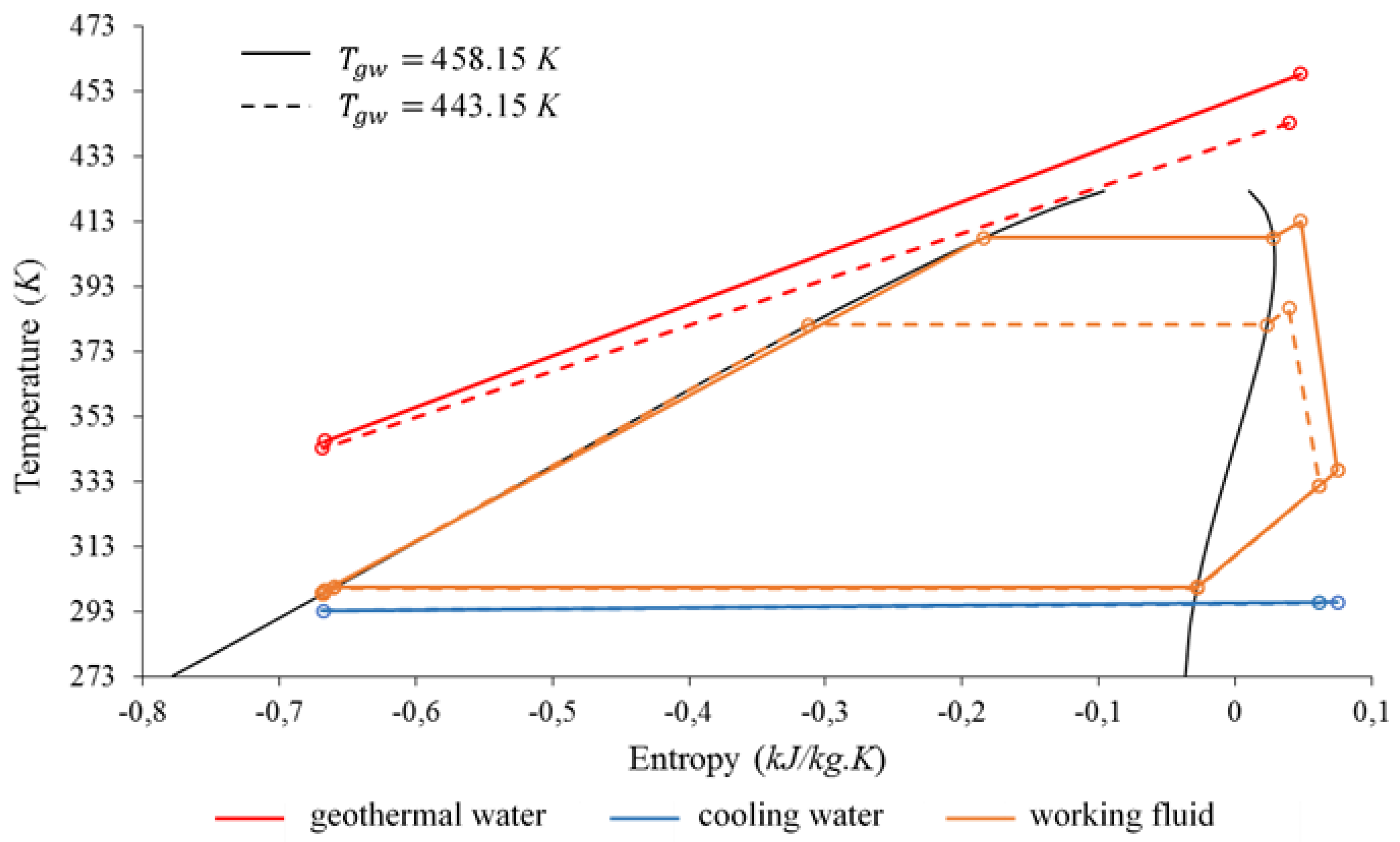
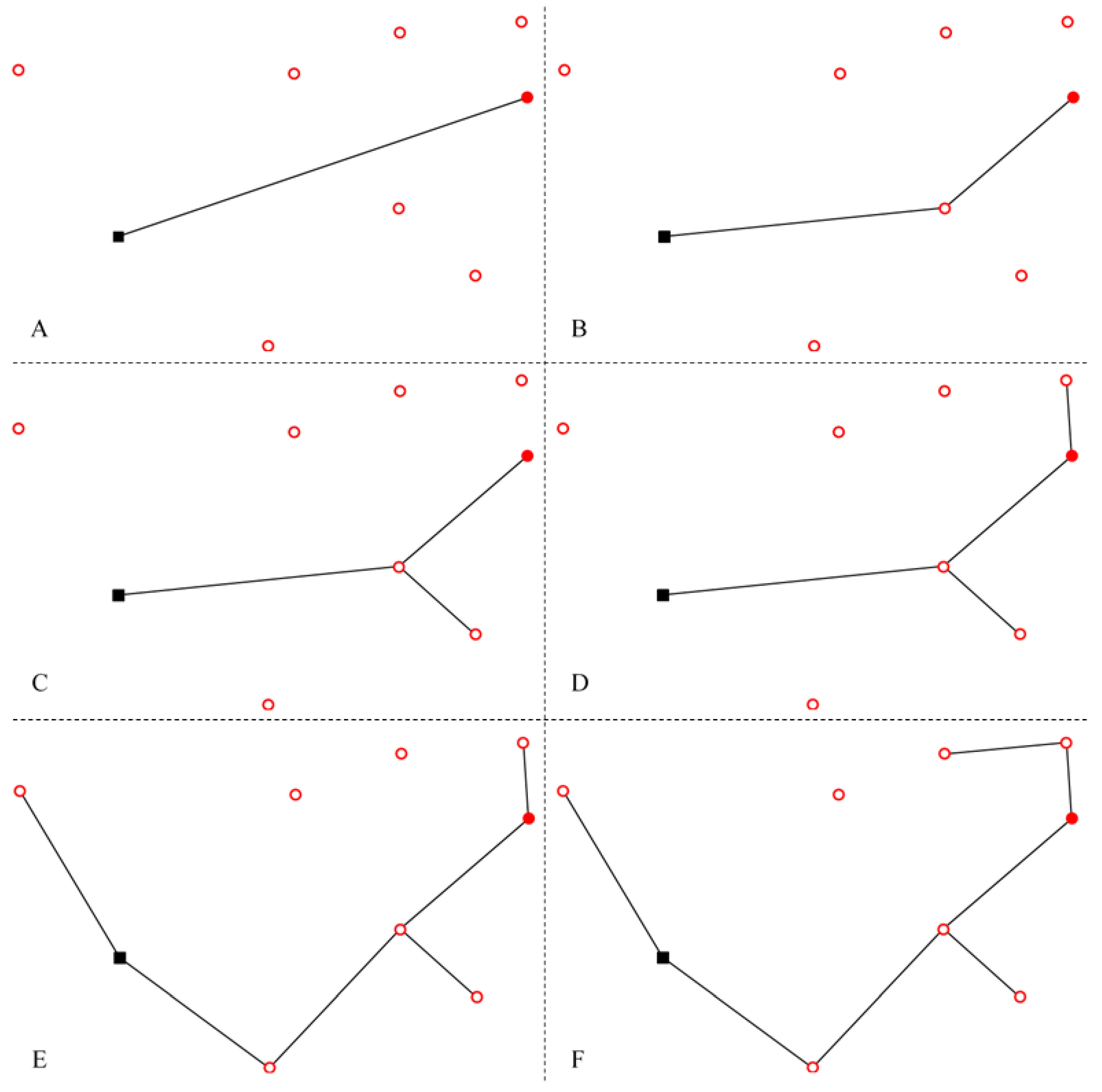
Unlike previous observation on volumetric flow rate decreasing, the decrease of temperature of the geothermal water involves a significant modification of the ORC conditions (easily represented in T-s diagram in Figure 10 already presented in Marty et al. [18]). Figure 9 leads to the conclusion that the lower the temperature, the lower the exergy efficiency of the ORC. Therefore, the flow entering the ORC becomes less important and the flow towards the DHN is more and more privileged. 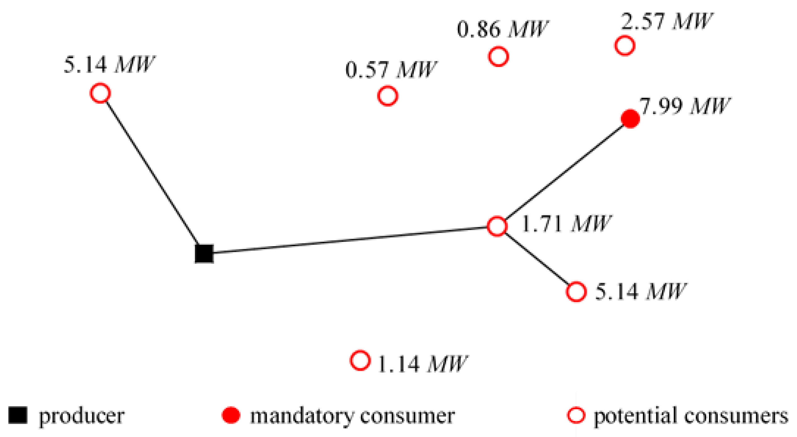In the Figure 9, eight optimization results are presented. These eight results lead to six different DHN configurations denoted from A to F. The corresponding different DHN configurations are presented in Figure 11, which clearly shows that the DHN is increasingly longer as the temperature decreases. In the initial condition ($T_{gw,in}$ = 458.15 K), $T{x}_{div}$ is equal to 22% (22% of geothermal water is used for the DHN). It is equal to 92% for $T_{gw,in}$ = 426.09 K. A temperature decrease by 7% (transition from 458.15 K to 426.09 K) leads to a significant decrease in total exergy losses (−24.90%).

In the previous section, obtaining the possible smallest DHN has led to thinking that this DHN configuration is better as long as the ORC exergetic efficiency is better than that of DHN. The follow-up of the DHN configuration with the geothermal water temperature (especially between about 440 K and 455 K) shows it is not true since B, C, and D configurations (Figure 11) are obtained in this condition. Comparison of exergetic efficiency does not permit concluding about DHN configuration even in case of exergy losses minimization.

4. Conclusions

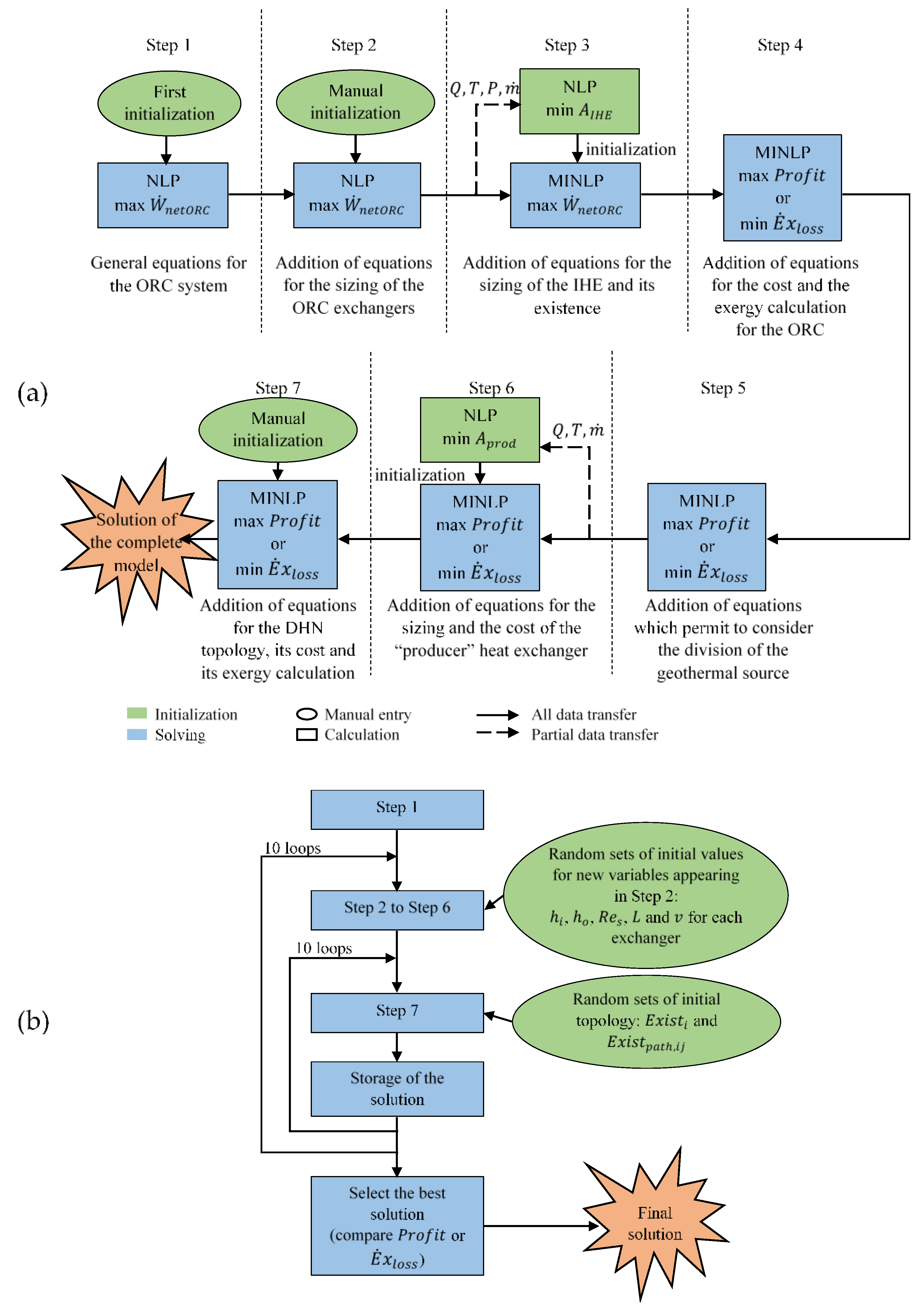
In this paper, an optimization exergy model is presented and applied to a geothermal Combined Heat and Power plant. Setting-up optimization enables to determine simultaneously: (1) the sizing of the Organic Rankine Cycle, (2) the best distribution between electricity and heat production, and (3) the topology of the District Heating Network. In order to solve efficiently the resulting MINLP problem, a solving strategy is used and it has been presented in a previous paper with results of the economic optimization [18]. In the present work, exergetic optimization, using the total exergy losses as objective function is performed.

An exergy analysis is carried out for both optimizations (economic and exergetic). Results show different optimal DHN configurations, the part of the geothermal source toward ORC is then also modified. However, in any cases, evaporator and turbine present the higher exergy destruction in ORC. Although the condenser presents half the exergy destruction of the evaporator, its exergy efficiency is the lowest in the plant. The authors also point out that the minimization of exergy losses tends to lead to a decrease of the DHN size. A sensitivity analysis shows that exergy losses decrease with the decreased of geothermal flow rate and geothermal temperature. The decrease of flow rate does not have significant change on operating points on ORC and DHN configuration. This is not true anymore for the decrease of temperature where operating points on ORC are significantly modified. ORC efficiency drops and the DHN is progressively favoured by the optimization even if ORC efficiency is higher than the DHN one. This reinforces the need to use a simultaneous approach as presented in this work and the previous one [18]. The IHE is never chosen regardless of the studied geothermal conditions. Since DHN temperatures are fixed, DHN and its components efficiencies stay unchanged whatever the studied case. It will be interesting to compare future results (free temperatures) with present results (fixed temperatures) to conclude about influences of this hypothesis. Finally, compared to $\max Profit$, the minimization of $\dot{E}{x}_{loss}$ induces a significant decrease of $Profit$ value. This shows the interest of a future multi-objective study. Indeed, multi-objective optimization can be understood as an efficient way to deal with conflicting objectives simultaneously. There exists a possibly infinite number of solutions among which a trade-off can be chosen to satisfy the preferences of the human decision maker. In the studied case (i.e., the geothermal plant), one can choose to favour economics or exergy savings. In fact, in the past decade, economic optimization was most often favoured regardless of exergy wastes. However, nowadays, to account for the global warming, mentalities and uses have to change. Taking into account exergy efficiency when making a decision will become common. With a multi-objective optimization tool, it will be up to the decision maker to know how far he wants to take it into account. Moreover, the cost of exergy wastes will probably increase, which leads to reducing the gap between the two conflicting objectives.