Optimal Placement of UHF Sensors for Accurate Localization of Partial Discharge Source in GIS


Abstract
:1. Introduction
2. Principle of Method
2.1. Partial Discharge in GIS
2.2. Optimal Placement of UHF Sensors
2.3. Initial PD Location Method
2.4. Accurate PD Location Method for GIS
- 1)
- Acquire the EM wave arriving time matrix TM = [T1T2T3…TP]T and the corresponding node matrix S = [S1S2S3…SP] from UHF sensors after PD occurs.
- 2)
- Based on Sm corresponding to Tmin, w × (P – 1) PD location combinations are composed of w adjacent nodes and P – 1 UHF sensors.
- 3)
- The initial PD position can be calculated by the measure matrix E, and the occurring time t0 of PD can be found.
- 4)
- Combining t0 with the topology structure of GIS, the PD position can be revised by multiple sensors of the GIS to obtain the accurate PD location results.
2.5. Noise Reduction Method
- 1)
- Determine the number of decomposition layers of DTCWT. Different layers will affect the accuracy and speed of noise reduction calculation.
- 2)
- Decompose the noisy signal by DTCWT. The signal is transformed by n-layer dual-tree complex wavelet transform. The inverse transform of the wavelet coefficients of layer i is implemented to obtain the wavelet components of layer i. A matrix can be formed by signal components at different scales of signal transformation:
- 3)
- Screen Signal Components. The time kurtosis of signal Di can be found:The envelope spectral kurtosis can be found:where HT is Hilbert transform. The higher time kurtosis and envelope spectral kurtosis indicate that there are more partial discharge impulse components in Di. The product of time domain kurtosis and envelope spectral kurtosis (index TE) of each component is calculated, and the component with large product is selected for reconstruction.
- 4)
- The selected DTCWT detail signal component is processed by MKD denoising, and then the inverse DTCWT transform is used to reconstruct the signal. After the inverse transform, the denoised signal of the component can be obtained.
3. Experimental Results and Analysis
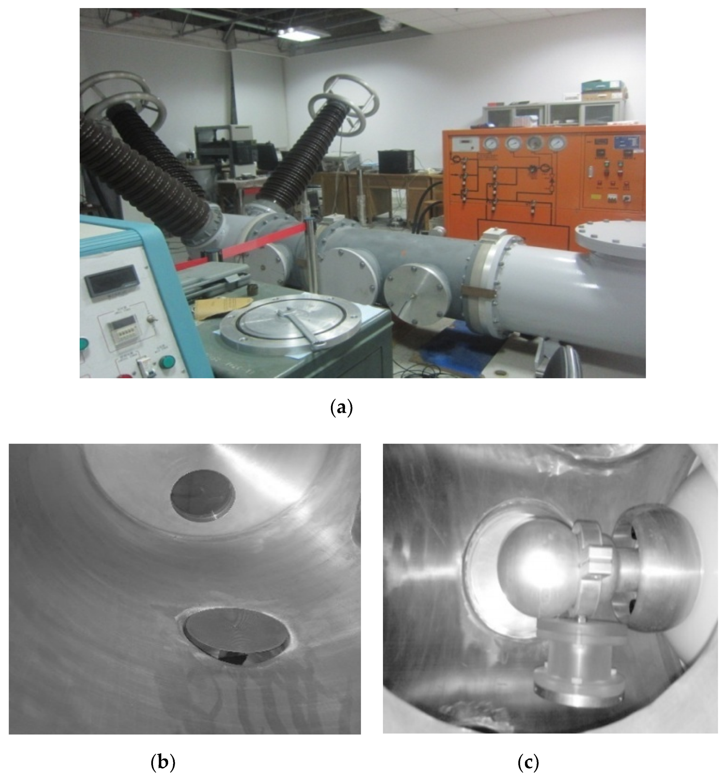
3.1. Experimental Platform
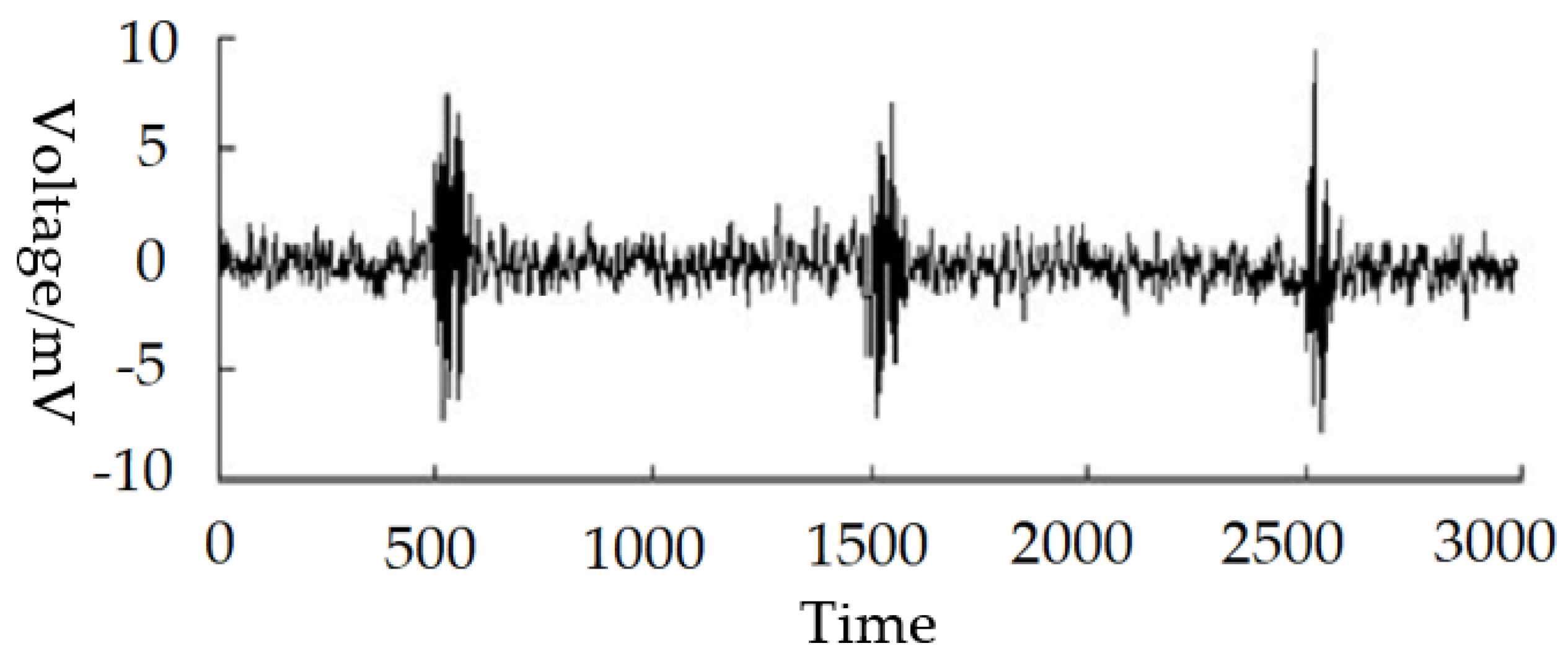
3.2. Noise Reduction
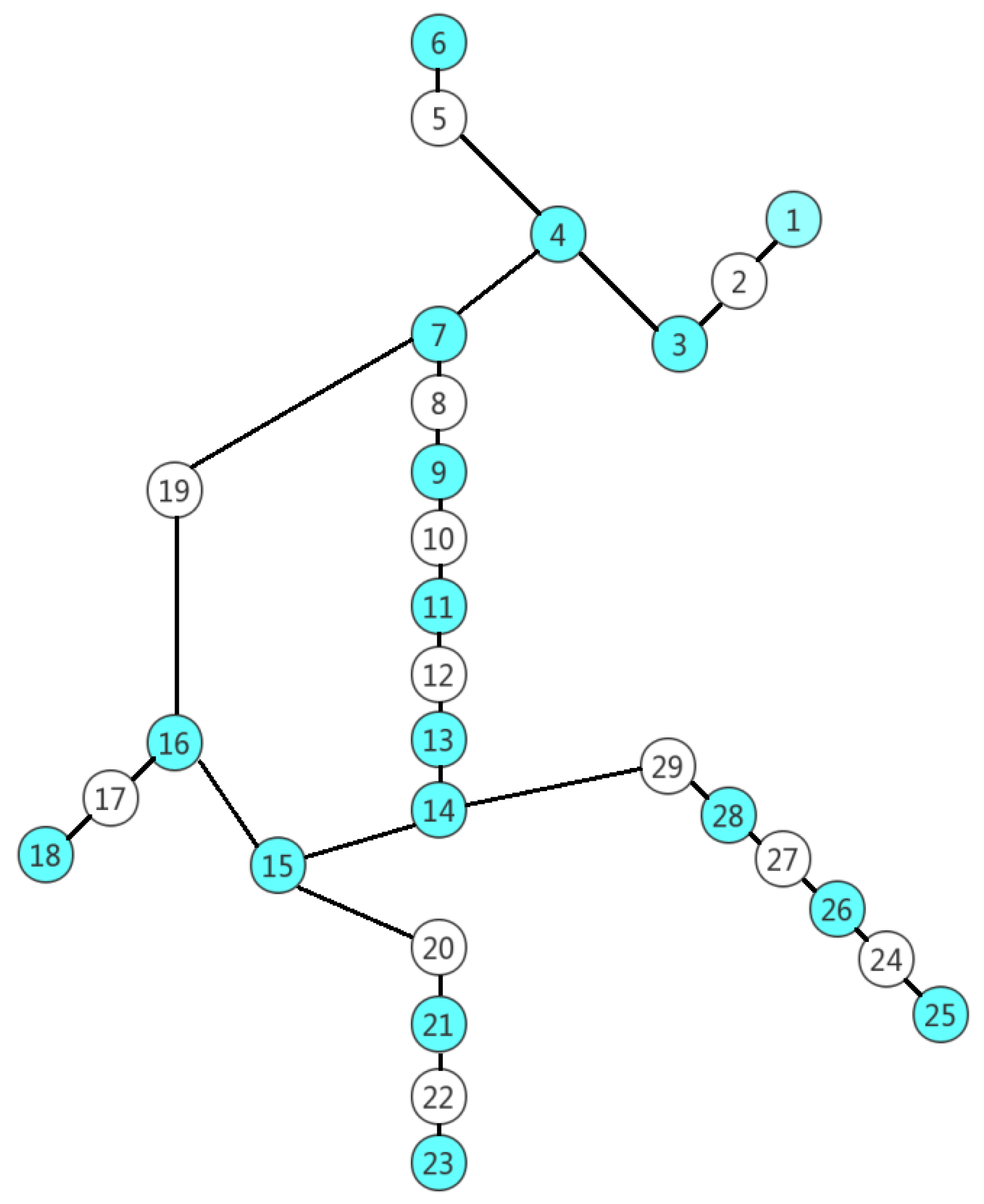
3.3. Optimal Placement
3.4. PD Location Results
3.5. Fault Tolerance Analysis
3.6. Comparison of Methods
4. Conclusions
Author Contributions
Funding
Conflicts of Interest
References
- Si, W.R.; Li, J.H.; Li, D.J.; Yang, J.G.; Li, Y.M. Investigation of a Comprehensive Identification Method Used in Acoustic Detection System for GIS. IEEE Trans. Dielectr. Electr. Insul. 2010, 17, 721–732. [Google Scholar] [CrossRef]
- OKabe, S.; Yamagiwa, T.; Okubo, H. Detection of Harmful Metallic Particles Inside Gas Insulated Switchgear using UHF Sensor. IEEE Trans. Dielectr. Electr. Insul. 2008, 15, 701–709. [Google Scholar] [CrossRef]
- OKabe, S.; Ueta, G.; Hama, H.; Ito, T.; Hikita, M.; Okubo, H. New aspects of UHF PD diagnostics on gas-insulated systems. IEEE Trans. Dielectr. Electr. Insul. 2014, 21, 2245–2258. [Google Scholar] [CrossRef]
- Mirzaei, H.R.; Akbari, A.; Gockenbach, E.; Miralikhani, K. Advancing new techniques for UHF PD detection and localization in the power transformers in the factory tests. IEEE Trans. Dielectr. Electr. Insul. 2015, 22, 448–455. [Google Scholar] [CrossRef]
- Ishak, A.M.; Ishak, M.T.; Jusoh, M.T.; Dardin Syed, S.F.; Judd, M.D. Design and optimazation of UHF partial discharge sensors using FDTD modeling. IEEE Sens. J. 2017, 17, 127–133. [Google Scholar]
- Wang, Y.; Wang, X.; Li, J. UHF moore fractal antennas for online GIS PD detection. IEEE Antennas Wirel. Propag. Lett. 2017, 16, 852–855. [Google Scholar] [CrossRef]
- Tenbohlen, S.; Denissov, D.; Hoek, S.M.; Markalous, S.M. Partial discharge measurement in the ultra-high frequency (UHF) range. IEEE Trans. Dielectr. Electr. Insul. 2008, 15, 1544–1552. [Google Scholar] [CrossRef]
- Xu, Y.; Liu, W.; Gao, W. Investigation of disc-type sensors using the UHF method to detect partial discharge in GIS. IEEE Trans. Dielectr. Electr. Insul. 2015, 22, 3019–3027. [Google Scholar] [CrossRef]
- Sinaga, H.H.; Phung, B.T.; Blackburn, T.R. Recognition of single and multiple partial discharge sources in transformers based on ultra-high frequency signals. IET Gener. Transm. Distrib. 2014, 8, 160–169. [Google Scholar] [CrossRef]
- Boya, C.; Rojas, M.V.; Ruiz, M.; Robles, G. Location of partial discharges sources by means of blind source separation of UHF signals. IEEE Trans. Dielectr. Electr. Insul. 2015, 22, 2302–2310. [Google Scholar] [CrossRef]
- Gao, W.; Ding, D.; Liu, W. Research on the typical partial discharge using the UHF detection method for GIS. IEEE Trans. Power Deliv. 2011, 26, 2621–2629. [Google Scholar] [CrossRef]
- Zhang, G.B.; Guo, J.B.; Chu, F.H.; Zhang, Y.C. Environmental-adaptive indoor radio path loss model for wireless sensor networks localization. Int. J. Electron. Commun. 2011, 65, 1023–1031. [Google Scholar] [CrossRef]
- Iorkyase, E.T.; Tachtatzis, C.; Atkinson, R.C.; Glover, I.A. Localization of partial discharge sources using radio fingerprinting technique. In Proceedings of the 2015 Loughborough Antennas & Propagation Conference (LAPC), Loughborough, UK, 2–3 November 2015; pp. 1–5. [Google Scholar]
- Ito, T.; Kamei, M.; Ueta, G.; Okabe, S. Improving the sensitivity verification method of the UHF PD detection technique for GIS. IEEE Trans. Dielectr. Electr. Insul. 2012, 18, 1847–1853. [Google Scholar] [CrossRef]
- Reid, A.J.; Judd, M.D.; Fouracre, R.A.; Stewart, B.; Hepburn, D.M. Simultaneous measurement of partial discharges using IEC60270 and radio-frequency techniques. IEEE Trans. Dielectr. Electr. Insul. 2011, 18, 444–455. [Google Scholar] [CrossRef]
- Zheng, S.; Li, C.; Tang, Z.; Chang, W.; He, M. Location of PDs inside transformer windings using UHF methods. IEEE Trans. Dielectr. Electr. Insul. 2014, 21, 386–393. [Google Scholar] [CrossRef]
- Hekmati, A.; Hekmati, R. Optimum acoustic sensor placement for partial discharge allocation in transformers. IET Sci. Meas. Technol. 2017, 11, 581–589. [Google Scholar] [CrossRef]
- Dai, D.; Wang, X.; Long, J.; Tian, M.; Zhu, G.; Zhang, J. Feature extraction of GIS partial discharge signal based on S-transform and singular value decomposition. IET Sci. Meas. Technol. 2017, 11, 186–193. [Google Scholar] [CrossRef]
- Gao, W.; Ding, D.; Liu, W.; Huang, X. Propagation attenuation properties of partial discharge in typical in-field GIS structures. IEEE Trans. Power Deliv. 2013, 28, 2540–2549. [Google Scholar] [CrossRef]
- Hikita, M.; Ohtsuka, S.; Wada, J.; Okabe, S.; Hoshino, T.; Maruyama, S. Propagation properties of PD-induced electromagnetic wave in 66 kV GIS model tank with L branch structure. IEEE Trans. Dielectr. Electr. Insul. 2011, 18, 1678–1685. [Google Scholar] [CrossRef]
- Hikita, M.; Ohtsuka, S.; Ueta, G.; Okabe, S.; Hoshino, T.; Maruyama, S. Influence of insulating spacer type on propagation properties of PD-induced electromagnetic wave in GIS. IEEE Trans. Dielectr. Electr. Insul. 2010, 17, 1642–1648. [Google Scholar] [CrossRef]
- Li, T.; Wang, X.; Zheng, C.; Liu, D.; Rong, M. Investigation on the placement effect of UHF sensor and propagation characteristics of PD-induced electromagnetic wave in GIS based on FDTD method. IEEE Trans. Dielectr. Electr. Insul. 2014, 21, 1015–1025. [Google Scholar] [CrossRef]
- Li, X.; Wang, X.; Yang, A.; Xie, D.; Ding, D.; Rong, M. Propogation characteristics of PD-induced UHF signal in 126 kV GIS with three-phase construction based on time-frequency analysis. IET Sci. Meas. Technol. 2016, 10, 805–812. [Google Scholar] [CrossRef]
- Markalous, S.M.; Tenbohlen, S.; Feser, K. Detection and location of partial discharges in power transformers using acoustic and electromagnetic signals. IEEE Trans. Dielectr. Electr. Insul. 2008, 15, 1576–1583. [Google Scholar] [CrossRef]
- Tang, J.; Xie, Y. Partial discharge location based on time difference of energy accumulation curve of multiple signals. IET Electr. Power Appl. 2011, 5, 175–180. [Google Scholar] [CrossRef]
- Zhang, Q.; Li, C.; Zheng, S.; Yin, H.; Kan, Y.; Xiong, J. Remote detecting and locating partial discharge in bushings by using wideband RF antenna array. IEEE Trans. Dielectr. Electr. Insul. 2016, 23, 3575–3583. [Google Scholar] [CrossRef]
- Liang, R.; Xu, C.; Wang, F.; Cheng, Z.; Shen, X. Optimal deployment of fault location devices based on wide area travelling wave information in complex power grid. Trans. China Electrotech. Soc. 2016, 31, 30–38. [Google Scholar]
- Le, Q.; Zhen, Z.; Pei, Y. Image identification of insects based on color histogram and dual tree complex wavelet transform (DTCWT). Acta Entomol. Sin. 2010, 53, 91–97. [Google Scholar]
- Zhang, W.; Bi, K.; Luo, L.; Sheng, G.; Jiang, X. RSSI fingerprinting-based UHF partial discharge localization technology. In Proceedings of the Power & Energy Engineering Conference, Xi’an, China, 25–28 October 2016; pp. 1364–1367. [Google Scholar]
- Li, Z.; Luo, L.G.; Sheng, G.H.; Liu, Y.; Jiang, X. UHF partial discharge localisation method in substation based on dimension-reduced RSSI fingerprint. IET Gener. Transm. Distrib. 2018, 12, 398–405. [Google Scholar] [CrossRef]


| DTCWT | Improved DTCWT | |
|---|---|---|
| SNR | 7.59 | 20.07 |
| VTP | 1.495 | 1.030 |
| Section | Length (mm) | Section | Length (mm) |
|---|---|---|---|
| 1–2 | 3826 | 16–17 | 1060 |
| 2–3 | 1705 | 17–18 | 3413 |
| 3–4 | 1153 | 16–19 | 1715 |
| 4–5 | 2494 | 19–7 | 3380 |
| 5–6 | 1155 | 15–20 | 1035 |
| 4–7 | 1550 | 20–21 | 1380 |
| 7–8 | 1133 | 21–22 | 2860 |
| 8–9 | 3485 | 22–23 | 1380 |
| 9–10 | 2550 | 23–24 | 1060 |
| 10–11 | 8210 | 24–25 | 1250 |
| 11–12 | 2550 | 24–26 | 3460 |
| 12–13 | 3485 | 26–27 | 990 |
| 13–14 | 1740 | 27–28 | 990 |
| 14–15 | 3380 | 28–29 | 3790 |
| 15–16 | 1715 | 29–14 | 1740 |
| Sensor Number | Time (ns) | Sensor Number | Time (ns) |
|---|---|---|---|
| 1 | 34.7 | 15 | 29.3 |
| 3 | 15.7 | 16 | 24.3 |
| 4 | 12.6 | 18 | 39.4 |
| 6 | 24.3 | 21 | 37.3 |
| 7 | 7.3 | 23 | 52.5 |
| 9 | 7.9 | 25 | 59.4 |
| 11 | 43.8 | 26 | 66.6 |
| 13 | 47.2 | 28 | 59.1 |
| 14 | 40.5 | -- | -- |
| Sensor Combination | Euclidean Distance | PD Section | PD Position (mm) |
|---|---|---|---|
| (1,7) | 8.9 | 3‒4 | 7.0 × 10⁻² |
| (3,7) | 6.8 | 4‒7 | 1.2 × 10⁻¹ |
| (4,7) | 7.0 | 4‒7 | 2.4 × 10⁻¹ |
| (6,7) | 8.8 | 5‒6 | 1.2 |
| (9,7) | 1.9 | 8‒9 | 915.0 |
| (11,7) | 0.8 | 8‒9 | 954.3 |
| (13,7) | 2.3 | 8‒9 | 1113.4 |
| (14,7) | 1.9 | 8‒9 | 903.5 |
| (15,7) | 1.7 | 8‒9 | 954.3 |
| (16,7) | 1.8 | 8‒9 | 915.0 |
| (18,7) | 3.9 | 4‒5 | 1.3 × 10⁻³ |
| (21,7) | 1.7 | 8‒9 | 923.5 |
| (23,7) | 2.1 | 8‒9 | 903.5 |
| (25,7) | 1.2 | 8‒9 | 1078.2 |
| (26,7) | 1.9 | 8‒9 | 915.0 |
| (28,7) | 1.8 | 8‒9 | 1093.4 |
| Sensor Number | PD Position (mm) | Absolute Error (mm) |
|---|---|---|
| 1 | 1098.4 | 98.4 |
| 3 | 1123.9 | 123.9 |
| 4 | 1087.0 | 87.0 |
| 6 | 923.5 | 76.5 |
| 7 | 883.5 | 116.5 |
| 9 | 1095.8 | 95.8 |
| 11 | 913.9 | 86.1 |
| 13 | 913.4 | 86.5 |
| 14 | 954.3 | 45.7 |
| 15 | 902.7 | 97.3 |
| 16 | 906.6 | 93.4 |
| 18 | 1087.9 | 87.9 |
| 21 | 1077.2 | 77.2 |
| 23 | 923.5 | 76.5 |
| 25 | 893.7 | 106.3 |
| 26 | 914.2 | 85.8 |
| 28 | 1092.6 | 92.6 |
| Proposed Method | RSSI | |
|---|---|---|
| average absolute error (mm) | 22.8 | 107.7 |
| absolute error < 50 mm (%) | 100 | 50 |
| absolute error < 100 mm (%) | 100 | 66.7 |
| absolute error < 200 mm (%) | 100 | 83.3 |
| Maximum absolute error (mm) | 42.3 | 238.5 |
© 2019 by the authors. Licensee MDPI, Basel, Switzerland. This article is an open access article distributed under the terms and conditions of the Creative Commons Attribution (CC BY) license (http://creativecommons.org/licenses/by/4.0/).
Share and Cite
Liang, R.; Wu, S.; Chi, P.; Peng, N.; Li, Y. Optimal Placement of UHF Sensors for Accurate Localization of Partial Discharge Source in GIS. Energies 2019, 12, 1173. https://doi.org/10.3390/en12061173
Liang R, Wu S, Chi P, Peng N, Li Y. Optimal Placement of UHF Sensors for Accurate Localization of Partial Discharge Source in GIS. Energies. 2019; 12(6):1173. https://doi.org/10.3390/en12061173
Chicago/Turabian StyleLiang, Rui, Shenglei Wu, Peng Chi, Nan Peng, and Yi Li. 2019. "Optimal Placement of UHF Sensors for Accurate Localization of Partial Discharge Source in GIS" Energies 12, no. 6: 1173. https://doi.org/10.3390/en12061173
APA StyleLiang, R., Wu, S., Chi, P., Peng, N., & Li, Y. (2019). Optimal Placement of UHF Sensors for Accurate Localization of Partial Discharge Source in GIS. Energies, 12(6), 1173. https://doi.org/10.3390/en12061173