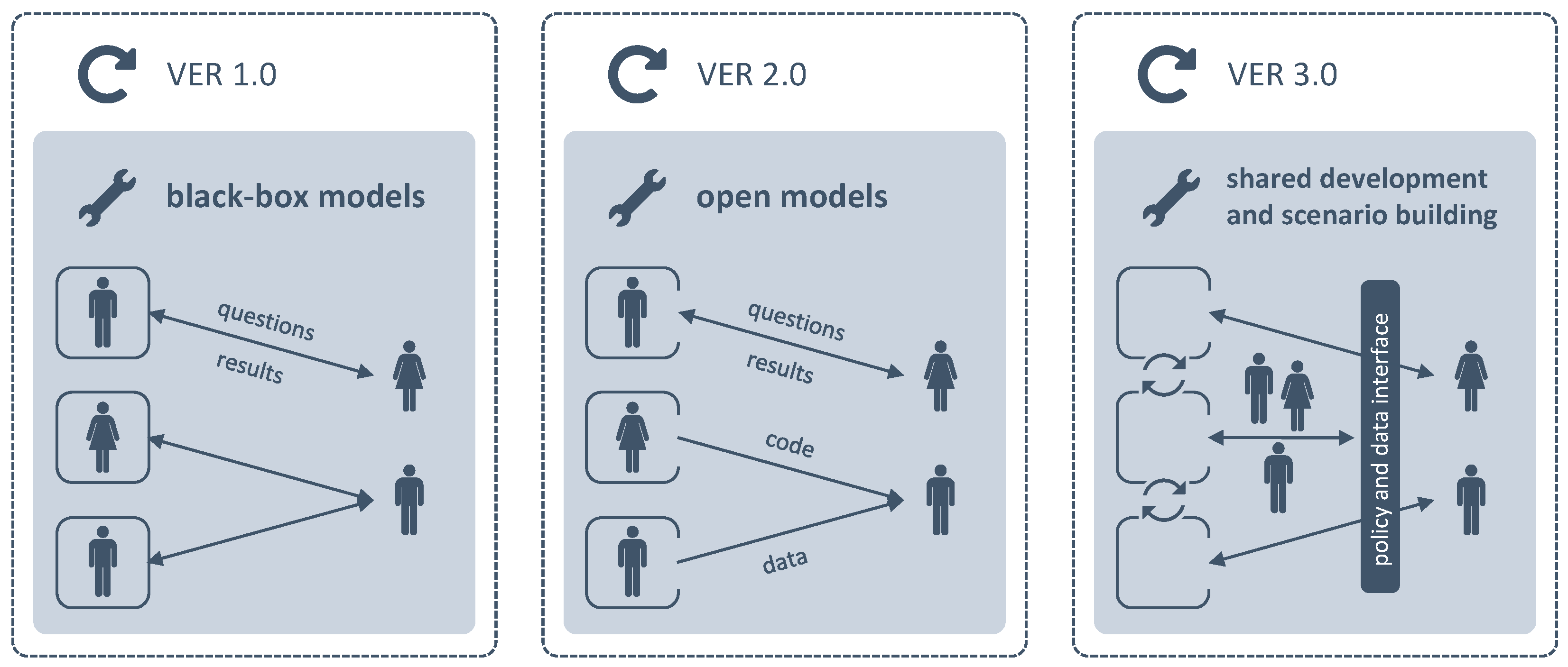
Article

Illustrating the Benefits of Openness: A Large-Scale Spatial Economic Dispatch Model Using the Julia Language

Workgroup for Infrastructure Policy (WIP), Technische Universität Berlin, H 33, Straße des 17. Juni 135, 10623 Berlin, Germany
*
Author to whom correspondence should be addressed.
Energies 2019, 12(6), 1153; https://doi.org/10.3390/en12061153
Submission received: 19 December 2018 / Revised: 17 March 2019 / Accepted: 19 March 2019 / Published: 25 March 2019
(This article belongs to the Section C: Energy Economics and Policy)

Abstract

:
In this paper we introduce a five-fold approach to open science comprised of open data, open-source software (that is, programming and modeling tools, model code, and numerical solvers), as well as open-access dissemination. The advantages of open energy models are being discussed. A fully open-source bottom-up electricity sector model with high spatial resolution using the Julia programming environment is then being developed, describing source code and a data set for Germany. This large-scale model of the electricity market includes both generation dispatch from thermal and renewable sources in the spot market as well as the physical transmission network, minimizing total system costs in a linear approach. It calculates the economic dispatch on an hourly basis for a full year, taking into account demand, infeed from renewables, storage, and exchanges with neighboring countries. Following the open approach, the model code and used data set are fully publicly accessible and we use open-source solvers like ECOS and CLP. The model is then being benchmarked regarding runtime of building and solving against a representation in GAMS as a commercial algebraic modeling language and against Gurobi, CPLEX, and Mosek as commercial solvers. With this paper we demonstrate in a proof-of-concept the power and abilities, as well as the beauty of open-source modeling systems. This openness has the potential to increase the transparency of policy advice and to empower stakeholders with fewer financial possibilities.
Dataset: 10.5281/zenodo.1044463
MSC:
90-04; 90C05; 90C90; 91B26
JEL Classification:
C61; D41; L94; O34; Q41

1. Introduction

In the wake of the strenuous efforts to reduce the effects of climate change, electricity systems worldwide have undergone profound transformations over the last decades from mostly centralized conventional power generation using carbon-intense fossil fuels towards more decentralized renewable power plants. Nevertheless, the goals of climate protection demand for further action and massive changes in the upcoming decades. In order to achieve a better comprehension of electricity systems, assess and optimize operation and investment decisions, but also to generate insights for policy making, electricity sector models are being used. These models are usually large-scale, complex techno-economic models describing the behavior of an electricity system in operation. The rapid change of the electricity sector, driven by vast extensions of renewable installations and an increase in sector coupling with heat and transportation, make them even more relevant for a consistent energy transition in the present and coming years.
Historically, most of these models have acted as proprietary black-box solutions, written in commercial systems and operated by organizations without the opportunity for other researchers to reproduce and validate results and for the public to fully understand and use these models, leading to a lack of transparency in the modeling community. One example is the European Commission’s strategic long-term vision for a climate neutral economy by the year 2050. The policy package laid out here is based on insights gained using an energy sector model that cannot be directly reproduced since neither the model source code nor the data sets have been published.
Against this backdrop, more and more voices are advocating for open source, open data, and open access in energy system modeling [1]. Some initiatives already have published their models for an open-source use (Examples are the energy modeling system OSeMOSYS [2] or the power system analysis tool PyPSA [3] and the open energy modeling framework (oemof, www.oemof.org), both written in Python. Those two models can be used fully open source, and oemof even provides a library for output visualization.).
With this paper we are presenting a new tool set for electricity and energy system modeling: the rather new programming language Julia, developed at MIT specifically for the needs of scientific computing, in combination with its algebraic modeling library JuMP. In a benchmark study with a proof-of-concept (PoC) for a fully ‘open’ electricity system model we are presenting a quantitative comparison with regard to computation time of the new Julia/JuMP with the conventional proprietary General Algebraic Modeling System (GAMS).
We argue that using an open-source language like Julia, the modeler’s efficiency and productivity can even be enhanced, since the whole modeling workflow from data pre-processing to visualization can be implemented within the same system at only very low start-up costs. Embedded into a broader open concept, this would lead to an increase in transparency but also to a strengthening of the modeling community.
On the other hand, our benchmark study also shows one deficit of open-source tools: for the time being at least, very complex models are still dependent on proprietary software in the form of the numerical solvers required since open-source alternatives can mostly not keep pace with their commercial counterparts.
With this paper we also introduce Joulia.jl, an open-source package for large-scale spacial economic dispatch problems written in Julia/JuMP, solely using open data and—where complexity allows—making use of open-source numerical solvers.
The remainder of this paper is structured as follows: Section 2 describes the benefits of open science. Section 3 provides a short introduction into the Julia programming language and the algebraic modeling language JuMP. Section 4 explains the model and gives an overview of the used input data. In Section 5 the implementation in Julia/JuMP and the results of the benchmark tests are discussed. The paper then concludes with a summary and outlook in Section 6.

2. The Benefits of Openness

In their manifesto (www.openmod-initiative.org/manifesto), the Open Energy Modeling Initiative (openmod) advocates for more openness in energy modeling:
«Energy models are widely used for policy advice and research. They serve to help answer questions on energy policy, decarbonization, and transitions towards renewable energy sources. […] We believe that more openness in energy modeling increases transparency and credibility, reduces wasteful double-work and improves overall quality. This allows the community to advance the research frontier and gain the highest benefit from energy modeling for society.»
The Open Definition 2.1 (www.opendefinition.org) states: “Knowledge is open if anyone is free to access, use, modify, and share it—subject, at most, to measures that preserve provenance and openness.” More specifically, the openness of a modeling project can affect different dimensions. We define five dimensions of openness that will be described in the following section: open data, an open-source modeling language, open-source model code, open-source solvers, and finally open-access publications. This follows recommendations by DeCarolis et al. [4] and Morrison [5]. These dimensions can be aggregated to three major topics: the availability and usage as well as publication of input and output data, the software part, and the scientific publications. See Figure 1 for a schematic overview of the workflow and the dimensions of openness in the energy modeling process.
The difference between open-source software (OSS) and closed-source software (CSS) generally lies in the availability of the source code to the general public. OSS, as promoted by the Open Software Initiative (OSI) (www.opensource.org), comes with a license with minimal or no restrictions on the (re-)distribution, use, and modification of the software. The Free Software Foundation (FSF) (www.fsf.org) and the GNU Project promote a rather similar approach:
«The word “free” in our name does not refer to price; it refers to freedom. First, the freedom to copy a program and redistribute it to your neighbors, so that they can use it as well as you. Second, the freedom to change a program, so that you can control it instead of it controlling you; for this, the source code must be made available to you.»
(GNU’s Bulletin Volume 1 No. 1, 1986)
CSS or proprietary software, on the other hand, is always distributed under a very restrictive license and as a ‘black box’ with no possibility to view the source code in order to determine the functionality.
The advantages and disadvantages of OSS vs CSS can be described using the categories customizability and control (is the software a ‘black box’ or can the user check what it does ‘under the hood’?; can the user change the source code in order to adapt the software to her specific needs?), security (can the software be corrupted by hackers?), reliability (does the software do what it promises? does it come with a huge number of bugs?), and maintenance (will bugs be fixed with a short lead time? will new features be implemented?).
Famous examples of OSS are Python as an established programming language, Julia as a rather new programming language, and OSeMOSYS [2] as an energy sector model. Infamous examples of CSS, on the other hand, are GAMS as an algebraic modeling language, and PRIMES [7] as an energy sector model.

2.1. Open Data

Energy sector models in general and electricity sector models in particular are mostly not rocket science (To quote an expert in the field: “The whole world can be modeled as linear programs!”) but are largely data-driven (hence: ‘large-scale models’). In the past, most of this data was not available to the general public, hidden in commercial databases or not accessible at all due to trade secrets and matters of ‘national security’. Over the last few years, stakeholders in the electricity sector started to open up and publish data online, in most cases because of legislation obligating them to a certain transparency. Nevertheless, while many of those data sources can now be openly viewed, it is—according to copyright law and licensing—mostly not legally possible to use, process, and redistribute this data why more and more initiatives are calling for improved legislation [8]. Nevertheless, there is and always will be a certain portion of data that will not be available to the public.
Another aspect is the structure of publication and quality of the published data. Projects like Open Power System Data (OPSD) (www.open-power-system-data.org) [9] try to tackle this issue by providing Python scripts to download and pre-process commonly needed power system data for modelers. This also increases the productivity of modelers since not everyone has to go through the same tedious process of data collection and pre-processing again [1].

2.2. Open-Source Programming & Modeling Tool

An algebraic modeling language is a modeling tool to formulate an optimization (or simulation) problem in a high-level language and then pass the generated matrix on to a so-called solver—an independent software—for calculating the numerical solution to the problem rather than writing the input directly in low-level code.
When it comes to the decision what modeling tool should be used for a project, there is a quasi standard at least for the academic and industry energy community: GAMS, the General Algebraic Modeling Language. Aside from this, AMPL can be used but there is also a whole range of viable open-source alternatives with major advantages over their commercial competitors. One of them is R, a language originally designed for statistical computing. A more general solution is Python in combination with Pyomo as an optimization library, which could be considered to be the open source standard. In this paper we propose the usage of the Julia Language in combination with the optimization package JuMP. For details on Julia and JuMP see Section 3.
The major advantage of proprietary software in the context of the used modeling language is the ease of use. Usually the software comes as an out-of-the-box solution with an IDE, ready to be used. The software is being maintained on a regular basis and everything should work reliably including the links to the solvers to be used. On the contrary, it is less customizable for example for the usage of alternative solver packages. Only supported solvers can be used with the proprietary software. Furthermore, established OSS solutions like Python with a long history and a substantial developer community come with at least the same level of reliability.
Table 1 gives an overview of the software considered in this paper and some of its characteristics.

2.3. Open-Source Model Formulation

The most important part of the process is the model formulation in the form of source code. Assessment models should not be a ‘black box’, just delivering numbers as results that are used for policy implications and that might on the way become perceived as facts by policymakers. Bazilian et al. [10] and Pfenninger et al. [1,11] all argue that energy scientist must show what happens ‘under the hood’ of their models.
This transparency is the only way other researchers, but also the general public, can replicate and validate the results and fully understand and challenge the models in the peer-review of publications but also in the context of policy advice. This is also the only way to fulfill the standards of open science. Furthermore, it increases the quality of models since developers are forced to decrease the number of errors or at least errors can be found by others. The models therefore become more robust.
Especially when it comes to the usage of model results as arguments for certain policy implications or recommendations, the credibility and legitimacy of those results increases significantly if everyone is able to check them and to see the underlying assumptions.
Last but not least, publishing models according to open standards grants access to anyone and therefore also to stakeholders with less financial means like non-governmental organizations or developing countries, enabling them to produce their own analyses. It also fosters the interoperability of different models [12].
Pfenninger et al. [13] supply a guideline of strategies on how to open models up, while Hülk et al. [14] provide a transparency checklist for models. Several meta studies describe the current questions and challenges of electricity and energy sector modeling [12,15,16].

2.4. Open-Source Numerical Solver

For numerically solving large-scale problems—like electricity sector models—commercial solvers are usually the product of choice for most modelers. Commonly known solver packages are the CPLEX Optimizer by IBM and Gurobi by Gurobi Optimization but also less well-known products like MOSEK by Mosek ApS can be used. For academics at universities these products are usually free of charge under academic licenses, while research institutes, government agencies, non-governmental organizations, and commercial users must purchase commercial licenses.
Open-source solvers can—under certain circumstances—be an alternative. In this paper we are benchmarking a number of open projects against the commercial ones. The advantages in those cases are similar to the ones for the modeling tool: publicly available and therefore controllable (no ‘black box’) source-code as well as cost savings for license fees. Standard open-source solvers for linear programs are CLP by COIN-OR and GLPK by the GNU Project. Another promising product is ECOS by embotech, a spin-off of ETH Zurich.
Since CLPEX and Gurobi are, by now, well established products with high license fees and therefore bigger resources than open projects, their performance in solving problems is usually many times better. Nevertheless we wanted to use open-source solvers as a proof-of-concept: it is possible and—depending on the size of the project—worthwhile to cover the complete modeling workflow with open solutions. This point is especially important for users or stakeholders with very little budget like non-governmental organizations or even developing countries.

2.5. Open-Access Publications

Last but not least the outcome of a model should be freely available to stakeholders and the interested public as open-access publications (like this one is). Due to the coersions of the established valuation system, many academics are still publishing their works in commercial journals, available to others only by means of paying high subscription or usage fees. Most of the published research has been funded by taxpayer’s money and results should therefore be available to all citizens and the general public free of charge. The publication of open-access articles—most favorably in fully open-access journals—should be the academic standard. According to the European Competitiveness Council (COMPET), all publicly funded scientific papers should be published open-source by 2020. Already today, collaborators in EU Horizon 2020 research projects have the obligation to publish open access. In October of 2018 OpenAIRE, funded by the European Commission since 2008, has been established as a non-profit organization democratizing the research life-cycle, by "assisting the transition of how research is performed and knowledge is shared” (www.openaire.eu). They for example support and offer services and infrastructure like the Zenodo repository service (www.zenodo.org) for publishing research data.
In this section we have introduced five key dimensions that are a prerequisite of fully open energy science. These include open data, open-source programming and modeling languages, open-source model code, open-source solvers, and open-access publications. While open-source tools—aside from numerical solvers—are already today capable of the tasks, a lot of challenges still remain [6]. One of them is practical knowledge of the stakeholders. Others include the need for collaboration, poor data quality, and the issue of licensing to be able to re-use data and code. The costs related to proprietary software like GAMS do not seem to be a driver in the game.

3. The Julia Language & JuMP.jl

The model described in this paper is written in the Julia programming language [17] and uses the package JuMP.jl [18] as an algebraic modeling library, in combination with several packages serving as links to the examined solvers. The integration of the algebraic modeling language directly into high-level programming languages comes with the major advantage that other functionalities of the language like data pre- and post-processing as well as visualization can be used, representing the full modeling workflow (compare Figure 1) within the same code. This methodology is comparable to the more established combination of Python as a programming language with Pyomo as its algebraic modeling library.
Julia is a high-level, high-performance dynamic programming language for numerical computing. It is the ideal combination of practical, yet rather slow high-level dynamic languages like Python, R, or Mathematica and efficient but statically typed languages like C and Fortran. With its sophisticated type system, just in time compilation, and other measures it combines the productivity and efficiency of both worlds. Libraries for Julia can be written entirely in the Julia language itself. Julia is fully open source and has a rapidly growing community of users and developers (more than 500 contributors and more than 1200 packages available) [17] with a very open-minded, diverse, and welcoming community. In August 2018, after six years of development, the official version 1.0 has been released, leading to a steep growth in number of users and popularity. By the end of 2018, the GitHub repository containing the core language had more than 19,000 ‘stars’, that is, GitHub users who follow the repository. It is listed among the top 50 programming languages according to the Tiobe index. Yet, given the short history of the language, it has not reached the same level of maturity as Python. The same holds true for JuMP.jl, which is currently available in version 0.18 with a major transition coming up with version 0.19 in March of 2019.
Julia can be used in a REPL (read-eval-print loop) on a console, in Jupyter notebooks, and in IDEs like the Atom text editor. Since data pre- and post-processing, modeling, and visualizations can be written all within Julia, the complete workflow of a modeler can be represented within the system boundaries (as in Python). The package JuMP.jl (Julia for Mathematical Programming) provides the user with a very efficient and fast algebraic modeling language. It builds upon the existing syntax of Julia and uses code-generating macros to describe variables, objectives, and constraints. The necessary code is therefore compact and legible.
Since Julia needs some time for the first compilation, there is a start-up cost to be accounted for. Running the same or similar models in loops brings down the time of model generation significantly. Benchmarking JuMP against other open-source and commercial languages shows that is is significantly faster than the open-source solutions like Pyomo and, depending on the problem, in the same range or better than commercial solutions like GAMS [18,19]. Hence, one of the main advantages of Julia is speed, which this paper is testing for an application in electricity sector modeling.

4. Model Description

The model used in this paper replicates an electricity market by solving an economic dispatch problem—that is, minimizing total system generation costs—including power flows on a high-voltage transmission network. Therefore, supply and demand are held in balance on a nodal basis. Supply is represented by a hourly merit order of thermal and renewable power plants as well as the possibility or energy storage. Exports and imports from neighboring countries (or market zones) are also taken into account. As results the model outputs the production levels of generation units, the filling level of storages, nodal market clearing prices, as well as power flows on transmission lines—all on an hourly basis. Figure 2 gives an overview of the model structure. Section 4.1 outlines the used data, Section 4.2, Section 4.3, Section 4.4, Section 4.5 and Section 4.6 describe the equations the model is comprised of. Please refer to Appendix A for a declaration of the used symbols.
In this paper we are comparing the implementation of this model as linear programs (LPs) in two different modeling tools or languages. For the implementation in GAMS we use ELMOD-DE, developed by Egerer [20] for the German electricity market. The source code is published open source (www.diw.de/elmod) (together with a reference data set for the year 2012), which is why we decided to use this implementation in our benchmarking test for the sake of replicability. ELMOD-DE is based on the original version of ELMOD, an European electricity market model developed by Leuthold et al. [21]. For the implementation in Julia we use Joulia.jl, introduced in Section 5.1.

4.1. Input Data

The model in both implementations uses the same reference data set for the German electricity market for the year 2015 [22] (without gas and heat). Details of the data set are described in the accompanying data documentation [23] (Chapter 2). The data set is composed of the following parameters:
  • 724 high voltage transmission lines with their geographical information, voltage levels, and transmission limits (see Figure A1)
  • 450 network nodes with their geographical information and installed renewable capacity
  • 707 conventional power plant blocks with their geographical information, technology, fuel, installed capacity, efficiency, emissions, and (if applicable) transportation costs for hard coal
  • electricity demand time series for each node
  • import and export time series for electrical neighbors
  • availability factors for conventional generation capacity by technology
  • availability time series for renewable generation capacity by technology
Some relevant details of the data set are listed in Appendix B. Figure A1 shows a map of the transmission lines considered in the model. Table A4 gives an overview of the aggregated installed capacity in the German market for the model. Table A5 shows the annual average of fuel costs for conventional generation capacities as well as their carbon intensity and annual average price of emission allowances.
It is obvious that the complexity of the model (and therefore the runtime) is mostly driven by the size of the electricity system analyzed. Section 5.2 illustrates the correlation.

4.2. Objective

The objective of the model is to deterministically minimize total system costs in terms of generation costs by a benevolent planner with perfect foresight. Hence, the objective function is to minimize the sum of all hourly conventional generation G p , t , multiplied by the associated specific variable costs v c p , t of the specific power plant block (Equation (1)). Renewables are assumed to have zero marginal costs.
min cost G , R , p h e s G , p h e s D = p , t G p , t × v c p , t

4.3. Energy Balance

Equation (2) describes the nodal energy balance. Generation from conventionals G p , t , renewables R n , s , t , and pumped hydro storages p h e s G p h e s , t connected to the node as well as the netinput n n θ n n , t × b n , n n from the transmission grid and possible exchanges with neighboring market zones e x n , t have to be in balance with electricity demand d n , t and demand from pumped hydro storages p h e s D p h e s , t at all network nodes and at all times (hourly resolution) in order to satisfy all demands and keep the system stable. Nodal market clearing prices are derived from the dual variables of the energy balance.
p G p , t + s R n , s , t + p h e s p h e s G p h e s , t + n n θ n n , t × b n , n n + e x n , t = d n , t + p h e s p h e s D p h e s , t n , t

4.4. Generation

The generation G p , t from each block p of a conventional power plant is limited by the maximum installed capacity g ¯ p which is reduced by an availability factor a v a g p , t (Equation (3a)). Equation (3b) for generation from intermittent renewable sources R n , s , t works analogously, only that the installed capacity r ¯ n , s is aggregated by network node n and technology s and multiplied by a weather-dependent availability time series a v a r n , s , t .
G p , t g ¯ p × a v a g p , t p , t
R n , s , t r ¯ n , s × a v a r n , s , t n , s , t

4.5. Storage

The model considers pumped hydroelectric energy storage (PHES) in Equation (4). The inter-temporal constraint in Equation (4a) links the filling level p h e s L e v e l at time t to the level at time t 1 , considering generation p h e s G p h e s , t and pumping p h e s D p h e s , t from the PHES. Due to losses in the storage cycle, the PHES demand is multiplied by an efficiency factor e f f p h e s . Equations (4b) and (4c) limit the generation and pumping from a PHES unit to the maximum installed capacity g s t o ¯ p h e s , while Equation (4d) limits the storage filling level to the maximum energy content l s t o ¯ p h e s of a PHES. For reasons of parallelization, the model assumes each PHES to be empty at the beginning and end of each model week in order to avoid a hard link between weeks.
p h e s L e v e l p h e s , t = p h e s L e v e l p h e s , t 1 + e f f p h e s × p h e s D p h e s , t p h e s G p h e s , t p h e s , t
p h e s G p h e s , t g s t o ¯ p h e s p h e s , t
p h e s D p h e s , t g s t o ¯ p h e s p h e s , t
p h e s L e v e l p h e s , t l s t o ¯ p h e s p h e s , t

4.6. Transmission Network

The transmission network is represented using the DC load flow approach [24] (p. 313) (Equation (5)). Only considering the real power flow and assuming small differences in voltage angles θ and voltage levels, this linearization of AC power flows provides an—for this application—acceptable level of accuracy (This methods is accurate on average but there can be significant flow errors on certain lines, see [25] (Chapter 6) for details.)
The modulus of the power flow P F l , t on a line l is limited by the maximum power flow p f ¯ l for this line (Equation (5a)). This maximum power flow accounts for N-1 security, applying a transmission reliability margin, and is determined by its voltage level and number of circuits. This power flow P F l , t is calculated summing up the multiplications of the voltage angle θ n , t of a node with the corresponding entry of the adjacency (node-to-line) matrix h l , n for this line (Equation (5b)). The n e t i n p u t n , t used in the nodal energy balance is calculated with the same scheme, only this time summing up the multiplications of the voltage angle θ n n , t with the network susceptance matrix b n , n n for all other nodes n n in the network (Equation (5c)). Finally, Equation (5d) defines a slack bus n ^ with a voltage angle of zero to be the reference point of the network.
| P F l , t | p f ¯ l l , t
P F l , t = n θ n , t × h l , n l , t
n e t i n p u t n , t = n n θ n n , t × b n , n n n , t
θ n ^ , t = 0 t

5. Implementation & Results

5.1. Joulia.jl

An overview of existing proprietary electricity sector models can be found in Foley et al. [26] and Carramolino et al. [27]. With GenX, the MIT Energy Initiative contributed an extensive model written in Julia [28], but the source code is not publicly available. With 
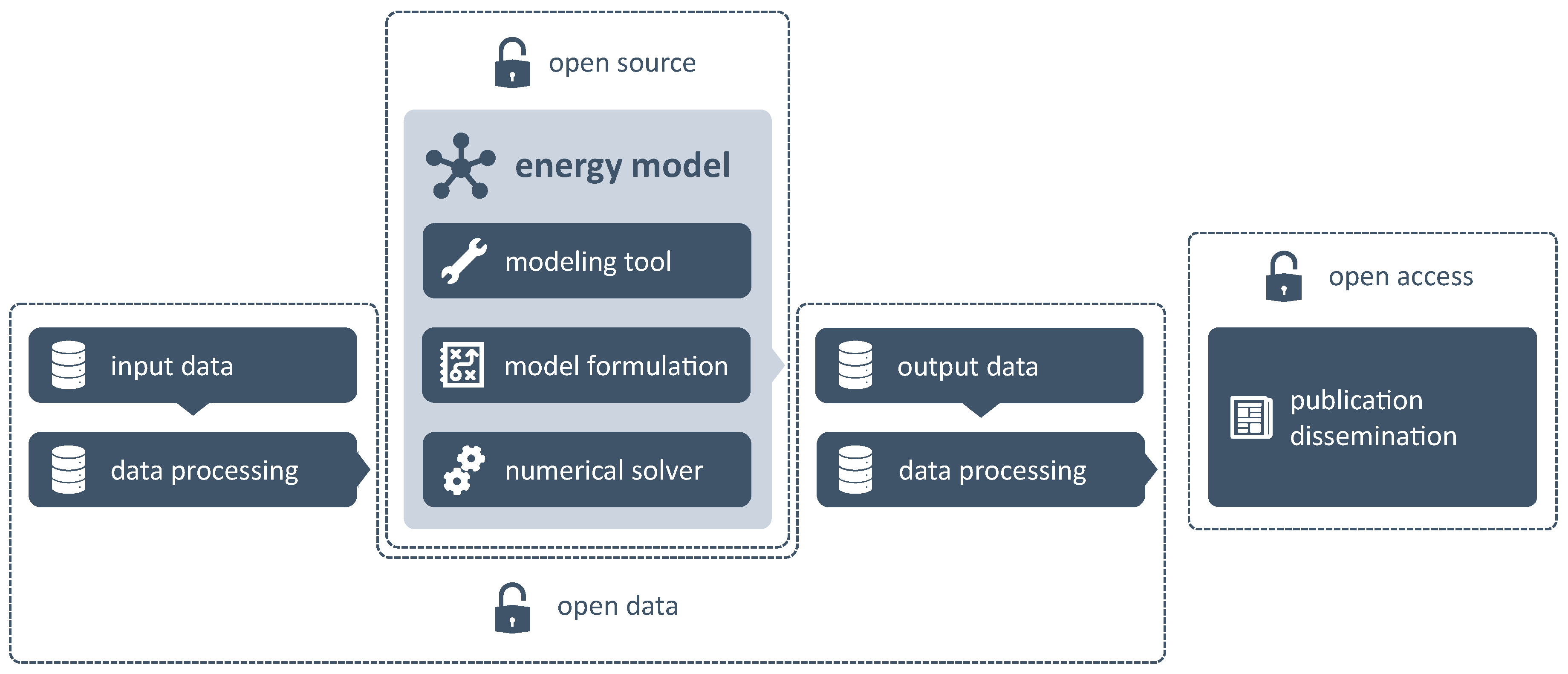
Joulia.jl we want to contribute to the community an energy sector model fulfilling the criteria of all five dimensions of openness according to Section 2. It should be easily usable for everyone, the first one written in the cutting-edge Julia language, providing all the tools for the entire modeling pipeline and coming with open data ready to be used.
Joulia.jl is a package provided within the JuliaEnergy organization on GitHub (www.github.com/JuliaEnergy/Joulia.jl), easily to be imported to the Julia environment. It uses the library JuMP as an algebraic modeling tool or language. The package provides the user with generic functions that together constitute the electricity market model described in Section 4.
Depending on further packages, any desired data set can be read in from .csv files or binary files. Joulia.jl hereby uses a generic, technology-neutral and extendable data framework in order to be able to extend the future functionality. The model functions can then be called with the data set, generating the actual full model code thereof and passing it on to a desired solver. Results from the solver are being collected and used to produce visualizations, profiting from the plot packages of Julia. Even dynamic plots are possible.
Joulia.jl can be used for a number of research questions, for example the impact of nodal prices and of different configuration of price zones (see [29] for a possible application). It can be used to analyze the impact of investment decisions into generation or transmission capacities on generation levels by technology, line flow patterns, as well as price levels. Using different data sets, the geographic scope of the model can be extended for example to the whole of Europe or to any other region like developing countries in order to assess policy changes in their markets.
Listing 1 shows a code example representing Equation (2) (In order to capture possible lost generation or load, a dummy variable is introduced into the equation.). JuMP’s @constraint macro adds an equality constraint called market_clearing to the model named m for each n N and t T . Listing 2 juxtaposes the same equation in its GAMS implementation. Here, the equation has to be declared and defined first, using the EQUATION keyword before it can be initialized in a second step following the .. operator. Using the sum operator, the set over which the summation should be executed can be limited by the $ operator. The same effect can be generated in Julia using in-line for loops. Another difference is the assignment of equations to models. In GAMS the model can be defined at the very end of the code and initialized with a list of equations. In JuMP, a variable or an equation is directly linked to a model initialized in the beginning. Nevertheless different models are possible, consisting of the same variables and equations only written out once if the model is generated using functions. It can be stated that in general models in JuMP are more compact then their counterparts in GAMS, as illustrated by an example in [18].
Listing 1. Example code for market clearing/energy balance constraint in Julia/JuMP.
Energies 12 01153 i001
Listing 2. Example code for market clearing/energy balance constraint in GAMS.
Energies 12 01153 i002
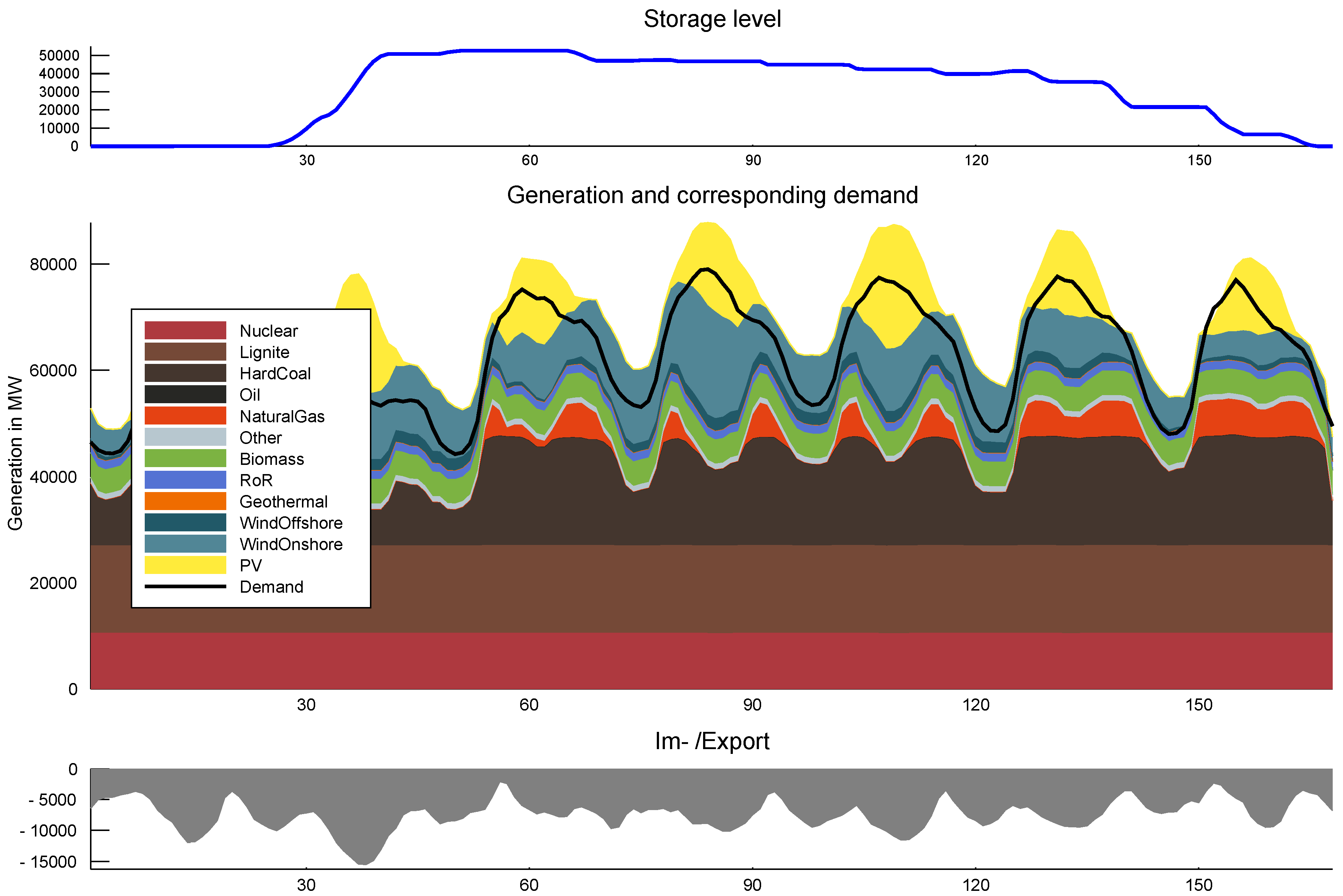
Figure 3 shows an example of the resulting cumulative dispatch for each hour in one week in summer, broken down by fuel and renewable source, respectively. The black line shows electricity demand while imports and exports are represented by the gray area in the bottom subplot and the filling level of pumped hydroelectric storages is mapped in the top subplot in dark blue.
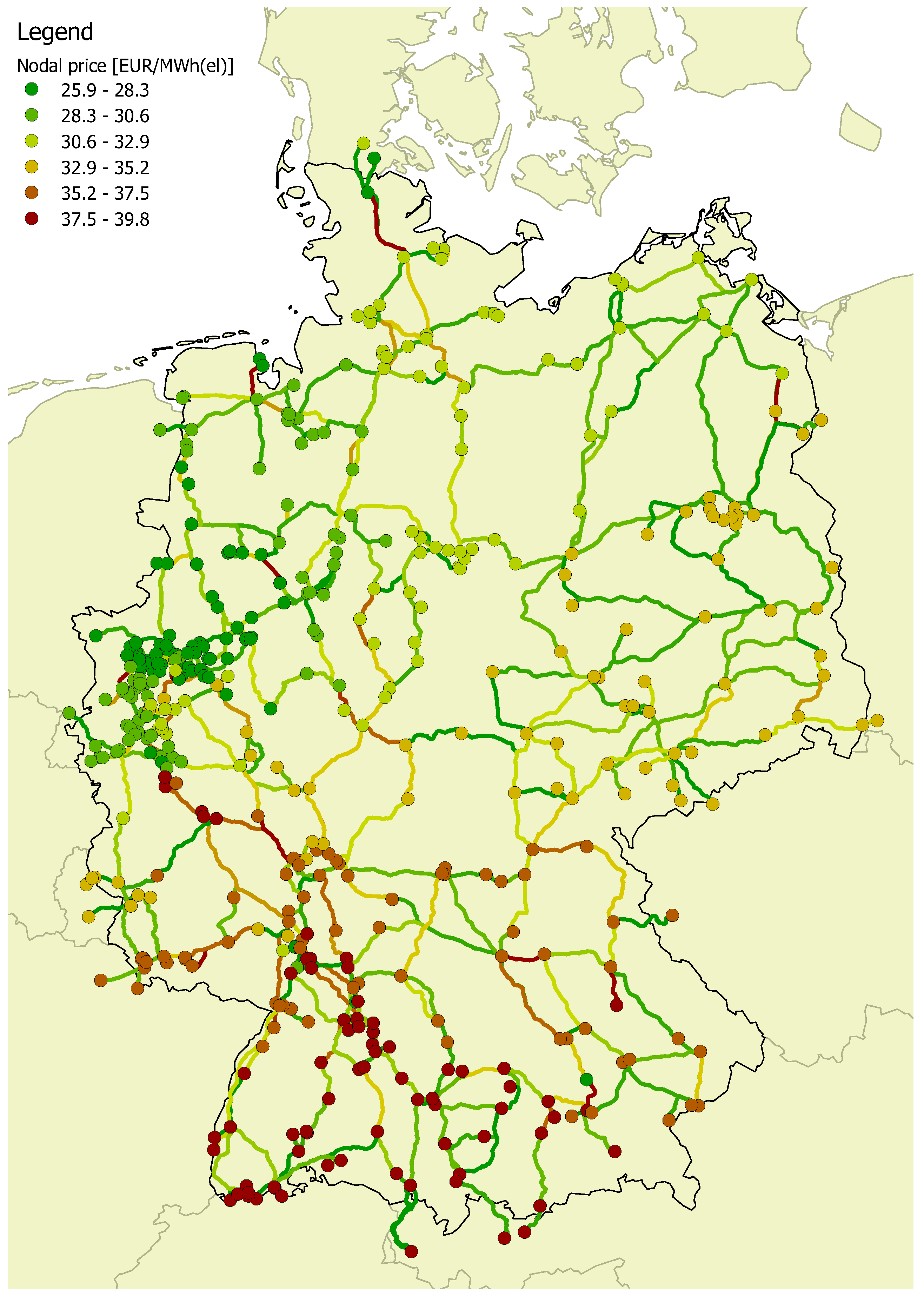
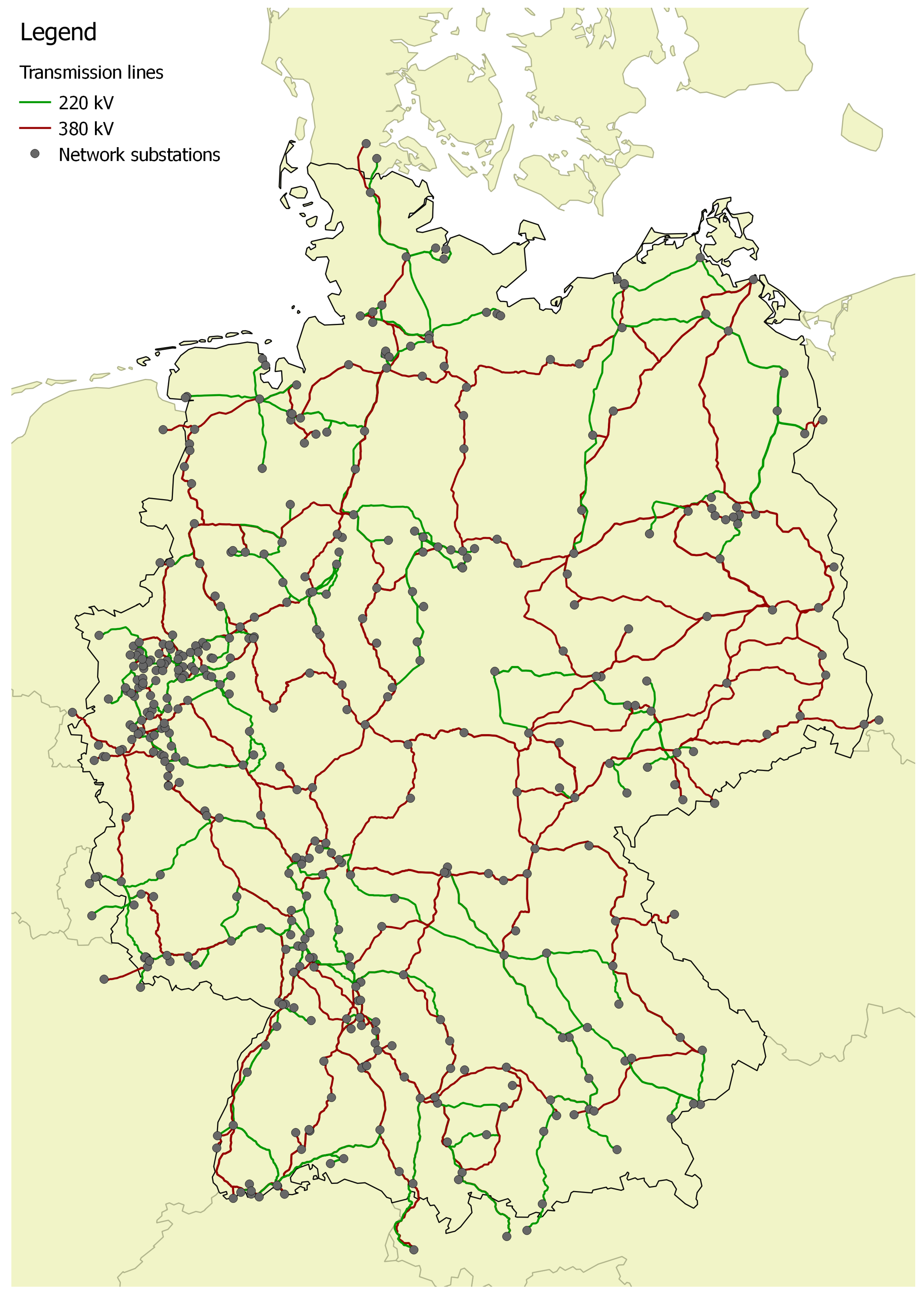
Since the transmission system is also available with its geographical information, the utilization of the lines and the calculated nodal prices in the model can be visualized as in Figure 4.

5.2. Benchmark Test

In a benchmark test we are comparing the implementation of the model in GAMS (ELMOD-DE), solved with the three commercial solvers CPLEX, Gurobi, and Mosek with the implementation in Julia/JuMP (Joulia.jl), solved with the same three solvers plus the additional two open-source solvers ECOS and CLP not available in GAMS. In order to visualize the impact of the complexity of the problem on the runtimes we distinguished three cases: (i) a simple case for dispatch without storage (and hence no intertemporal constraints) and no transmission grid (only Equations (1)–(3)), (ii) a medium case, adding storage (Equation (4)), and (iii) a hard case, adding the transmission grid (Equation (5)).
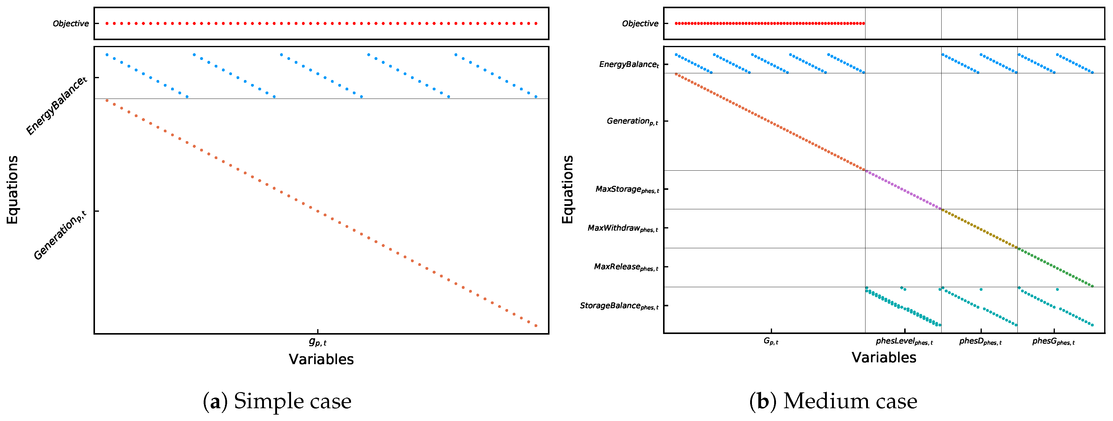
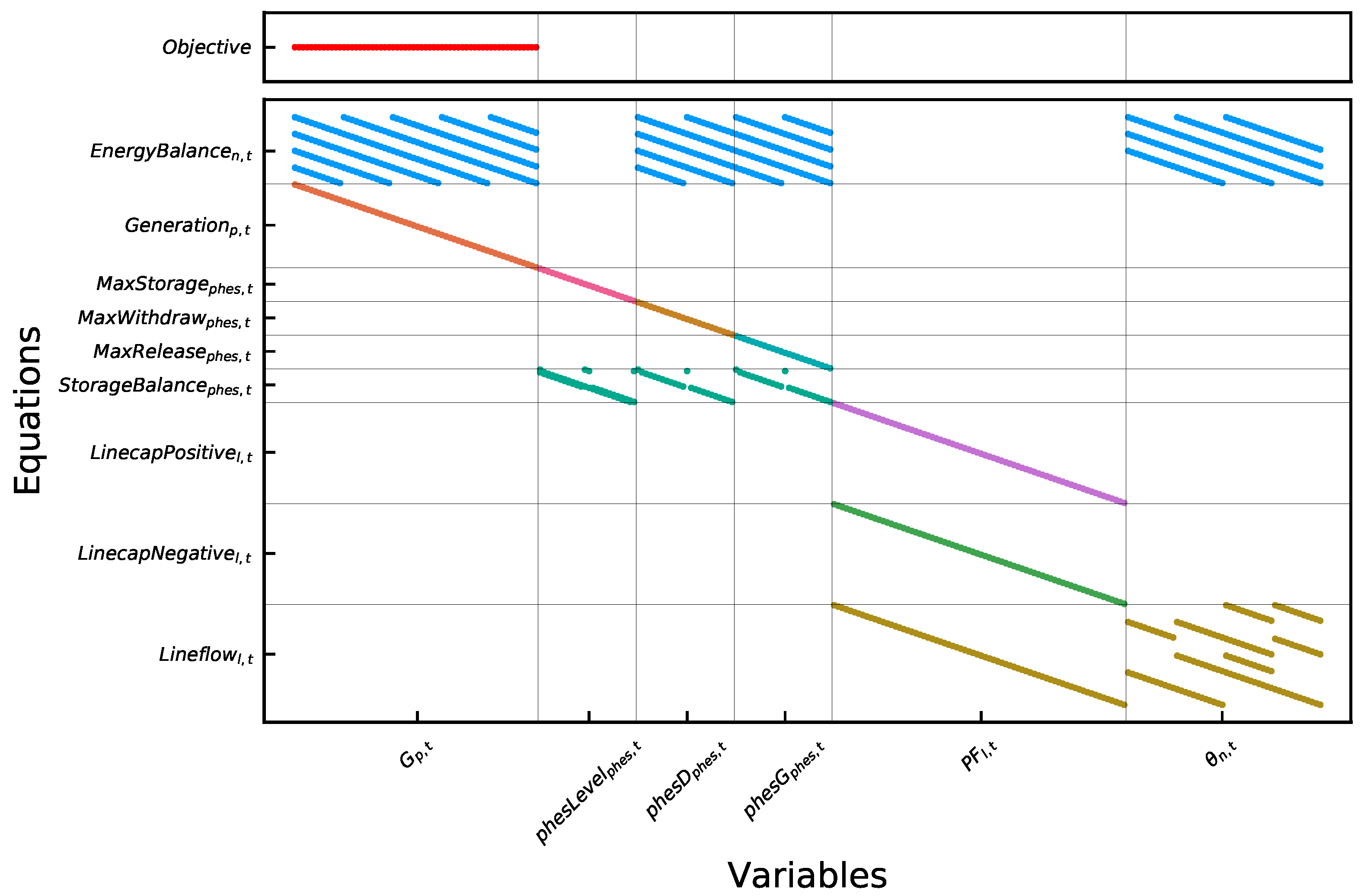
In order to illustrate the difference of these three cases, the constraint coefficient matrix of the problems can be analyzed. Since the original problem is too expansive to be plotted, we generated a sample problem consisting of only five power plant blocks, four network nodes, six network lines, and three storage units. This problem only calculates the dispatch for twelve time slices. Figure 5a shows the resulting matrix of the simple case. Each dot in the graph represents the occurrence of the variable G p , t in one of the equations, that is, a non-zero element of the matrix. Each increase in t or p expands the matrix accordingly. In Figure 5b the resulting matrix for the medium case is shown. The top left corner contains the matrix of the simple problem. The additional variables and constraints for the storages expand the matrix to the right and downwards, quadrupling the size of the matrix. Again, each increase in t or p h e s expands the matrix additionally. Adding the power flow constraints of the transmission network, the matrix results in Figure 6. The matrix of the medium case is included in the top left corner again, representing only one quarter of the full matrix. Now, an increase in n or l would expand the matrix additionally. This simple example shows how the hard problem is already 16 times larger than the simple problem.
Now, taking into account the actual sizes of the used sets according to Section 4.1, the numbers are put into perspective: The Joulia.jl simple problem consists of 308,112 rows, 308,280 columns, and 616,224 non-zeros, the medium problem of 329,616 rows, 324,408 columns, and 664,608 non-zeros, and the hard problem of 770,112 rows, 673,008 columns, and 1,729,056 non-zeros. The GAMS problem structure is almost—but not perfectly—identical due to minor differences in building the LP files. This has no significant influence on the benchmarking test, though.
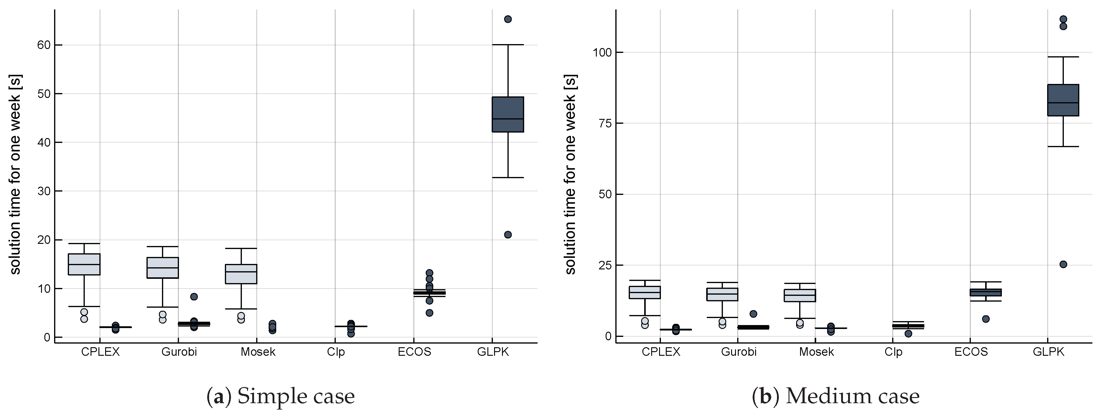
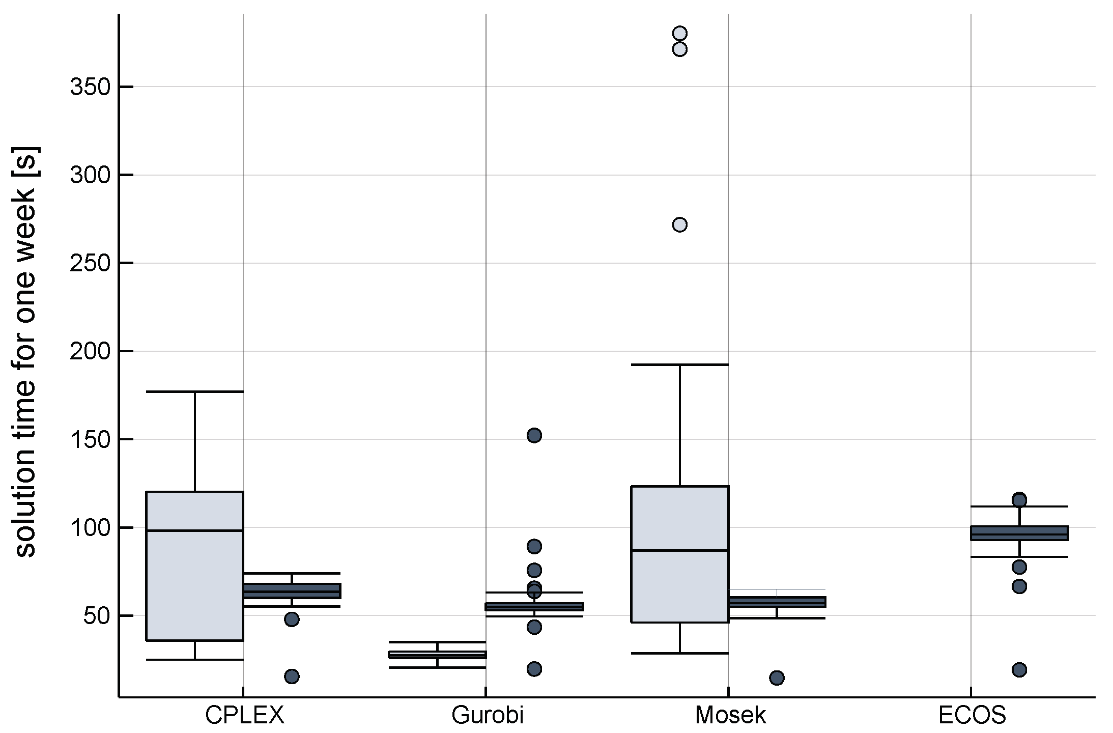
Figure 7 and Figure 8 show box plots of the total run time of solutions for all the weeks of one year with the named combinations and the three cases. Table 2 summarizes the solve statistics for the hard case. For reasons of comparability, the total time for building the model and solving it is being used since GAMS and Julia are using different metrics in that regard. The calculations were made with Julia version 1.0.2, JuMP version 0.18.5, GAMS version 25.1.3, CPLEX version 12.8, Gurobi version 8.1, and Mosek version 8.1.
Obviously, the size and complexity of the model to be solved totally depends on the extent of the data used. Therefore, benchmarking tests on optimization problems can only give an indication on the proportions and magnitudes but cannot easily be generalized. Yet, the literature for similar benchmarking tests involving commercial and open-source solvers shows that commercial solvers are always the faster alternative, while open-source solvers cannot match their performance but—depending on the problems tested—capable ones are available if the commercial alternatives are not a viable option.
Meindl and Templ [30] give an overview of existing open-source as well as commercial solvers for linear problems. They conduct a case study solving 200 instances of the secondary cell suppression problem. These instances can be divided into an easier and a harder group. Generally, they find that both tested commercial solvers CPLEX and Gurobi perform better than the open-source solvers CLP, GLPK, and LP_solve. However, when solving the group of easier instances, GLPK and CLP were only nine and 13 times slower than the fastest solver (CPLEX). The gap widened between the solvers as CLP took 2823 times the run time of CPLEX in the harder cases. Also, Gurobi performed much worse, only being a bit faster than GLPK.
Jablonsky [31] benchmarks the three commercial solver CPLEX, Gurobi, and FICO XPRESS on a set of 361 mixed integer problems. The results vary between the different instances of problems but overall Gurobi performed best in most cases.
Gearhart et al. [32] test the four open-source linear programming solver CLP, GLPK, LP_solve, and MINOS against the commercial solver CPLEX. Firstly, they use a set of 180 linear problems which is considered as “easy”. In this run CLP was almost as fast as CPLEX. GLPK also showed a good performance with only being about nine times slower compared to CPLEX. The other two had considerably worse solution times. In the second test they benchmark only the CLP solver against CPLEX with a set of 21 “hard” problems. With CPLEX generally being better, CLP was faster in some of these instances.
In an ongoing benchmarking project by Mittelmann [33,34], several open-source and commercial solvers are tested using the Simplex and the Barrier algorithm for linear problems. Results indicate that Gurobi is the fastest and most reliable solver in both cases closely followed by XPRESS. Also, CLP is almost as fast as CPLEX in the Simplex algorithm comparison.
CLP is especially named in the literature as a very fast open-source solution, with GLPK coming in second. While we found that CLP can solve our problem, it did so in a more than 50-fold increase in average time compared to Gurobi as the fastest commercial solver and a more than 40-fold increase compared to CPLEX for the hard case. GLPK was not able to produce a solution in an acceptable amount of time for this case and showed significant shortfalls also for the simple and medium cases. The open-source solver that was able to keep pace with its competitors is ECOS with only a less than twofold increase in average time compared to the fast commercial solutions. This solver is not covered by any of the common benchmark tests.
Comparing across platforms, Julia produces on average faster results than GAMS using CPLEX and Mosek, but is a little slower for Gurobi. What is interesting is the difference for the minimum runtime for one week and the minimum runtime for full weeks only, since weeks 1 and 53 are trunk weeks with less hours. Julia is significantly faster here than GAMS. This is illustrated by the lower outliers in the box plot for Julia. Another interesting observation is the higher variability between weeks for solution times for Mosek and CPLEX with GAMS compared to Julia. Since GAMS is proprietary software, the differences cannot easily be explained (Since this paper focuses on an application in the electricity sector modeling, it is out of the scope of the paper to explain the differences in efficiency based on the low-level differences between GAMS and JuMP.). Julia/JuMP seems to have a more efficient model generation and, in part, faster links to the solvers. Since the underlying MathProgBase.jl as low-level interface will be replaced by the novel MathOptInterface.jl starting from version 0.19 of JuMP, further increases in performance can be expected.
We also tested other non-commercial solvers that are compatible with JuMP—Bonmin, Couenne, Ipopt, and SCS—but none of those were able to either solve the problem at all or to solve it in a runtime close to the solvers shown in Table 2.

5.3. Discussion

In order to deliver a comparable scope of functionality like other open-source power sector models, for example PyPSA [3] or oemof written in Python, further research in the field is necessary. In the next steps, DC transmission lines will be included and Joulia.jl will be developed from a LP model towards the integration of unit commitment decisions in a mixed integer program (MIP) variant for a better technical representation of power plants. Also, the use of heat generated from turbines will be included with a detailed representation of combined heat and power (CHP) plants. The model will also be extended by a congestion management module. Future research into the stochastic representation of the German rolling-planning market scheme of day-ahead, intra-day market, and congestion management as well as the possibility for endogenous investment decisions is intended.
Joulia.jl is intended for the open-source community with the possibility for interoperability with existing models but also for a future further development by the community, following the proposition of DTU and RLI for the third generation of energy system modeling with shared model development and scenario building (see Figure 9).

6. Conclusions

In this paper we introduce the Julia package Joulia.jl, providing a modeling framework for electricity system models, implementing the modeling workflow from processing input data, building and solving the model, and finally producing visualizations of the results. It is open source and free to use for everyone as a package on GitHub, written in and for the cutting-edge Julia language and hence providing all the tools for the entire modeling pipeline. It also comes with a free and open data set that can be used for analysis.
In order to benchmark the new modeling tool Julia as an open-source programming language in combination with its algebraic modeling library JuMP, we compare the performance of the tool in terms of runtime against an implementation of the same model in GAMS as a proprietary tool. One of the aspects examined is the possibility to use open-source numerical solvers that comes with JuMP. We have shown that the use of such open-source alternatives like ECOS is possible for the given model, with runtimes within the same order of magnitude as commercial solvers—even though the linear program can be solved a little faster using the commercial Gurobi or CPLEX. With growing complexity of models, commercial solvers are increasingly playing out their advantages of speed, with open-source solvers falling behind. Yet, comparing across platforms, open-source tools like Julia/JuMP or Python/Pyomo provide a more than viable alternative to the commercial tool GAMS, coming with other additional advantages like modern syntax and tools for data processing as well as visualization. A slight drawback is the persistent dependency on commercial numerical solvers.

Author Contributions

J.W. and M.K. both curated the data and developed the model and methodology. J.W. initiated the research, wrote the paper, and managed the review and editing process.

Funding

This work was carried out as part of the project “Long-term planning and short-term optimization of the German electricity system within the European framework: further development of methods and models to analyze the electricity system including the heat and gas sector”, funded through grant “LKD-EU”, FKZ 03ET4028A, German Federal Ministry for Economic Affairs and Energy.

Acknowledgments

The authors would like to thank Jonas Mugge-Durum for his support in bibliographic research, Bobby Xiong for his graphic support, and João Gorenstein Dedecca as well as participants and reviewers of the OR Conference 2017 in Berlin, YEEES 2018 in Delft, and JuliaCon 2018 in London for valuable comments and reviews of earlier versions. The usual disclaimer applies.

Conflicts of Interest

The authors declare no conflict of interest other than their praise for the Julia language.

Abbreviations

The following abbreviations are used in this manuscript:
CSSClosed-Source Software
GAMSGeneral Algebraic Modeling System
IDEIntegrated Development Environment
JuMPJulia for Mathematical Programming
LPLinear Program
OSSOpen-Source Software
PHESPumped Hydroelectric Energy Storage
QPQuadratic Program
SKECoal Equivalent

Appendix A. Description of Used Symbols

Appendix A.1. Sets

Table A1. Model sets.
SetDescription
ltransmission network lines
n/nntransmission network nodes
ppower plant blocks
p h e s pumped hydroelectric storages
srenewable generation technologies
ttime steps

Appendix A.2. Parameters

Table A2. Model parameters.
ParameterDescription
g s t o ¯ p h e s maximum generation/pumping capacity of PHES
g ¯ p installed conventional capacity
l s t o ¯ p h e s maximum PHES energy content
p f ¯ l power flow limit
r ¯ n , s installed renewable capacity
θ n , t voltage angle
a v a g p , t availability of conventional capacity
a v a r n , s , t availability of renewable capacity
b n , n n network susceptance matrix
d n , t electricity demand
e f f p h e s efficiency of a PHES
e x n , t exchange with electrical neighbors
h l , n flow sensitivity matrix
v c p , t variable generation cost

Appendix A.3. Variables

Table A3. Model variables.
VariableDescription
G p , t generation from conventional power plant block
P F l , t power flow on a transmission line
p h e s D p h e s , t demand from a PHES
p h e s G p h e s , t generation from a PHES
p h e s L e v e l p h e s , t storage filling level of a PHES
R n , s , t generation from renewable energy source
θ n , t voltage angle

Appendix B. Input Data

Appendix B.1. Generation

Table A4. Installed conventional and renewable generation capacity by fuel/technology [23].
FuelInstalled Capacity [MWel]Renewable TechnologyInstalled Capacity [MWel]
Nuclear12,075Run-of-river hydro3700
Lignite20,901Wind onshore41,242
Hard coal28,571Wind offshore3263
Natural gas23,625Solar PV39,332
Oil3675Biomass6900
Waste1631Geothermal33
Other fuels2466
Pumped storage8789
Total101,732Total94,312
Table A5. Annual fuel cost data for 2015 and carbon intensity [23].
Fuel CostsCarbon Factor
[EUR/t SKE][EUR/MWhth][t CO2/MWhth][EUR/MWhth]
Uranium-3.00-
Lignite-3.100.3993.03
Hard coal68.008.350.3372.56
Natural gas185.0022.730.2011.53
Fuel oil (light)373.0045.820.2662.02
Fuel oil (heavy)180.0022.110.2932.22
Emission allowances7.59 EUR/t CO2

Appendix B.2. Transmission Network

Figure A1. The German high voltage transmission network (nodes & lines). Source: [23].
Energies 12 01153 g0a1

References

  1. Pfenninger, S.; DeCarolis, J.; Hirth, L.; Quoilin, S.; Staffell, I. The importance of open data and software: Is energy research lagging behind? Energy Policy 2017, 101, 211–215. [Google Scholar] [CrossRef]
  2. Howells, M.; Rogner, H.; Strachan, N.; Heaps, C.; Huntington, H.; Kypreos, S.; Hughes, A.; Silveira, S.; DeCarolis, J.; Bazillian, M.; et al. OSeMOSYS: The Open Source Energy Modeling System: An introduction to its ethos, structure and development. Energy Policy 2011, 39, 5850–5870. [Google Scholar] [CrossRef]
  3. Brown, T.; Hörsch, J.; Schlachtberger, D. PyPSA: Python for Power System Analysis. J. Open Res. Softw. 2018, 6, 4. [Google Scholar] [CrossRef]
  4. DeCarolis, J.F.; Hunter, K.; Sreepathi, S. The case for repeatable analysis with energy economy optimization models. Energy Econ. 2012, 34, 1845–1853. [Google Scholar] [CrossRef]
  5. Morrison, R. Energy system modeling: Public transparency, scientific reproducibility, and open development. Energy Strategy Rev. 2018, 20, 49–63. [Google Scholar] [CrossRef]
  6. Müller, B.; Weibezahn, J.; Wiese, F. Energy modelling—A quest for a more open and transparent approach. Eur. Energy J. 2018, 8, 18–24. [Google Scholar]
  7. E3MLab. PRIMES Model; Technical Report; National Technical University of Athens: Athens, Greece, 2016. [Google Scholar]
  8. Morrison, R.; Brown, T.; De Felice, M. Submission on the Re-Use of Public Sector Information: With an Emphasis on Energy System Datasets—Release 09; Feedback on European Commission Public Consultation on Directives 2003/98/EC and 2013/37/EU; Open Energy Modelling Initiative: Berlin, Germany, 2017. [Google Scholar]
  9. Wiese, F.; Schlecht, I.; Bunke, W.D.; Gerbaulet, C.; Hirth, L.; Jahn, M.; Kunz, F.; Lorenz, C.; Mühlenpfordt, J.; Reimann, J.; et al. Open Power System Data—Frictionless data for electricity system modelling. Appl. Energy 2019, 236, 401–409. [Google Scholar] [CrossRef]
  10. Bazilian, M.; Rice, A.; Rotich, J.; Howells, M.; DeCarolis, J.; Macmillan, S.; Brooks, C.; Bauer, F.; Liebreich, M. Open source software and crowdsourcing for energy analysis. Energy Policy 2012, 49, 149–153. [Google Scholar] [CrossRef]
  11. Pfenninger, S. Energy scientists must show their workings. Nature 2017, 542, 393. [Google Scholar] [CrossRef]
  12. Pfenninger, S.; Hawkes, A.; Keirstead, J. Energy systems modeling for twenty-first century energy challenges. Renew. Sustain. Energy Rev. 2014, 33, 74–86. [Google Scholar] [CrossRef]
  13. Pfenninger, S.; Hirth, L.; Schlecht, I.; Schmid, E.; Wiese, F.; Brown, T.; Davis, C.; Gidden, M.; Heinrichs, H.; Heuberger, C.; et al. Opening the black box of energy modelling: Strategies and lessons learned. Energy Strategy Rev. 2018, 19, 63–71. [Google Scholar] [CrossRef]
  14. Hülk, L.; Müller, B.; Glauer, M.; Förster, E.; Schachler, B. Transparency, reproducibility, and quality of energy system analyses—A process to improve scientific work. Energy Strategy Rev. 2018, 22, 264–269. [Google Scholar] [CrossRef]
  15. DeCarolis, J.; Daly, H.; Dodds, P.; Keppo, I.; Li, F.; McDowall, W.; Pye, S.; Strachan, N.; Trutnevyte, E.; Usher, W.; et al. Formalizing best practice for energy system optimization modelling. Appl. Energy 2017, 194, 184–198. [Google Scholar] [CrossRef] [Green Version]
  16. Grimm, V.; Ambrosius, M.; Rückel, B.; Sölch, C.; Zöttl, G. Modellierung von liberalisierten Strommärkten—Herausforderungen und Lösungen. Perspektiven der Wirtschaftspolitik 2017, 18, 2–31. [Google Scholar] [CrossRef]
  17. Bezanson, J.; Edelman, A.; Karpinski, S.; Shah, V.B. Julia: A Fresh Approach to Numerical Computing. SIAM Rev. 2017, 59, 65–98. [Google Scholar] [CrossRef] [Green Version]
  18. Dunning, I.; Huchette, J.; Lubin, M. JuMP: A Modeling Language for Mathematical Optimization. SIAM Rev. 2017, 59, 295–320. [Google Scholar] [CrossRef] [Green Version]
  19. Lubin, M.; Dunning, I. Computing in Operations Research Using Julia. INFORMS J. Comput. 2015, 27, 238–248. [Google Scholar] [CrossRef] [Green Version]
  20. Egerer, J. Open Source Electricity Model for Germany (ELMOD-DE); Data Documentation 83; DIW Berlin—Deutsches Institut für Wirtschaftsforschung e. V.: Berlin, Germany, 2016. [Google Scholar]
  21. Leuthold, F.; Weigt, H.; Hirschhausen, C.V. A Large-Scale Spatial Optimization Model of the European Electricity Market. Netw. Spat. Econ. 2012, 12, 75–107. [Google Scholar] [CrossRef]
  22. Kunz, F.; Weibezahn, J.; Hauser, P.; Heidari, S.; Schill, W.P.; Felten, B.; Kendziorski, M.; Zech, M.; Zepter, J.; von Hirschhausen, C.; et al. Reference Data Set: Electricity, Heat, and Gas Sector Data for Modeling the German System. Zenodo 2017. [Google Scholar] [CrossRef]
  23. Kunz, F.; Kendziorski, M.; Schill, W.P.; Weibezahn, J.; Zepter, J.; von Hirschhausen, C.; Hauser, P.; Zech, M.; Möst, D.; Heidari, S.; et al. Electricity, Heat and Gas Sector Data for Modelling the German System; Data Documentation 92; DIW Berlin—Deutsches Institut für Wirtschaftsforschung e. V.: Berlin, Germany, 2017. [Google Scholar]
  24. Schweppe, F.C.; Caramanis, M.C.; Tabors, R.D.; Bohn, R.E. Spot Pricing of Electricity; Springer: Boston, MA, USA, 1988. [Google Scholar]
  25. Milano, F. Power System Modelling and Scripting; Power Systems; Springer: Berlin/Heidelberg, Germany, 2010. [Google Scholar]
  26. Foley, A.M.; Ó Gallachóir, B.P.; Hur, J.; Baldick, R.; McKeogh, E.J. A strategic review of electricity systems models. Energy 2010, 35, 4522–4530. [Google Scholar] [CrossRef]
  27. Fernandez Blanco Carramolino, R.; Careri, F.; Kavvadias, K.; Hidalgo Gonzalez, I.; Zucker, A.; Peteves, E. Systematic Mapping of Power System Models: Expert Survey; Publications Office of the European Union: Luxembourg, 2017. [Google Scholar]
  28. Jenkins, J.; Sepulveda, N. Enhanced Decision Support for a Changing Electricity Landscape—The GenX Configurable Electricity Resource Capacity Expansion; Technical Report; MIT Energy Initiative: Cambridge, MA, USA, 2017. [Google Scholar]
  29. Egerer, J.; Weibezahn, J.; Hermann, H. Two price zones for the German electricity market—Market implications and distributional effects. Energy Econ. 2016, 59, 365–381. [Google Scholar] [CrossRef]
  30. Meindl, B.; Templ, M. Analysis of Commercial and Free and Open Source Solvers for Linear Optimization Problems; Technical Report; Vienna University of Technology: Vienna, Austria, 2012. [Google Scholar]
  31. Jablonský, J. Benchmarks for Current Linear and Mixed Integer Optimization Solvers. Acta Univ. Agric. Silvicult. Mendel. Brunensis 2015, 63, 1923–1928. [Google Scholar] [CrossRef] [Green Version]
  32. Gearhart, J.L.; Adair, K.L.; Durfee, J.D.; Jones, K.A.; Martin, N.; Detry, R.J. Comparison of Open-Source Linear Programming Solvers; Technical Report SAND2013-8847; Sandia National Laboratories: Albuquerque, NM, USA, 2013. [Google Scholar]
  33. Mittelmann, H. Decision Tree for Optimization Software; Arizona State University: Tempe, AZ, USA, 2019. [Google Scholar]
  34. Mittelmann, H. Latest Benchmark Results. In Proceedings of the INFORMS Annual Conference, Phoenix, AZ, USA, 4–7 November 2018. [Google Scholar]
Figure 1. Schematic workflow and dimensions of openness in the energy modeling process. Source: own depiction based on [6].
Energies 12 01153 g001
Figure 2. Schematic representation of Joulia.jl. Source: own depiction.
Energies 12 01153 g002
Figure 3. Example of a dispatch graph for one week (168 h) in summer, showing generation, demand, storage, and import/export. Source: own depiction.
Energies 12 01153 g003
Figure 4. Example of a graph showing calculated average nodal prices and the average utilization of transmission lines in the German transmission system. Green represents utilization below 40%, yellow between 40% and 70%, and red above 70%. Data for November 27, 2015, 7 pm. Source: own depiction.
Energies 12 01153 g004
Figure 5. Illustration of the structure and complexity of the three cases as the sparsity pattern of the constraint coefficient matrices. Source: own depiction.
Energies 12 01153 g005
Figure 6. Illustration of the structure and complexity of the three cases as the sparsity pattern of the constraint coefficient matrices, hard case. Source: own depiction.
Energies 12 01153 g006
Figure 7. Comparison of total runtimes for combinations of GAMS and Julia/JuMP with different solvers. The runtimes of all weeks of the model year are being displayed. Source: own depiction.
Energies 12 01153 g007
Figure 8. Comparison of total runtimes for combinations of general algebraic modeling system (GAMS) and Julia/JuMP with different solvers, hard case. The runtimes of all weeks of the model year are being displayed. Source: own depiction.
Energies 12 01153 g008
Figure 9. Third generation energy system modeling. Source: own depiction based on DTU and RLI [6].
Energies 12 01153 g009
Table 1. Considered software packages and their characteristics.
SoftwareFunctionalityTypeWebsite
GAMSAlgebraic modeling language (AML)CSSwww.gams.com
AMPLAlgebraic modeling language (AML)CSSwww.ampl.com
PythonProgramming languageOSSwww.python.org
JuliaProgramming languageOSSjulialang.org
RProgramming languageOSSwww.r-project.org
PyomoAlgebraic modeling library (Python-based)OSSwww.pyomo.org
JuMP.jlAlgebraic modeling library (Julia-based)OSSwww.juliaopt.org
lpSolveAlgebraic modeling library (R-based)OSSlpsolve.r-forge.r-project.org
CPLEXSolverCSSwww.cplex.com
GurobiSolverCSSwww.gurobi.com
MOSEKSolverCSSwww.mosek.com
CLPSolverOSSwww.coin-or.org/Clp
GLPKSolverOSSwww.gnu.org/software/glpk
ECOSSolverOSSwww.embotech.com/ecos
Table 2. Total runtime statistics for solving all weeks of one year in the hard case with combinations of general algebraic modeling system (GAMS) and Julia/JuMP with different solvers.
LanguageSolverAverageMinimumMinimum Full WeeksMaximum
[s][s][s][s]
GAMSCPLEX852525177
Gurobi28212135
Mosek1012938380
JuliaCPLEX63155574
Gurobi572050152
Mosek57155365
ECOS951977116

