Realization Energy Optimization of Complete Path Planning in Differential Drive Based Self-Reconfigurable Floor Cleaning Robot

Abstract

The efficiency of energy usage applied to robots that implement autonomous duties such as floor cleaning depends crucially on the adopted path planning strategies. Energy-aware for complete coverage path planning (CCPP) in the reconfigurable robots raises interesting research, since the ability to change the robot’s shape needs the dynamic estimate energy model. In this paper, a CCPP for a predefined workspace by a new floor cleaning platform (hTetro) which can self-reconfigure among seven tetromino shape by the cooperation of hinge-based four blocks with independent differential drive modules is proposed. To this end, the energy consumption is represented by travel distances which consider operations of differential drive modules of the hTetro kinematic designs to fulfill the transformation, orientation correction and translation actions during robot navigation processes from source waypoint to destination waypoint. The optimal trajectory connecting all pairs of waypoints on the workspace is modeled and solved by evolutionary algorithms of TSP such as Genetic Algorithm (GA) and Ant Optimization Colony (AC) which are among the well-known optimization approaches of TSP. The evaluations across several conventional complete coverage algorithms to prove that TSP-based proposed method is a practical energy-aware navigation sequencing strategy that can be implemented to our hTetro robot in different real-time workspaces. Moreover, The CCPP framework with its modulation in this paper allows the convenient implementation on other polynomial-based reconfigurable robots.

1. Introduction

Household robotics have recently become a favorite research topic with the intense focus of the development and deployment of robotic vacuum cleaners. According to a survey conducted by International Federation of Robotics (IFR), 31 million household service robots are expected to be sold by 2019, 96 percent of which will be vacuum or floor cleaning robots [1]. These robots play a vital role tackling the mundane and time-consuming process of the cleaning tasks and are expected to become ubiquitous in homes and other institutions in the near future, with the market of cleaning robots estimated to grow from USD 2.09 billion in 2018 to USD 4.34 billion by 2023 [2].

Vacuum cleaning robots are usually equipped with various sensors in order to perform autonomous operations. Mechanical bumpers and infrared proximity sensors are commonly used to detect close obstacles within the environment [3], while LiDAR sensors and wheel encoders are installed on latest vacuum robotic cleaners to perform space mapping as well as simultaneous localization and mapping (SLAM) [4]. With the installation of these sensors on vacuum cleaning robots, corresponding path planning algorithms should be developed to complete the designated tasks. The path planning algorithms should be sophisticated to make educated assumptions about the operating environment and be able to react to a dynamic indoor environment [5]. Both the accuracy of the sensor modules and the intelligence of the path planning strategies determine the overall efficacy of the robots [6,7]. Path planning algorithms implemented for most mobile robots focus on maneuvering the robot from a starting point to the destination with minimal distance traveled or energy consumed; however, in the case of vacuum cleaning robots, complete coverage path planning (CCPP) algorithms are implemented that attempt to maximize the area covered by the robot throughout the process.

The CCPP algorithms developed are constructed on the basis of various workspace modeling methods. The common approaches to model the workspace, according to Enric et al. [8], include exact cellular decomposition method [9], Morse-based cellular decomposition [10], landmark-based topological coverage [11], approximate cellular decomposition, graph-based coverage [12], and 3D coverage [13,14]. Among these methods, approximate cellular decomposition proposed by Choset [15] has been a popular approach to model the workspace for CCPP problems due to its adaptation to the environment and its easy implementation. Through this approximate representation, the workspace can be modeled as a grid map consisting of several grids of the same size. Each grid stores a value regarding its occupancy information, stating whether it is an unoccupied space or an obstacle is in presence [10,16]. Several algorithms realized the approximate cellular decomposition method to create a grid-based map such as wavefront algorithm [17], hexagonal grid decomposition [18], spanning tree method [19], and neural network-based area coverage algorithm [20].

Nevertheless, the CCPP algorithms in previous literature were developed primarily for robots with fixed shapes. The introduction of reconfigurable vacuum cleaning robot has shown potential in accessing areas that fixed-shape robots are not able to. For instance, the hinged-Tetro (hTetro) robot introduced by Veerajagadheswar et al. [21] is a four-module floor cleaning robot that can transform into various shapes based on the nearby obstacle and environmental settings. Due to the complexity of the actions that could be performed in reconfigurable robots and the interactions between different robot reconfigurations and the workspace obstacles, conventional CCPP algorithms are no longer suitable to be implemented directly on reconfigurable cleaning robot platforms. Based on the platform of the hTetro robot, Le et al., proposed a CCPP algorithm using waypoints generated by the polyomino tiling theory and attempted to find the optimal path while formulating the CCPP problem as a Travelling Salesman Problem (TSP) [22], which put a strong focus on the search for a route with the lowest cost that connect all the waypoints within the workspace to ensure complete area coverage. In the paper, the cost function was defined based on the shortest distance that connects each waypoint; however, due to the introduction of reconfigurability to the robot, the cost function should be modeled so that it takes the cost of robot reconfiguration and rotation into consideration to produce more accurate results. This paper is an extension of Le’s work which reformulates the cost function of TSP based on the energy profile of every single action performed by the hTetro robot throughout the navigation.

However, modeling a CCPP problem as a TSP does not reduce the computational complexity of the problem. Even for a simple workspace with no obstacles in presence, the optimal coverage path generation is proven to be an NP-hard problem [23] which cannot be solved in poly-nominal time. A large number of navigation sequence options: $N(N-1)!/2$ for N cities is the challenge to find the optimal solution for travel order of TSP. Algorithms such as zig-zag path, spiral path, and greedy search were being implemented on domestic cleaning robots to achieve maximum area coverage based on the formulated TSP [24]. Recently, multiple heuristic-based evolutionary algorithms that provide more reliable results have been developed for TSP such as genetic algorithms (GAs) [25] and ant colony optimization (ACO) [26]. Evolutionary algorithms are constructed based on the inspiration of organic evolution, and they model the collective learning process within a population of individuals [27]. Through the randomized process of recombination, mutation, and selection, the evolutionary algorithms will converge to near-optimal solutions even if the initial search space is large. The main contribution of this paper is to explore the possibility to utilize evolutionary algorithms to solve the TSP and find the path that yields the minimum energy consumption and to analyze the performance between different evolutionary algorithms. In order to solve TSP, the cost function as the objective function in terms of total distance travel is derived from the actual navigation mechanism by differential drive module mounted at each block of new tetromino platform hTetro. To this end, the outline of this paper is presented as follows. The next section includes a detail of the hTetro kinematic with differential drive design, and the utilization of this platform to overcome the challenges that encountered during translation from grid-based tilling theory to real-time CCPP tasks in section three. The presented CCPP framework to address the TSP could automatically generate optimal waypoints sequence in order to cover the area by hTetro completely. Moreover, this paper provides the experimental setup for both simulation and real environments to prove the superior in area coverage performance of the proposed method to other conventional CCPP methods. The last section discusses the conclusion of this paper and future works.

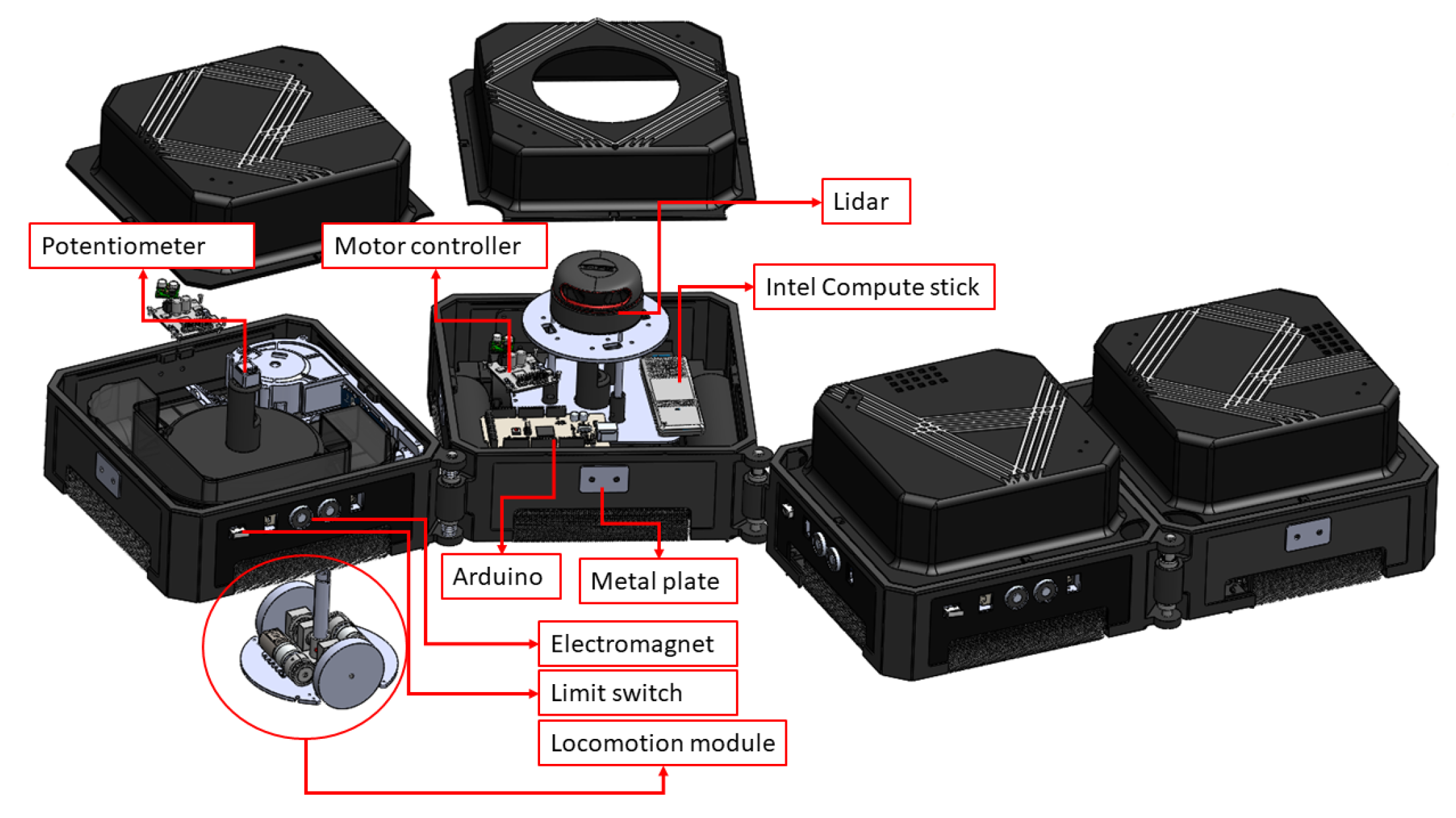
2. hTetro-Reconfigurable Floor Cleaning Robot

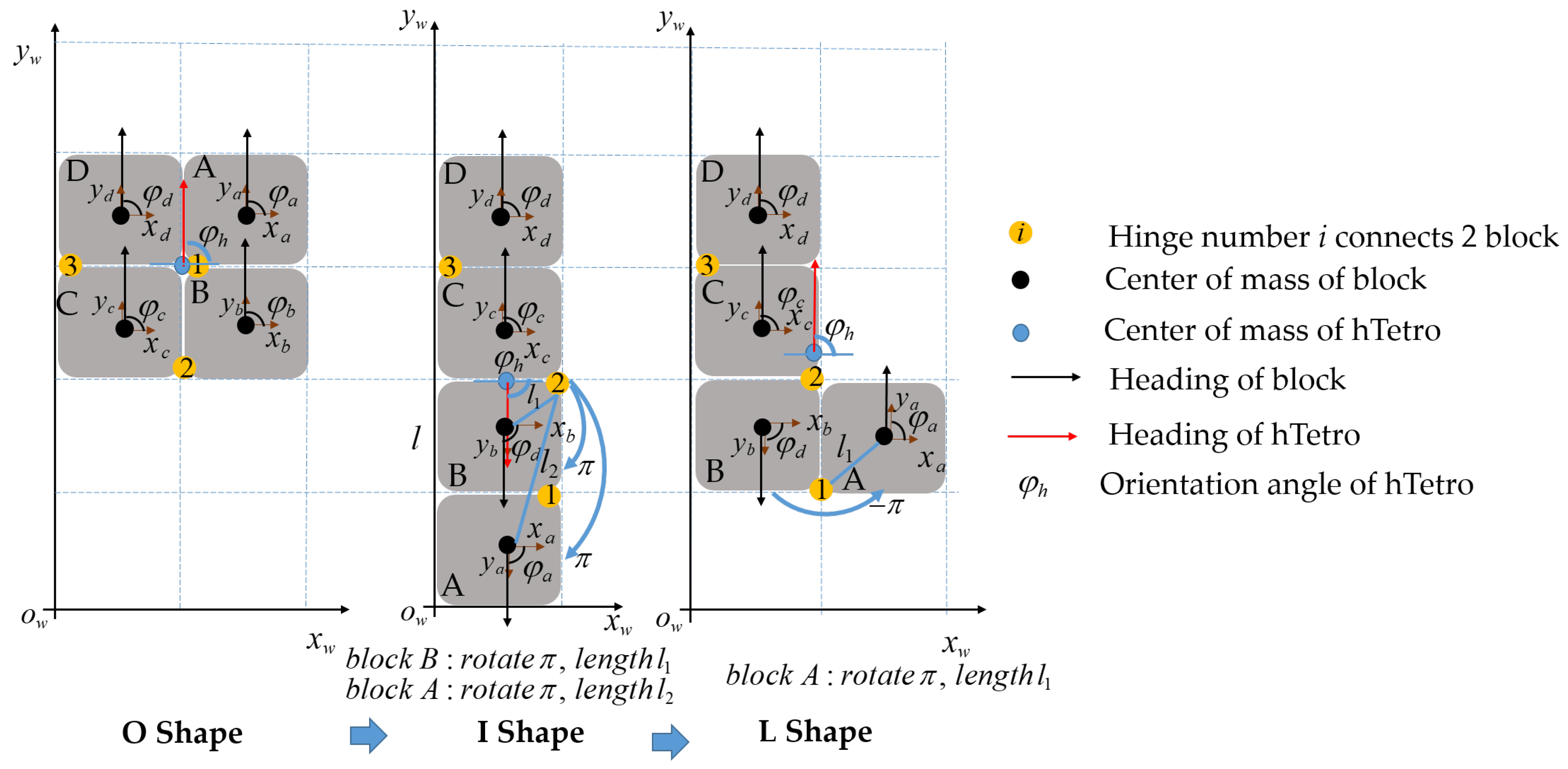
2.1. hTetro Kinematic Design with Differential Drive Mechanism

There are numerous floor cleaning robots in the market but they are all in fixed morphology of circle, space, and oval and struggle to cover the complex environments. In addition, most of the existing reconfigurable robot are not compatible for cleaning purpose due to the dependent locomotion (for instance, locomotion is performed by rolling the platform), cleaning module design (for instance, cleaning modules must be on multiple sides of the platform in case of rolling locomotion) and subsequently the size and capacity of locomotion and cleaning modules. On the other hand, the capability of hTetro to change its shape to seven tetromino morphologies O, Z, L, T, J, S, I and ability to implement the locomotion within each configuration are similar to our previous works of [28]. It is worth noting that in this work which benchmarked the performance of hTetro with fix form robots, we put great emphasis on the robots’ capability of cleaning the entire room without leaving any uncleaned space behind by activating the cleaning modules operate continuously during robot navigation. With the reconfigurable robot design, the polyomino tiling theory [29] improves the navigation strategy by providing guaranteed complete coverage of the space, but it does not change the cleaning action of the hTetro robot. This represents that the robot is still performing continuous cleaning actions during the navigation, which is similar to the currently commercialized household cleaning robots, rather than only activating the cleaning modules when the hTetro robot arrives at the waypoint locations in the tilesets. To this end, this class of robot needs to perform locomotion and transformation tasks smoothly. The locomotion the hTetro robot platform in [28] of each block is being operated by four DC motors attached with omnidirectional wheels, and the transformation to seven tetromino shapes is executed by rotating to defined angles of servo motors at hinges connecting four robot blocs.

In this work, we have developed a new hTetro kinematic architecture which takes into consideration the maneuverability to reduce the complexities and improves the precision of various types of operations including transformation, orientation adjustment, and translation mechanisms. The improved hardware architecture is showed in Figure 1. Specifically, the hTetro platform consist of four flexible mobile blocks indexed A, B, C, D in world frame coordinate w. The four square-shaped hTetro blocks are identical in size and are connected by three hinges, which provide 180-degree freedom of movement between the connected blocks and play a crucial role in the realization of hTetro shape-shifting. A 2D LiDAR, an Intel computer stick, and an Arduino microcontroller are mounted inside block B to enable the autonomous navigation. The hTetro was built with four modules in which the dust bins can be dismantled easily. The dust bins are mounted by snap fit design inside four modules as Figure 1. Although the user has to empty four separated dustbins each time, the number of time that the user frequently clean the dust bins can be reduced by four times if the overall dustbin capacity was increased by four times. In the future, each module of hTetro can execute the cleaning tasks independently and are able to collaborate with other modules to clean large and complex environments. Each block is of length 140 mm, width 140 mm, and 55 mm height and is equipped with a differential drive module as shown in Figure 2, which consists of two 12V DC motors and a central rod. The differential drive modules are connected to the blocks through bushing joints on the central rods, and passive cylindrical joints are used for the connection between two different blocks. The velocities of the wheels determine both transformation and locomotion motions of the unit. By adjusting the speed ratios of different wheels, the hTetro robot is able to traverse linearly in all directions or follow along curves with different curvatures. The steering ability that provided by four differential drives hTetro helps the robot successfully execute three types of action: (1) transformation between different morphologies, (2) translation locomotion to connect waypoints in the workspace, and (3) adjustment of orientation around the center of robot mass (COM) while maintaining its morphology. The operations of these modules all contribute to the energy consumption of the system during the navigation and have to be evaluated independently. One of the advantages of utilizing reconfigurable design instead of a fixed morphology design is that robots with reconfigurability are able to easily access narrow spaces, resulting in better overall coverage of the workspace. The design of a reconfigurable robot also provides the robot with the flexibility to evaluate the energy cost in the workspace and determine the best strategies and series of motions that yield minimum energy consumption.

As the joints between blocks are passive joints, electromagnets on the side walls are used to hold the blocks together during the locomotion, while limit switches are used to determine the end of transformation as well as the configuration status of the unit. The possible heading angles of each block i on the global frame ${\phi }_i=\{0,\frac{\pi }{2},\pi \}$ in both clockwise and anticlockwise direction. By moving a single block individually or two adjacent blocks together, the hTetro can be changed to seven morphologies as in Figure 3. This hTetro operation during implementing complete path planing with the aspects of energy efficiency are concerned in this paper. To this end, the energy consuming by each operation of the robot and the optimal sequence concerning energy efficient will be modeled in the following sections.

2.2. Representation of hTetro in a Workspace

The Figure 4 represents the generalized global coordinates of the hTetro location in the workspace and the shapeshifting progress from O to I then to L shape.

Table 1. Terminologies description for navigation of hTetro on workspace.

Terms	Meaning
$m_i$	Mass of the module i where $i\in \mathbf{H}=\{a,b,c,d\}$
$(x_i^s,y_i^s)$	Center of mass of module i where $i\in \mathbf{H}=\{a,b,c,d\}$ at waypoint s
$(x_h^s,y_h^s)$	Center of the mass of the robot at waypoint s
$(x_h^{s*},y_h^{s*})$	Center of the mass of the robot at waypoint s after transformation
$(x_h^d,y_h^d)$	Center of the mass of the robot at next destination waypoint d
$f_{transl}$	Function to calculate the total distance translated by all modules towards the desired target location
${\theta }_i$	The required angle to perform the transformation by module i where $i\in \mathbf{H}=\{a,b,c,d\}$
$l_1$	Turning radius for the module in Single Module Locomotion (SML)
$l_2$	Turning radius for the outermost module in Double Module Locomotion (DML)
$f_{transf}$	Function to calculate the total distance travelled by all module to perform transformation
$l_i^s$	Magnitude of the distance between center of the mass of each module and that of the robot where $i\in a,b,c,d$ at waypoint s
${\phi }_h^d$	Desired orientation of the robot at waypoint d with respect to the global frame
${\phi }_h^s$	Current orientation of the robot at waypoint s with respect to the global frame
${\phi }_h^{s,d}$	Orientation offset of the robot after tramsfomation from waypoint s to waypoint d as in Table 4
$f_{orient}$	Function to calculate the total distance travelled by all modules towards the desired orientation
$C(W_n^s,W_n^d)$	Total travelled distance for a pair n by the robot from one source waypoint $W^s$ to next destination waypoint $W^d$ performing transformation, translation, orientation correction

are the terminologies defined to describe the hTetro configurations in the global coordinate. To fit the morphologies of hTetro in a specific tileset, reference coordinates of waypoints inside the workspace need to be generated by the CCPP approach. Thus, the center of mass (COM) of hTetro is chosen as the waypoint position. The hTetro frame at waypoint with label s is defined by $\{x_h^s,y_h^s,{\phi }_h^s\}$, which describes the COM of hTetro in each robot morphology. The corresponding frame of each module is defined by $\{x_i^s,y_i^s,{\phi }_i^s\}$, where i represents the block ID $(i\in \mathbf{H}=\{a,b,c,d\left\}\right)$. Please note that the orientation of the robot (${\phi }_h^s$) is set to be identical to the orientation of block A (${\phi }_a^s$). The local navigation procedure between source waypoint $W^s$ and waypoint $W^d$ inside the workspace of the complete path planning is shown in Figure 5. As mentioned previously, there are three main categories of hTetro motions, namely the permutation of transformation, the linear translation, and the orientation adjustment according to the required configuration on the workspace. These motion tasks are the main contributing factors in our cost functions regarding distance traveled and energy consumption. Specifically,

Table 2. Turning angle ${\theta }_i$ of each block when hTtro transforms shape from Source waypoint $W^s$ to next Destination waypoint $W^d$.

	${\mathit{W}}^{\mathit{d}}$	O Shape A B C D	I Shape A B C D	L Shape A B C D	Z Shape A B C D	T Shape A B C D	J Shape A B C D	S Shape A B C D
${\mathit{W}}^{\mathit{s}}$
O Shape		0 0 0 0	$\pi$$\pi$ 0 0	($\pi$,$-\pi$) $\pi$ 0 0	$-\pi$ 0 $-\pi$ ($-\pi$,$-\pi$)	$-\frac{\pi }{2}$ 0 0 $-\pi$	($\frac{\pi }{2}$,$-\pi$) $\frac{\pi }{2}$ 0 $\pi$	($\frac{\pi }{2}$,$-\pi$) $-\frac{\pi }{2}$ 0 0
I Shape		$-\pi$$-\pi$ 0 0	0 0 0 0	$-\pi$ 0 0 0	$-\pi$ 0 0 $-\pi$	$-\frac{\pi }{2}$ 0 $\pi$ ($\pi$,$-\pi$)	($-\frac{\pi }{2}$,$-\pi$) $-\frac{\pi }{2}$ 0 $-\pi$	($-\frac{\pi }{2}$,$-\pi$) $-\frac{\pi }{2}$ 0 0
L Shape		($-\pi$,$\pi$) $-\pi$ 0 0	$\pi$ 0 0 0	0 0 0 0	0 0 0 $-\pi$	$-\frac{\pi }{2}$ 0 $-\pi$ ($\pi$ $-\pi$)	0 0 0 $\pi$	$-\frac{\pi }{2}$$-\frac{\pi }{2}$ 0 0
Z Shape		$\pi$ 0 $\pi$ ($\pi$,$\pi$)	$\pi$ 0 0 $\pi$	0 0 0 $\pi$	0 0 0 0	$\frac{\pi }{2}$ 0 $\pi$ $\pi$	$-\frac{\pi }{2}$$-\frac{\pi }{2}$ 0 0	$-\frac{\pi }{2}$$-\frac{\pi }{2}$ 0 $\pi$
T Shape		$\frac{\pi }{2}$ 0 0 $\pi$	$\frac{\pi }{2}$ 0 $-\pi$ ($-\pi$ $\pi$)	$\frac{\pi }{2}$ 0 $\pi$ $\pi$	$-\frac{\pi }{2}$ 0 $-\pi$ $-\pi$	0 0 0 0	$\frac{\pi }{2}$ 0 $\frac{\pi }{2}$ $\frac{\pi }{2}$	($\frac{\pi }{2}$, $-\frac{\pi }{2}$) $\frac{\pi }{2}$ 0 $\pi$
J Shape		($-\frac{\pi }{2}$,$\pi$) $-\frac{\pi }{2}$ 0 $\pi$	($\frac{\pi }{2}$,$\pi$) $\frac{\pi }{2}$ 0 $\pi$	0 0 0 $-\pi$	$-\frac{\pi }{2}$$-\frac{\pi }{2}$ 0 0	$-\frac{\pi }{2}$ 0 $-\frac{\pi }{2}$ $-\frac{\pi }{2}$	0 0 0 0	0 0 0 $\pi$
S Shape		($-\frac{\pi }{2}$,$\pi$) $\frac{\pi }{2}$ 0 0	($\frac{\pi }{2}$,$\pi$) $\frac{\pi }{2}$ 0 0	$\frac{\pi }{2}$$\frac{\pi }{2}$ 0 0	$-\frac{\pi }{2}$$-\frac{\pi }{2}$ 0 $-\pi$	$-\frac{\pi }{2}$ 0 $-\frac{\pi }{2}$ ($-\pi$,$-\frac{\pi }{2}$)	0 0 0 $-\pi$	0 0 0 0

shows the turning angle ${\theta }_i$ each block needs to rotate and

Table 3. Tuning radius of each block when hTtro transforms its shape from Source waypoint $W^s$ to next Destination waypoint $W^d$.

	${\mathit{W}}^{\mathit{d}}$	O Shape A B C D	I Shape A B C D	L Shape A B C D	Z Shape A B C D	T Shape A B C D	J Shape A B C D	S Shape A B C D
${\mathit{W}}^{\mathit{s}}$
O Shape		0 0 0 0	$l_2$$l_1$ 0 0	($l_1$,$l_2$) $l_1$ 0 0	$l_1$ 0 $l_1$ ($l_2$,$l_1$)	$l_1$ 0 0 $l_1$	($l_2$,$l_1$) $l_1$ 0 $l_1$	($l_2$,$l_1$) $l_1$ 0 0
I Shape		$l_2$$l_1$ 0 0	0 0 0 0	0 0 0 $l_1$	$l_1$ 0 0 $l_1$	$l_1$ 0 $l_1$ ($l_2$,$l_1$)	($l_2$,$l_1$) $l_1$ 0 $l_1$	($l_2$,$l_1$) $l_1$ 0 0
L Shape		($l_1$,$l_2$) $l_1$ 0 0	0 0 0 $l_1$	0 0 0 0	$l_1$ 0 0 0	$l_1$ 0 $l_1$ $l_2$	$l_1$ 0 $l_1$ $l_2$	$l_1$ 0 $l_1$ ($l_2$,$l_1$)
Z shape		$l_1$ 0 $l_1$ ($l_2$,$l_1$)	$l_1$ 0 0 $l_1$	0 0 0 $l_1$	0 0 0 0	$l_1$ 0 $l_1$ $l_2$	$l_1$$l_1$ 0 0	$l_1$$l_1$ 0 $l_1$
T Shape		$l_1$ 0 0 $l_1$	$l_1$ 0 $l_1$ ($l_1$,$l_2$)	$l_1$ 0 $l_1$ $l_2$	($l_1$,$l_1$) 0 $l_1$ $l_2$	0 0 0 0	$l_1$ 0 $l_1$ $l_2$	$l_1$ 0 $l_1$ ($l_2$,$l_1$)
J Shape		($l_2$,$l_1$) $l_1$ 0 $l_1$	($l_2$,$l_1$) $l_1$ 0 $l_1$	$l_1$ 0 $l_1$ $l_2$	$l_1$$l_1$ 0 0	$l_1$ 0 $l_1$ $l_2$	0 0 0 0	0 0 0 $l_1$
S Shape		($l_2$,$l_1$) $l_1$ 0 0	($l_2$,$l_1$) $l_1$ 0 0	$l_1$ 0 $l_1$ ($l_2$,$l_1$)	$l_1$$l_1$ 0 $l_1$	$l_1$ 0 $l_1$ ($l_2$,$l_1$)	0 0 0 $l_1$	0 0 0 0

shows the corresponding turning radius $l_1$ or $l_2$ of each block that shifts hTetro from one form to another. The turning angle of the form is the sum of offset angle of hTetro orientation at destination waypoint ${\phi }_h^d$ and the angle ${\phi }_h^{s^{*}}$ which the robot corrects its orientation angle after transformation as described in Figure 5 and tabulated the values in

Table 4. Orientation offset ${\phi }_h^{s,d}={\phi }_h^{s*}-{\phi }_h^s$ when hTtro transforms its shape from Source waypoint $W^s$ to next Destination waypoint $W^d$.

	${\mathit{W}}^{\mathit{d}}$	O Shape	I Shape	L Shape	Z Shape	T Shape	J Shape	S Shape
${\mathit{W}}^{\mathit{s}}$
O Shape		0	$\pi$	0	$-\pi$	$-\pi /2$	$-\pi /2$	$-\pi /2$
I Shape		$-\pi$	0	$-\pi$	$-\pi$	$-\pi /2$	$-3\pi /2$	$-3\pi /2$
L Shape		0	$\pi$	0	0	$-\pi /2$	0	$-\pi /2$
Z shape		$\pi$	$\pi$	0	0	$\pi /2$	$-\pi /2$	$-\pi /2$
T Shape		$\pi /2$	$\pi /2$	$\pi /2$	$-\pi /2$	0	$\pi /2$	0
J Shape		$-\pi /2$	$3\pi /2$	0	$-\pi /2$	$-v$	0	0
S Shape		$-\pi /2$	$3\pi /2$	$\pi /2$	$-\pi /2$	$-\pi /2$	0	0

. After introducing the kinematic design of a Tetris inspired hinge-based self-reconfigurable robot hTetro with the differential drive mechanism, we focus on proposing a navigation strategy that accomplishes complete path planning in following section.

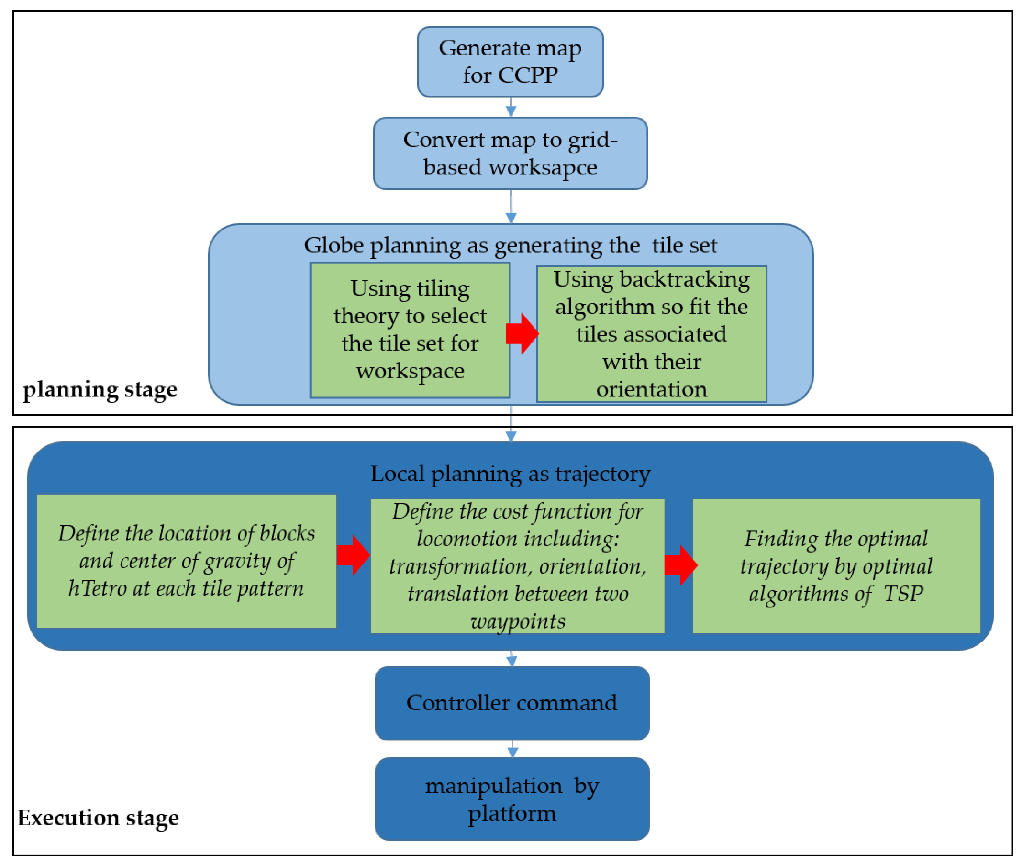
3. CCPP Framework for hTetro by Tilling Theory

The energy consumption during complete coverage the predefined areas of floor cleaning robot is directly related to the navigation trajectory and the series of robot actions, which includes robot transformation, orientation adjustment (clockwise and anticlockwise pivot turn), and linear translation. The complete coverage path planning (CCPP) framework for the hTetro is shown in Figure 6. The process of the proposed framework is divided into two stages. Based on the tiling theory [29,30], the global planning stage focuses on the generation of tileset for predefined grid-based workspace which converted from the captured map. The second stage is the implementation stage, which finding the optimal trajectory called motion planning from the various number of options to connect the generated tileset, then issues the appropriate instruction commands to executes the cleaning and navigation modules to fulfill the complete coverage the workspace. the contribution of the paper by emphasizing the energy estimation model which is based on the hTetro design is highlighted by blocks with italic characters.

The energy consumption optimization approach to the CCPP problem is described as follows. During the planning stage, the polyomino tiling theory [29] provides several lemmas that suggest specific tiling patterns that ensure complete coverage of the predefined workspace. In this paper, the workspace size is segmented into grids in which the workspace has the size of multiple hTetro blocks. The method we have implemented an approximate grid-based decomposition approach as proposed by Choset [15]. Given a random map (works with scenarios where randomly sized furniture and non-parallel wall are presented), this method first decomposes the space into a large grid map, and then it marks any grids where obstacles are presented as “obstacle grids”. Even though it may appear that the workspaces presented in this paper are the “ideal scenarios” where all grids are the same size of hTetro blocks and all obstacles are square-shaped and perfectly aligned with each other, it is a simplified version of the real-world map after approximate cellular decomposition method is implemented. With this workspace modeling method, we could ensure that the proposed optimization strategy is feasible to be implemented in real-world scenarios. Using backtracking algorithm [30], we can estimate the location and orientation of each tetromino pattern of the tileset. This algorithm tries all the possible placements to place one considered tile inside the workspace. When it cannot find the appropriate option for the next tile, it will backtrack to the previous tile and implement the same approach with the new tile among the tileset. The defined workspace can be tiled completely by several tiling set options without any revisited areas. For instance, a 5 × 5 workspace is shown in Figure 7a with the tileset of O, I, L, T hTetro morphologies. The area shaded in red in the workspace depicts the obstacle in the environment which cannot be covered by the hTetro robot. Figure 7b illustrated the position of hTetro blocks and the hTetro robot heading orientation based on the given tileset setting. The specification of robot kinematic design and how robot manipulator modules operate inside the working environment are considered to find the optimal trajectory to complete the found tileset for any specific workspace. During the execution stage, various navigation algorithms are being implemented in order to determine the sequence of these waypoints that minimizes the energy consumption of the entire navigation. As the kinematic control is implemented in the current platform which motion is slow, and the mass is small, we as for now ignored the dynamic part of the platform. Subsequently, the current drawn during acceleration and deceleration is also negligibly small. In addition, we are controlling the quadrature pulse per second (QPPS) of the motor encoder to regulate the desired speed which is only one-third of the motor capacity. Although implementation aspect is simple due to trigonometric equations, the current approach results in the simple and practical solution to approximate the energy consumption in which voltage is regulated and the overall current drawn varies insignificantly during transformation and translations and orientation correction. Thus, energy consumption is directly proportional to the distance traveled, assuming that slippage is negligible which is the case for most mobile robots.

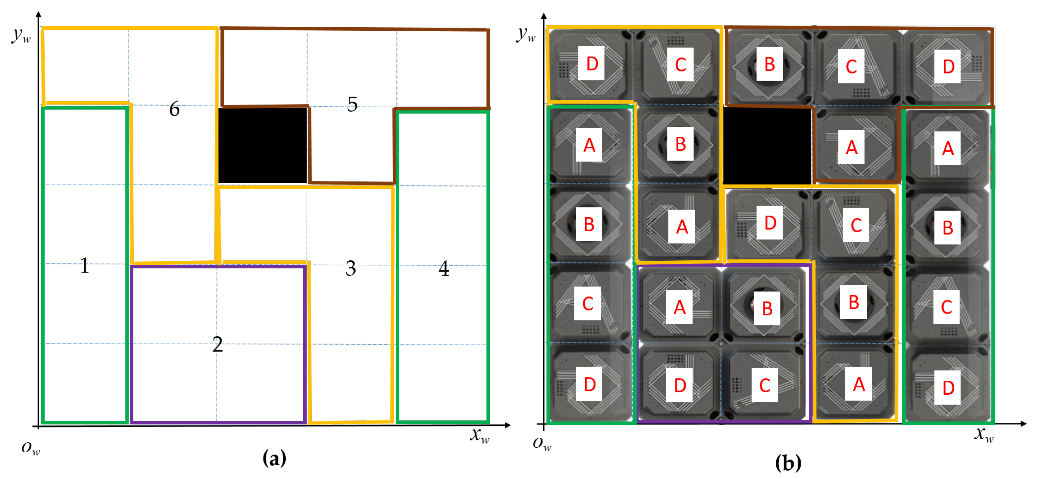
3.1. Localization of hTetro Blocks for Tileset of Workspace

The tileset solution of one workspace only provides the shape and orientation of tetromino patterns. Since the hTetro consists of four linked blocks for one tetromino, block locations robot shape can have several options and these options yield the different navigation energy. The block A, B, C, D order with respective COMs of hTetro for asymmetrical and symmetrical shapes are presented in Figure 8 and Figure 9, respectively. Because of the constraints of hinges locations, there is the option of blocks location for the asymmetrical shape as L, J, T as described in Figure 8. In cases of symmetrical morphologies such as O, I, S, Z, the hinge angles can create several options of blocks locations as shown in Figure 9. Specifically, I, S, Z tiling patterns consist of two options of blocks locations, O tiling pattern consist of four options of blocks locations. Furthermore, the tiling pattern orientation within the workspace is required to locate the block locations. Figure 10 shows the block locations based on the orientation heading of L shape. Algorithm 1 is then applied to assign the optimal block locations from several possibilities of tiling pattern within the workspace w with the size of ($w_r,w_c$) and filled with the proper tileset. In detail, the algorithm follows the row-wise searching to visit each pattern of the tileset. Since there exists only one option of block locations for asymmetric patterns, the blocks locations as shown in Figure 8 are appointed for of an asymmetric tile t. On the other hand, if the considered tile t is in a symmetric shape as shown in Figure 9 which yields similar locations of blocks after hTetro platform executes the transformation, the nearest pattern t − 1 to pattern t is selected. Specifically, Equation (1) can find the block locations on the workspace of symmetrical shapes t with $\mathsf{\Omega }$ options. Please note that Table 2 shows the angles of robot blocks which is required to rotate in order to perform shape transformation. Table 4 provides the orientation offsets of target shapes after the transformations from specific shapes. As a result, the consumed energy for orientation is reduced since the orientation of the form will include the moving of all differential drive units of four blocks and activates all electromagnetic modules. Figure 11 represents the processes of assigning the blocks locations of O shape when the locations of the blocks of previous symmetrical morphology T is known. In this particular case, the block locations of O morphology as in Figure 11a is selected since it yields the same location with the previous T shape orientation.

$$\widehat{t}=\underset{p\in \mathsf{\Omega }}{argmin}\left(\right|{\phi }_h^t-{\phi }_h^{t-1}\left|\right)$$

(1)

Algorithm 1: Finding optimal blocks location for tileset.

1 Function LOCATIONS OF BLOCKS ASSIGNMENT{workspace, tiling set}: 2 workspace{$w(w_r,w_c)$} 3 i ←1, j ←1, t ←1 4    for all i, i ←1, do 5      for all j, j ←1, do 6           if $w(i,j)$ is COM of tiling pattern t then 7                if tiling pattern t is asymmetrical shape then 8                    Assign: blocks locations of t according Figure 8 9                else if t is symmetrical shape then 10                     Do: transformation from tile $t-1$ to tile t (note that orientation of hTetro is defined by Figure 4) 11                     Find: tiling pattern blocks as in Figure 10 which yields the similar location in orientation with the orientation after transformation (note that orientation of hTetro is defined by Table 4) 12                     Assign: blocks locations of t according Figure 9 13              end 14          end 15     end End Function

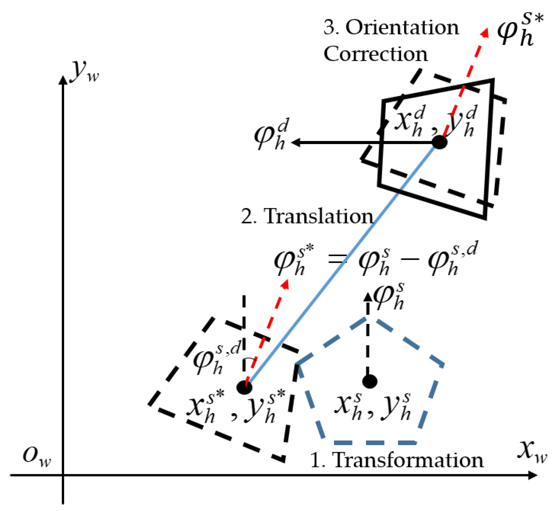
3.2. Local Navigation Weight Function

During the navigation, the hTetro robot follows the defined waypoints and performs a series of actions so that the geometry of hTetro will fit with the tiling patterns without colliding with obstacles in the workspace. We assume that there exists a total of N waypoints in the generated tileset, and each waypoint has a unique label. After using Algorithm 1 to define the locations of the hTetro blocks in the tileset, the 2D locations of the waypoint with label s are denoted as $G(x_h^s,y_h^s)$, which represent the positions of hTetro robot’s center of masses (COM) in the workspace. The position of a COM with respect to the hTetro robot’s local frame can be calculated through Equation (2), which takes into the consideration of the robot mass and relative positions of 4 the hTetro blocks.

$$G(x_h^s,y{}_h^s)=(\frac{{\sum }_{i\in \mathbf{H}}^{}{m}_i{x}_i^s}{{\sum }_{i\in \mathbf{H}}^{}{m}_i},\frac{{\sum }_{i\in \mathbf{H}}^{}{m}_i{y}_i^s}{{\sum }_{i\in \mathbf{H}}^{}{m}_i})$$

(2)

At each location of a waypoint, robot hTetro transforms its shape to the desired shape within tileset by performing single module locomotion or double module locomotion, and then it performs translation motion to travel to the next waypoint before the robot performs the orientation correction to adjust its form to the defined tiling pattern. In this paper, it is assumed that the order of sequence among the three actions of navigation does not affect the final energy consumption during hTetro operations. When a waypoint is cleared, the next waypoint will be updated, and the navigation process is repeated until every pattern within the tileset on the workspace is visited. The entire distance traveled by the differential drive modules in hTetro blocks to accomplish transformation, orientation correction and translation is proportional to the energy consumption of hTetro.

According to Table 3, hTetro blocks are required to either rotate a single module with the turning radius length of $l_1$ or rotate double module with the length of $l_2$ during robot transformation. Assuming that the length of square-shaped hTetro block is defined as l, then $l_1$ and $l_2$ can be derived through Equations (3) and (4), respectively. For instance, in order to perform the transformation from O shape to L shape as demonstrated in Figure 4, module A has to rotate clockwise around hinge 2 for $\pi$ radial with a radius of $l_2$ and then an anticlockwise $-\pi$ radial around hinge 1 with a radius of $l_1$, module B rotates clockwise around hinge 2 an $\pi$ radial with a radius of $l_1$, and modules C, D stay static. In this process, Table 2 is being used to collect the values of $(\pi -\pi )$ $\pi$ 0, while Table 3 is referred to collect the values of $\left(l_1{l}_2\right)$ $l_1$ 0.

$$l_1=\frac{l\sqrt{2}}{2}$$

(3)

$$l_2=\sqrt{{(3l/2)}^2+{(l/2)}^2}$$

(4)

During the navigation process from the source waypoint $W^s$, which is labelled as s, to next destination waypoint $W^d$ labelled as d, the cost function of different hTetro motions are calculated separately. The calculation of transformation cost function is the summation of all blocks’ turning distances, which is the multiplication of absolute ${\theta }_i$ and turning radius of all 4 blocks, as shown in Equation (6). The translation cost function as shown in Equation (7) is the four-time Euclidean distance between the position of COM $(x_h^{s^{*}},y_h^{s^{*}})$ of source waypoint $W^s$ after transformation and the position of COM $(x_h^d,y_h^d)$ of the next destination waypoint $W^d$. Please note that the COM $(x_h^{s^{*}},y_h^{s^{*}})$ can be derived from the blocks locations of hTetro on the workspace coordinate after finishing the transformation to desired destination waypoint $W^d$ morphology as in Equation (2). Finally, the orientation correction cost function is calculated through Equation (8), which is the summation of multiplications of absolute turning angles described in Table 4 and the distances between COMs of each block $l_i^s$ according to Equation (5).

$$l_i^s=\sqrt{{(x_h^s-x_i^s)}^2+{(y_h^s-y_i^s)}^2}$$

(5)

$$f_{transf}(l_1,l_2,{\theta }_i)=\sum _{i\in \mathbf{H}}^{}(l_1+l_2)\left|\left({\theta }_i\right)\right|$$

(6)

$$f_{transl}(x_h^d,y_h^d,x_h^{s^{*}},y_h^{s^{*}})=4\sqrt{{(x_h^d-x_h^{s^{*}})}^2+{(y_h^d-y_h^{d^{*}})}^2}$$

(7)

$$f_{orient}(l_i^s,{\phi }_h^s,{\phi }_h^d)=\sum _{i\in \mathbf{H}}^{}{l}_i^s|{\phi }_h^d-{\phi }_h^{s^{*}}|,\mathrm{where}{\phi }_h^{s^{*}}={\phi }_h^s+{\phi }_h^{s,d}$$

(8)

Assume that a pair ($W_n^s$, $W_n^d$) ($n=1,\dots N-1$) within the trajectory includes the source waypoint $W_n^s$ and the next destination waypoint $W_n^d$, we define the cost between to connect this pair which can be calculated according to Equation (9). In this equation, $\alpha ,\beta ,\lambda$ represents the weight coefficient for transformation, translation, and orientation adjustment, respectively. These coefficients are utilized to adjust the role importance of the three different hTetro actions, and the summation of the three coefficients always equals to 1. A coefficient with larger value represents longer distance traveled and higher energy consumption rate during the associated action. The implementation of weight coefficients is meant to compensate for the inaccuracies from this modeling method, while the exact values of the weight coefficients can be acquired through energy consumption experiments of the physical hTetro robots.

$$C(W_n^s,W_n^d)=\alpha f_{transf}+\beta f_{transl}+\lambda f_{orient}$$

(9)

3.3. Optimization of Trajectory

After assigning the position of hTetro COG called waypoint for each tiling pattern of a typical tileset on a given workspace, the motion planning will produce the sequence connecting these waypoints. The optimal sequence must ensure that the energy consumed to complete this is minimized. There are many possibilities to make a way to connect all the defined waypoints that are already set on the grid-based workspace. Assume that the tileset provides a total of N unsequenced waypoints, and a path describes the directional connection between two waypoints on the map. The CCPP problem can be reformulated as an optimization problem which searches for a trajectory that connects these paths in a way such that every waypoint is visited once throughout the navigation. This optimization problem is a classical Travelling Salesman Problem (TSP), which is considered as NP-hard and unsolvable in polynomial time. A brute force search that iterates through every possible path yields results with factorial time complexity O($n!$), which performs extremely slow when the input size is large. Through Held–Karp algorithm, TSP problems can be solved in O($n^2{2}^n$) time with the aid of dynamic programming [31], but the method still proves to be inefficient in the presented scenario where multiple waypoint patterns are in presence. Therefore, a heuristic-based approach has to be implemented to speed up the calculation time while still providing optimal or near-optimal results.

Here we define the trajectory of hTetro $\eta$ during the navigation as follows: $\eta =\{(W_1^s,W_1^d),(W_2^s,W_2^d)\dots ,(W_N^s,W_N^s)\}$ The hTetro trajectory $\eta$ is a set of directional paths which consists of paths represented as tuples that connect waypoints with two different labels. The trajectory $\eta$ describes the sequence of the waypoints that are being visited: starting from waypoint with the label $W_1^s$ and ending with waypoint with the label $W_N^d$. This trajectory representation is only valid if each waypoint is being visited once. With this definition, the total cost of the trajectory can be calculated as shown in Equation (10). Assume that the ideal trajectory is represented as $\widehat{\eta }$, the ultimate optimization goal of the reformulated CCPP problem is determined through Equation (11) as shown below.

$$C_{total}=\sum _{(W_n^s,W_n^d)\in \eta }^{}C(W_n^s,W_n^d)$$

(10)

$$\widehat{\eta }=\underset{\eta }{\begin{array}{c}\hfill argmin\end{array}}{C}_{total}=\underset{\eta }{\begin{array}{c}\hfill argmin\end{array}}\sum _{(W_n^s,W_n^d)\in \eta }^{}C(W_n^s,W_n^d)$$

(11)

Please note that according to Equation (9), the cost for hTetro to navigate between waypoints with label $W_n^s$ and $W_n^d$ ($C(W_n^s,W_n^d)$) already considers of the distance travelled due to three hTetro actions of navigation: transformation, translation, and orientation adjustment. In this paper, it is assumed that the order of sequence among the three actions of navigation does not affect the final energy consumption during hTetro operations.

In order to find the optimal trajectory $\widehat{\eta }$ and the sequence of waypoints in Equation (11) within a reasonable time, we have managed to implement two types of evolutionary heuristic algorithms to solve the reformulated CCPP problem. Evolutionary algorithms have been widely employed to solve TSP related optimization problems. Each technique has specific mechanisms and representational components that look into nature for inspiration. In this paper, GA and ACO, the two well-known algorithms are taken into consideration. GAs take advantage of the repeating selection and reproduce process to eliminate individuals with under-performing results while maintaining the genetic information from the elites in each generation. The genetic operations such as cross-over and mutations provide GA a wide variety of generated off-springs so that the algorithm does not easily get trapped in local optima. ACO, on the other hand, focus on the probabilistic technique to approach the given problem. By adjusting the ant decisions at the nodes and the constant updates on the pheromones left on each path, the ACO algorithm has proven to be a reliable and consistent strategy to search for the optimal solution of the problem. The work of [25,26] provide additional details on how GA and ACO algorithms were adjusted and implemented to solve TSP. This paper follows similar approaches, which focus on the analysis of the problem, the identification of the crucial components and parameters, and the formulation of the meta-heuristic problems.

The optimization problem in Equation (11) models the energy consumption of the entire navigation process, which consists of adjustable parameters such as the weight coefficients for different hTetro locomotion types. The implementation of heuristic-based algorithms to solve this problem also requires fine-tuning of several heuristic-specific parameters. These parameters are adjusted so that the final result of the calculated energy cost reflects the actual energy consumption in real-world hTetro navigation scenarios with minimal deviation and variation.

4. Experimental Results

There are various precedent algorithms developed to tackle CCPP for the autonomous navigation robots, most of which were evaluated based on the percentage of coverage of the entire environment. In this paper, due to the introduction of hTetro tiling theory and the generated tileset, complete coverage of the entire workspace is guaranteed; therefore, the algorithms implemented to solve the path planning problem focus on the minimization of hTetro power consumption. The two evolutionary algorithms implemented, GA and ACO, are being compared with precedented algorithms such as zigzag, spiral, greedy search, and algorithms introduced in the work of [22], which are all valid approaches to solve TSP-based problems. It is worth noting that algorithms such as zigzag patterned motion are currently the most prominent algorithm that has been implemented in mobile floor cleaning robots. The proposed algorithm was verified in both simulated environment and real-world environment for comparisons. The hTetro block locations and the COMs of waypoints are assigned for tileset through Algorithm 1 and Equation (2). In the first part of the experiment, the results of the simulated environment are provided to show that with the energy function proposed in Equation (9) and the objective function in Equation (11), the proposed algorithm of TSP is capable of finding the optimal trajectory while minimizing total energy consumption. We also compared the results of the proposed method with several GA and ACO parameters setting. In the second part, the generated trajectories of each tested method for workspace 6 × 6 are tested on real robots to evaluate the best performance in terms of energy saving.

4.1. Simulation Environment

The simulated workspaces are being constructed in MATLAB Simulink environment. Each grid cell in the simulated environment corresponds to one block size of the hTetro robot. The workspaces with obstacles and without obstacle are shaped as shown in Figure 12. Specifically, we have chosen the square-shaped workspaces with the size (column × row) of 11 × 11, 8 × 7, and 6 × 6. In this workspace model, a grid cell with a value of $-1$ represents an obstacle, which will be excluded from the generated tileset as the robot must avoid the grid during the navigation. The generated tilesets for simulated workspaces based on polyomino tiling theory [29] and backtracking algorithms [30] are shown in Figure 12. The polyomino tiling theory ensures the predefined workspace is filed entirely by several possible shapes without revisiting grid cells. The appropriate tetromino shapes with orientation are suggested to tile the predefined workspace size by these algorithms. i.e., in Figure 12a the tileset with 9 tetromino morphologies of O, L, J, Z and in Figure 12c the 28 tiling sets of Z, T are selected. The corresponding blocks order (A, B, C, D) and COM for each tile on the workspaces as in Figure 13 are assigned by Algorithm 1 which ensure the next waypoint has the minimum orientation change with the previous waypoint. With the COM waypoint locations within each workspace, the proposed navigation sequence searching algorithm find the trajectory to connect all COM of hTetro tetromino pattern waypoints. The total associated cost calculated by Equation (9) and navigation sequence for each workspace is showed in Figure 13.

Table 5. Comparison results of CCPP methos.

Method	Euclidean Distance	Proposed Cost Weight	Trajectory Generating Time
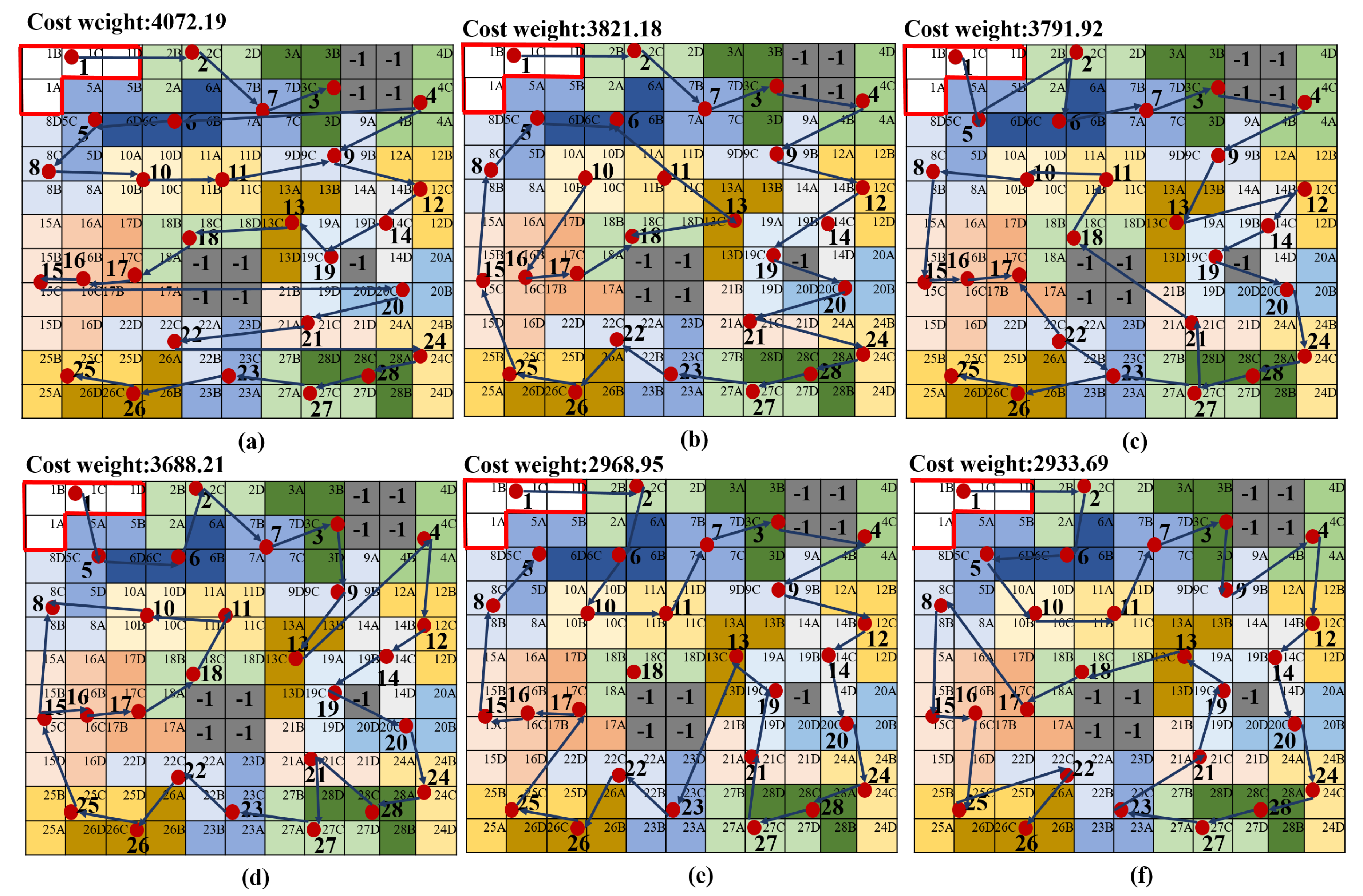
Zigag	3814.12	4072.19	0.012
Sprial	3612.21	3821.18	0.155
Greedy search	2994.52	3791.92	30.24
Method [22]	2943.32	3688.21	1.150
Propsed method GA	3122.56	2968.95	1.158
Propsed method ACO	3125.52	2933.19	1.166

presents the associated cost weights and execution time of several tested CCPP methods including zigzag scanning, spiral scanning, the greedy search, method [22] and the proposed method with GA and ACO for 11 × 11 workspace including 28 waypoints. To conduct the fair comparison, the Table 5 includes both the total cost weight calculated by the total Euclidean distance between waypoint locations which can be considered that only translation action is involved during hTetro navigation and the cost for all three actions transformation, orientation correction and translation calculated by proposed cost function as Equation (9). The zigzag scanning methods connect the waypoints by the one row-wise-nearest searching order. The spiral scanning methods links waypoints by outer to inter searching order. The greedy search optimal trajectories from the starting waypoint to the next nearest waypoint with the lowest associated cost to link all the waypoints. In our previous work [22], the waypoint sequencing problem is formulated as TSP in which the cost value spending to navigate between two waypoints is being formulated under consideration the minimum sum of displacement of the four hTetro robot blocks. As one can observe, the running time of the methods-based TSP is slightly higher than zigzag and spiral methods and considerably lower than the greedy search. Concerning the associated cost weights, the proposed methods can generate the optimal trajectory with the lowest value. In comparison with the method [22], despite yielding the navigation sequence with longer Euclidean distance, the found navigation sequence of the proposed method is different, and its total cost weight calculated by Equation (9) which reflects actual actions during navigation to connect waypoints of hTetro is considerably lower. Typically in Figure 14a with the trajectory sequence of GA and ACO as 1, 3, 2, 7, 9, 6, 4, 5, 8, we can realize these algorithms choice the navigation sequence to connect 2 waypoints with the same morphology first (waypoint 1 to waypoint 3 with the same O shape) instead of link the point at the nearest location (waypoint 1 with O and waypoint 2 with J shape). As the results, the energy associated with the transformation and rotation is reduced, and the number of transformation is minimizing. Please note that these parameters values to derive the optimal results of GA and ACO are selected by applying the trial-and-error method and the best results from the 10 trials are selected to presented in Figure 14 and Table 5.

The effects of coefficient values for deciding the importance of one associated action among transformation, translation, and orientation correction in Equation (9) were analyzed. The

Table 6. Cost weight and trajectory comparison with different coefficients sets for 6 × 6 workspace.

Coefficient Values	Meaning	Cost Weight Action	Cost Weight All Actions	Energy (Ws) on Real Workspace
$\alpha =1,\beta =0,\lambda =0$	Only transformation	1192.35	1239.29	24.32
$\alpha =0,\beta =1,\lambda =0$	Only translation	1198.165	1259.35	25.34
$\alpha =0,\beta =0,\lambda =1$	Only orientation	1201.32	1279.91	28.32
$\alpha =0.5,\beta =0.5,\lambda =0$	transformation and translation	1182.251	1256.80	25.61
$\alpha =0,\beta =0.5,\lambda =0.5$	Only translation and orientation	1198.31	1218.83	24.25
$\alpha =1/3,\beta =1/3,\lambda =1/3$	All three actions	1209.19	1209.19	22.03

and Figure 15 describe results of difference coefficients settings. The different paths with the associated costs are created with coefficient values sets. If we consider the translation motion as the only source that contributes to energy consumption, the cost weight of the path is considerably higher, and the optimal path may vary from the results from other coefficient settings as demonstrated in Figure 15a.

Furthermore, considering specific workspace, the polynomial tiling theory and backtracking can issue several tilesets. Figure 16 provides three different tilesets together with tiling sequence and corresponding cost to cover the grid space of 6 × 6 completely.

Table 7. Cost weight comparison between tiling sets for one workspace.

Workspace	Tiling Set	Cost Weight
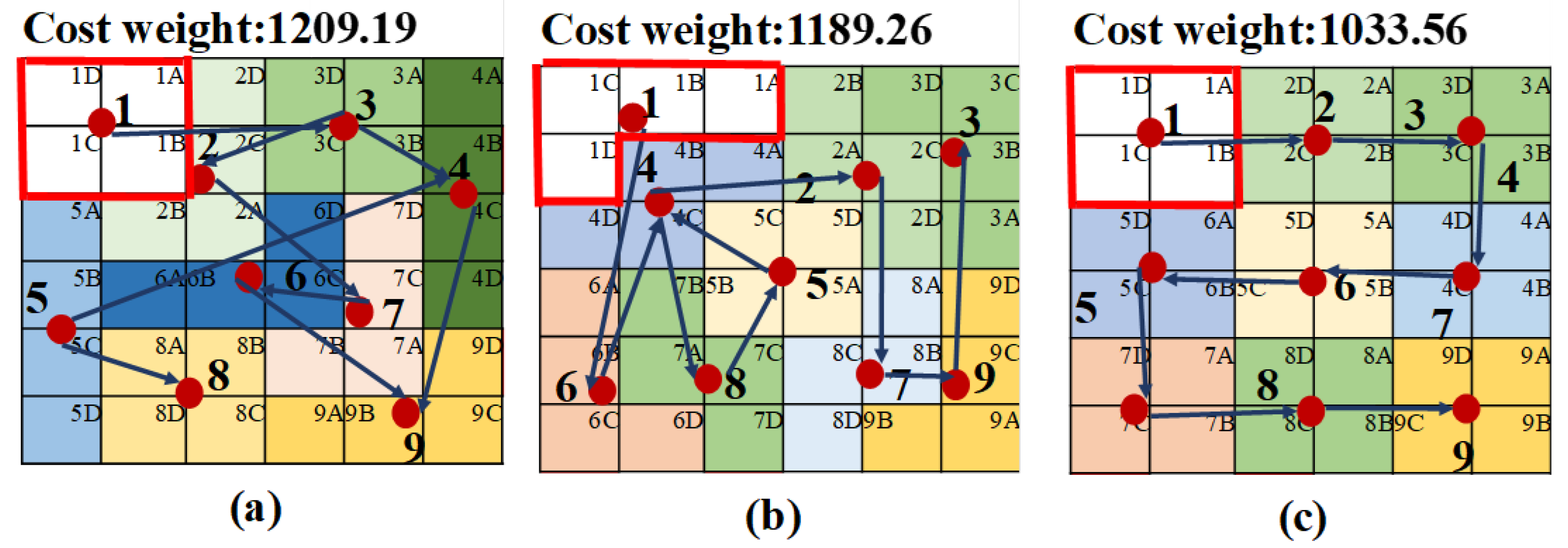
6 × 6	Tileset 1: O, I, J, L	1209.19
	Tileset 2: J, O, L, S, N	1189.26
8 × 7	Tiling set 1: I, L, J	1502.16
	Tileset 2: I, O, L, T	1558.44
11 × 11	Tileset 1: J, T, S, L	2933.69
	Tileset 2: O, I, L, J	2892.68

shows the cost weights for two options of tileset for each tested workspace of Figure 12. Since the proposed CCPP algorithm can provide the optimal trajectories from the suggested tilesets to cover a workspace, the robot can select wisely the optimal tile set that minimizes both time efficiency and energy efficiency. For instance, the O shape can tile the workspace of Figure 12a completely with lowest cost weight trajectory as in Figure 16c. On the other hand, the O has to revisit some grid cells to tile completely Figure 12b and cannot access some grid cells to tile completely Figure 12c with obstacles.

Generally, GA, ACO methods are the meta-heuristic approaches that optimize TSP by gradually enhancing found solutions with better total cost weights. Meta-heuristic based algorithms do not ensure the found solution to be globally optimal; however, the objectives of GA and ACO are to find near-optimal solutions with less iterations and less execution time. In the case of ACO results, the effect of some parameters such as evaporation probability, the number of used ants parameters, on estimating the optimal navigation sequence are studied. On the other hand, this paper also researches parameters that GA outcomes depend on such as the population of the chromosome and mutation probability.

Consider the same 11 × 11 workspace, Table 5 also shows the comparison results of GA and ACO. With parameters of 100 ants agents for each iteration and 0.9 evaporation probability, ACO produces the optimal cost weight, which is 2933.19. While for GA, the optimal cost weight after 100 iterations is 2968.95 by the parameters setting of 0.1 mutation probability and 100 chromosomes. In terms of the length of execution time to achieve these results, GA took a slightly shorter time as compared to ACO.

Table 8. Comparison results of parameters setting for GA.

	Cost Weight	Trajectory Generating Time
chromosome = 30, mutation probability = 0.01	3176.59	1.22
chromosome = 30, mutation probability = 0.05	3371.18	1.31
chromosome = 30, mutation probability = 0.1	3381.32	1.340
chromosome = 100, mutation probability = 0.01	2988.21	1.150
chromosome = 100, mutation probability = 0.05	2998.95	1.662
chromosome = 100, mutation probability = 0.1	2968.95	1.580

shows the cost weights from GA with chromosome population set to 50 and 100, with mutation probability being either 0.01, 0.05, or 0.1. We can observe that with the increasing number of chromosomes, better results can be observed with the trade-off of slightly longer running time, while the mutation probability does not affect much on the results.

Table 9. Comparison results of parameters setting for ACO.

	Cost Weight	Trajectory Generating Time
number of ants = 50, evaporation probability = 0.1	3372.29	1.412
number of ants = 50, evaporation probability = 0.5	3321.68	1.555
number of ants = 50, evaporation probability = 0.9	3211.97	1.740
number of ants = 100, evaporation probability = 0.1	3688.21	1.850
number of ants = 100, evaporation probability = 0.5	2958.95	1.762
number of ants = 100, evaporation probability = 0.9	2933.19	1.660

shows the shortest path for workspace 11 × 11 as shown in Figure 12, which records the cost weights and the running time for different settings of ACO parameters, including the number of ants and the evaporation coefficient. It can be observed that if the number of ant agents is increased, the cost weight is reduced while yielding a significant urge for execution time. On the other hand, the parameter evaporation probability is proportional to the time to get a similar optimal path of specific ant agents. Figure 17 and Figure 18 plot the results of optimal trajectories cost weights by fixing the mutation parameter as 0.02 of GA, and evaporation coefficient as 0.9 of ACO for 10 trials. We can observe that with one generated cost weight value for workspace as Figure 12a and the generated cost weight values for workspace as Figure 12b, the results of workspaces with a few waypoints are similar during both GA and ACO trials. On the other hand, in the case of larger workspaces, such as the 11 × 11 workspace as shown in Figure 12c, the results of the generated optimal trajectories through GA and ACO varied considerably, with the results from ACO being slightly less consistent across the 10 trials compared to GA method.

4.2. Real Environment Testbed

In Part 2, the real testbed environment was arranged as the 6 × 6 size simulated environment of Figure 12a. The real environment is divided into grids, and each of a grid cell has the size of a real hTetro’s block shape. The proposed CCPP with the parameters of chromosome = 100, mutation probability = 0.1 for GA, and number of ants = 100, evaporation probability = 0.9 for ACO yields the tileset solution of Figure 16a. The experiments were conducted by sending remotely the navigation signal through the Bluetooth to Arduino micro-controller to move hTetro to all waypoints of predefined trajectories. Energy consumption of hTetro robot was recorded through current sensors, which monitored the energy consumed by all the motors of differential drive modules during the entire navigation time. The measured current was sampled at a sampling frequency of 20 KHz sampling rate at the voltage of 12 V. The maximum hTetro motors speed for navigation was set to 1500 rpm. While in idle state, all motors of the robot are deactivated, only working electronics components consume energy. The energy consumption by Arduino in this state is small and about 20 mA at 5 V.

We conducted experiments to find the consumed energies for trajectories by different sets of weight coefficients $\alpha ,\beta ,\lambda$ in Equation (9) and added the experimental results to the last column of Table 6. We can observe that with different estimated trajectories by the sets of weight coefficients, the different consumed energies are created. The results showed that the set of coefficients which consider the importance of all the action of transformation, translation, and orientation equally yields the smallest consumed energies. This proves that the proposed energy model which considers all the travel distance to move the robot from one waypoint to another waypoint can estimate creates the optimal trajectory.

The numerical results of consumption power and the workspace traveling time for different CCPP methods are described in

Table 10. Path Planning Performance Table on Real workspace of 6 × 6 size.

Method	Cost Weight	Running Time (s)	Power (W)	Energy (Ws)
Zigzag	1412.35	147.09	0.285	41.92
Spiral	1391.19	146.42	0.257	40.27
Greedy search	1352.19	136.92	0.238	32.59
Method [22]	1301.25	129.87	0.198	25.71
Proposed method GA	1216.59	122.92	0.185	22.74
Proposed method ACO	1209.19	121.04	0.182	22.03

, respectively. We can observe from Table 10 that robot spends smaller energy if it follows the trajectory of the method with the smaller estimated travel distance as cost weight. Specifically, the consumed energy by the zigzag method is the highest value and close behind the zigzag method is the spiral method. Together with the smallest cost weight, our proposed method by ACO and GA gains the advantages with both the smallest average grid coverage time and the lowest energy consumption. It yields about 10 percent lower than the second best method [22]. The

Table 11. Consumed energy to navigate from source to destination waypoints of proposed trajectory Figure 13a.

Transform	O to O	O to J	J to J	J to L	L to L	L to I	I to I	I to O
Navigation sequence	1 to 3	3 to 2	2 to 7	7 to 6	6 to 9	9 to 4	4 to 5	5 to 8
Consumed energy (Ws)	1.82	3.51	2.11	3.16	2.25	3.32	2.31	3.55

provides the energy robot consumes to navigate from one waypoint to another waypoint of trajectory in Figure 13a. The results from this table showed that robot consumes less energy if there are no transformation, small translation distance and small orientation correction required to move from source waypoint to destination waypoint.These results prove that the proposed complete path planning framework which exploits the robot design and optimal algorithms of TSP is a feasible energy-aware CCPP algorithm to be integrated into physical robots in real-world applications.

5. Conclusions

The CCPP with optimal energy usage during navigation of the represented self-reconfigurable hTetro with differential dive locomotion mechanism has been studied in this paper. Quantifying the three actions as linear and angular distances is a simple method we decided to simplify the energy model complexity of the hTetro structure itself, which consists of multiple moving mechanisms to estimate the optimal trajectory. The proposed CCPP framework with two stages including tileset planning and navigation sequencing showed the best performance of the lowest energy consumption and shortest grid coverage time in both simulation and real-time environments. With the proposed framework, other polyomino based shape-shifting robots can exploit effectively to save energy during navigation. We are developing the hTetro to be able to work autonomously in different testbed environments. Once the platform has been constructed, the energy estimation model with different parameters setting will be evaluated to identify the best optimization technique. Implementing cost functions with the optimal order of actions among transformations, orientation and translation is an interesting research topic. The more sophisticated energy consumption model, which considers the transient states of acceleration, deceleration for each robot joint and the adaptive CCPP considering the dynamic obstacles, slippage, and frictions of different surface types for energy saving is also the future work.

References

- Richter, F. Infographic: Let the Robot Do the Cleaning; Statista: Hamburg, Germany, 2017. [Google Scholar]
- Cleaning Robot Market by Type, Product (Floor-Cleaning Robot, Lawn-Cleaning Robot, Pool-Cleaning Robot, Window-Cleaning Robot), Application (Residential, Commercial, Industrial, Healthcare), and Geography—Global Forecast to 2023. 2018. Available online: https://www.marketsandmarkets.com/Market-Reports/cleaning-robot-market-22726569.html (accessed on 3 March 2019).
- Joseph, L.J.; Newton, E.M.; David, M.N.; Paul, E.S. Autonomous Floor Cleaning Robot. U.S. Patent 7,448,113, 11 November 2008. [Google Scholar]
- Yuan, X.; Zhao, C.X.; Tang, Z.M. Lidar scan-matching for mobile robot localization. Inf. Technol. J. 2010, 9, 27–33. [Google Scholar] [CrossRef]
- Hasan, K.M.; Reza, K.J. Path planning algorithm development for autonomous vacuum cleaner robots. In Proceedings of the IEEE 2014 International Conference on Informatics, Electronics & Vision (ICIEV), Dhaka, Bangladesh, 23–24 May 2014; pp. 1–6. [Google Scholar]
- Gao, X.; Li, K.; Wang, Y.; Men, G.; Zhou, D.; Kikuchi, K. A floor cleaning robot using Swedish wheels. In Proceedings of the IEEE International Conference on Robotics and Biomimetics, ROBIO 2007, Sanya, China, 15–18 December 2007; pp. 2069–2073. [Google Scholar]
- Fink, J.; Bauwens, V.; Kaplan, F.; Dillenbourg, P. Living with a vacuum cleaning robot. Int. J. Soc. Robot. 2013, 5, 389–408. [Google Scholar] [CrossRef]
- Galceran, E.; Carreras, M. A survey on coverage path planning for robotics. Robo. Auton. Syst. 2013, 61, 1258–1276. [Google Scholar] [CrossRef]
- Choset, H.; Pignon, P. Coverage path planning: The boustrophedon cellular decomposition. In Proceedings of the International Conference on Field and Service Robotics, Leuven, Belgium, 16–20 May 1998; Springer: London, UK, 1998; pp. 203–209. [Google Scholar]
- Acar, E.U.; Choset, H.; Rizzi, A.A.; Atkar, P.N.; Hull, D. Morse decompositions for coverage tasks. Int. J. Robot. Res. 2002, 21, 331–344. [Google Scholar] [CrossRef]
- Wang, L.; Gao, H.; Cai, Z. Topological mapping and navigation for mobile robots with landmark evaluation. In Proceedings of the 2009 International Conference on Information Engineering and Computer Science, Wuhan, China, 19–20 December 2009; IEEE: Piscataway, NJ, USA, 2009. [Google Scholar] [CrossRef]
- Xu, L. Graph Planning for Environmental Coverage. Ph.D. Thesis, Carnegie Mellon University, Pittsburgh, PA, USA, 2011; p. 135. [Google Scholar]
- Jin, J.; Tang, L. Coverage path planning on three-dimensional terrain for arable farming. J. Field Robot. 2011, 28, 424–440. [Google Scholar] [CrossRef]
- Cheng, P.; Keller, J.; Kumar, V. Time-optimal UAV trajectory planning for 3D urban structure coverage. In Proceedings of the IEEE International Conference on Intelligent Robots and Systems (IROS 2008), Nice, France, 22–26 September 2008; pp. 2750–2757. [Google Scholar]
- Choset, H. Coverage for robotics—A survey of recent results. Annals Math. Artif. Intell. 2001, 31, 113–126. [Google Scholar] [CrossRef]
- Lumelsky, V.J.; Mukhopadhyay, S.; Sun, K. Dynamic path planning in sensor-based terrain acquisition. IEEE Trans. Robot. Autom. 1990, 6, 462–472. [Google Scholar] [CrossRef]
- Zelinsky, A.; Jarvis, R.A.; Byrne, J.; Yuta, S. Planning paths of complete coverage of an unstructured environment by a mobile robot. Proceedings of International Conference on Advanced Robotics, Tokyo, Japan, 8–9 November 1993; Volume 13, pp. 533–538. [Google Scholar]
- Luo, C.; Yang, S.X. A real-time cooperative sweeping strategy for multiple cleaning robots. In Proceedings of the 2002 IEEE International Symposium on Intelligent Control, Vancouver, BC, Canada, 27–30 October 2002; pp. 660–665. [Google Scholar]
- Gabriely, Y.; Rimon, E. Spiral-stc: An on-line coverage algorithm of grid environments by a mobile robot. In Proceedings of the IEEE International Conference on Robotics and Automation (ICRA 2002), Washington, DC, USA, 11–15 May 2002; Volume 1, pp. 954–960. [Google Scholar]
- Yang, S.X.; Luo, C. A neural network approach to complete coverage path planning. IEEE Trans. Syst. Man Cybern. Part B 2004, 34, 718–724. [Google Scholar] [CrossRef]
- Veerajagadheswar, P.; Mohan, E.R.; Pathmakumar, T.; Ayyalusami, V. A tiling-theoretic approach to efficient area coverage in a tetris-inspired floor cleaning robot. IEEE Access 2018, 6, 35260–35271. [Google Scholar] [CrossRef]
- Le, A.; Arunmozhi, M.; Veerajagadheswar, P.; Ku, P.C.; Minh, T.H.; Sivanantham, V.; Mohan, R. Complete path planning for a tetris-inspired self-reconfigurable robot by the genetic algorithm of the traveling salesman problem. Electronics 2018, 7, 344. [Google Scholar] [CrossRef]
- Arkin, E.M.; Fekete, S.P.; Mitchell, J.S. Approximation algorithms for lawn mowing and milling. Comput. Geom. 2000, 17, 25–50. [Google Scholar] [CrossRef]
- Geng, X.; Chen, Z.; Yang, W.; Shi, D.; Zhao, K. Solving the traveling salesman problem based on an adaptive simulated annealing algorithm with greedy search. Appl. Soft Comput. 2011, 11, 3680–3689. [Google Scholar] [CrossRef]
- Larranaga, P.; Kuijpers, C.M.H.; Murga, R.H.; Inza, I.; Dizdarevic, S. Genetic algorithms for the travelling salesman problem: A review of representations and operators. Artif. Intell. Rev. 1999, 13, 129–170. [Google Scholar] [CrossRef]
- Dorigo, M.; Di Caro, G. Ant colony optimization: A new meta-heuristic. In Proceedings of the IEEE 1999 Congress on Evolutionary Computation, CEC 1999, Washington, DC, USA, 6–9 July 1999; Volume 2, pp. 1470–1477. [Google Scholar]
- Thomas, B. Evolutionary Algorithms in Theory and Practice: Evolution Strategies, Evolutionary Programming, Genetic Algorithms; Oxford University Press: Oxford, UK, 1996. [Google Scholar]
- Le, A.; Veerajagadheswar, P.; Sivanantham, V.; Mohan, R. Modified a-star algorithm for efficient coverage path planning in tetris inspired self-reconfigurable robot with integrated laser sensor. Sensors 2018, 18, 2585. [Google Scholar] [CrossRef] [PubMed]
- Conway, J.H.; Lagarias, J.C. Tiling with polyominoes and combinatorial group theory. J. Comb. Theory Ser. A 1990, 53, 183–208. [Google Scholar] [CrossRef]
- A Polyomino Tiling Algorithm. 2018. Available online: https://gfredericks.com/gfrlog/99 (accessed on 3 March 2019).
- Held, M.; Karp, R.M. A dynamic programming approach to sequencing problems. J. Soc. Ind. Appl. Math. 1962, 10, 196–210. [Google Scholar] [CrossRef]