Multi-Labeled Recognition of Distribution System Conditions by a Waveform Feature Learning Model

Abstract

A waveform contains recognizable feature patterns. To extract the features of various equipment disturbance conditions from a waveform, this paper presents a practical model to estimate distribution line (DL) conditions by means of a multi-label extreme learning machine. The motivation for the waveform learning is to develop device-embedded models which are capable of detecting and classifying abnormal operations on the DLs. In waveform analysis, power quality waveform modeling criteria are adopted for pattern classification. Typical disturbance waveforms are applied as class models, and the formula-generated waveform features are compared with field-acquired waveforms for disturbance classification. In particular, filtered symmetrical components of the modified varying window scale are applied for feature extraction. The proposed model interacts suitably with the parameter update method in classifying the waveforms in real network situations. The classification result showed disturbance features on model with the real DL waveform data holds a potential for determining additional DL conditions and improving its classification performance through the update mechanism of the learning machine.

1. Introduction

Power system monitoring and control play an important role in real-time intelligent power distribution networks. In particular, the monitored power signal contains direct operational information and electrical features of the system. It could be further utilized to determine the cause of disturbances in power devices. Power quality (PQ) information is one of the criteria that can be used to measure and evaluate the condition of the distribution system regarding abnormal equipment behaviors and fault conditions [1,2]. In modern distribution lines (DLs) distributed energy resources and bi-directional power sources with grid-tie capabilities may lead to unprecedented operational challenges, the PQ information is believed to be essential in ensuring the high power of networks and preventive management [3,4,5]. In recent years, research in the field of power quality, power system protection and equipment testing has indicated that useful information can be extracted from measured power signal waveforms. An approach for the purpose of equipment health monitoring on DLs by analyzing disturbance waveforms and extracting health status information from them has attracted significant interest from industry and academia [6,7]. In another, waveform signatures and feature extraction have been proposed by using a state prediction approach [8,9].

With respect to waveform data analytics, the primary goal is to extract, from the voltage and current waveforms associated with devices and locations, the signatures of various equipment disturbances and abnormal conditions from which researchers can develop appropriate algorithms to identify equipment abnormalities [10]. However, acquired data in itself is generally insufficient to determine the exact nature of the equipment condition [11]. To extract features from waveform data, disturbance has to be modeled first from the system operation perspective [2,12], and the model’s interaction with the corresponding field device has to be preconceived.

Waveform modeling is used to generate training data for distribution condition classification. In practice, applying the generalized waveform patterns, actual field measured waveforms are compared with and consequently classified for distribution conditions. Some practical solutions developed in recent years [13,14,15] store the waveform data until an PQ event occurs, at which time the particular cycle and sample are detected and compared against the stored waveforms. These methods are restrictively used to allocate diverse signal processing methods such as frequency transformed data compression and sparse signal decomposition [16,17,18].

Application to real-time DL condition recognition and employing end-device condition classifiers are of recent interest. A classifier embedded in feeder devices with improved labeling and waveform modeling could acquire waveforms and recognize abnormal conditions [19,20]. In terms of waveform signal processing, the focuses are on properly extracting waveform signals [21,22], and on waveform signal filtering for exclusion of field waveform noises.

For extraction and classification techniques, the research focuses on an interactive modeling approach to suitably classify the types of PQ disturbances and DL conditions. Also, the approach aims to enable the proposed model to interact with the parameter updating mechanism of learning machines to detect additional unusual waveform disturbance types. As for suggested end-device classification, a modified extreme learning machine (ELM) is adopted and implemented. Several ELM applications have been studied for disturbance waveform classification and fault anticipation [23] due mainly to its superior learning speed and generalization performance which are most desirable for feeder monitoring devices in a small size network [24]. For fixed or variable size networks, with sequential learning and updating, the Online-Sequential ELM (OS-ELM) algorithm has proven generalization performance in several studies and benchmarks involving regression, classification and time-series predictions [25,26]. This study presents and aims to achieve: 1) overcoming the quantity limitation of training waveform data by means of characterized waveform modeling and generation of waveform data from the model; 2) extension to three-phase voltages and currents with digital binary signals from the conventional single-phase classification; and 3) tuning of the model for specific feeder devices to enhance recognition capability for DL condition classification.

2. Modeling the Power Signals and Acquisition Processes

As stated before, the basic structure of the suggested model is, first, to build waveform formula for typical excursions and disturbances which have been frequently observed and, second, to generate the typical waveforms from the formula and maintain a dataset. Then, PQ monitored data are compared with recognized features in the dataset for disturbance identification and classification. Therefore, the proposed learning model setup can be illustrated as in Figure 1, considering multiple data for processing and learning. This section explains the details of each step of the model after a brief description of field data monitoring and collection.

2.1. Field-Measured Waveform Data Processing

As for waveform acquisition as depicted in Figure 1, the waveform types and several update sequence techniques are considered specifically to apply mutual characteristics of the measured signals such as voltage and current, as well as binary values [27]. As to the PQ monitoring, voltage and current measurements in the field devices at monitoring locations are managed by control and operation systems. For the actual network from which the waveforms are acquired, end-point measuring units such as phasor measurement units (PMUs) or feeder remote terminal units (FRTUs), as parts of distribution management systems (DMSs) or power quality management systems (PQMSs), are typically installed, as depicted in Figure 2a,b, respectively.

2.2. Modeling Disturbance Waveforms

There are several mathematical models of PQ waveform generation, see [7,17]. For added generality, the waveform model uses essentially general standard criteria based on the PQ signals and the representative disturbance waveforms referenced by the IEEE-1159-2009 PQ standard [1]. Through consistently modifying the parameters, common PQ disturbances are determined as sag, swell, interruption, flicker, oscillation, notch or impulse transient, spike, and harmonics fluctuations. In addition to these common types, a range-assigned waveform model is applied that is complementarily applicable to abnormal DL condition-related sporadic phenomena. Therefore, the model requires some parameters to be defined in regard to the actual field waveform characteristics; however, the model deals with more comprehensive disturbance features than the conventional PQ criteria.

2.3. Symmetrical Component Processing

Symmetrical components have been used to evaluate unbalanced condition phasors in power system analysis. Their use in waveform analysis is to extract the unbalanced event signals as compared with other phase currents and voltages [7]. Owing to the real-time measurement burdens on the measuring devices, extracting a single phase of the symmetrical value is practiced to reduce the data size. Simultaneity of the disturbance phase is derived as a disturbance trigger condition. Negative sequence components $v_d^{-}(t),i_d^{-}(t)$ are used for the disturbance phase $d\in a,b,c$. These components represent the differences of each phase and return near zero values during steady state, by the implication of which the deviation can be extracted for disturbance recognition from the zero value. The negative sequence component matrix is obtained as follows: as in the frequency domain, the angle can be shifted in the time domain based on the time-dependent variables [28]. This domain change process leads to 1/3 sampling rate for the digital measurement and to normalization once the DL waveform is acquired. The normalization parameter σ^c is determined as:

$${\sigma }_{}^{\mathrm{c}}=\{\begin{array}{cc}1,& \mathrm{modelled}\\ (v_{\mathrm{r}}^{}/{\lambda }_2^{\mathrm{c}})·{\lambda }_{\mathrm{m}}^{\mathrm{c}},& \mathrm{recorded}\end{array}$$

(1)

where $v_{\mathrm{r}}$ represents the rating ratio value; ${\lambda }_2^{\mathrm{c}}$ and ${\lambda }_{\mathrm{m}}^{\mathrm{c}}$ are the secondary value ratio and channel multiplier of Comtrade format waveforms [29], respectively, applied to the recorded DL waveforms. In addition, the sum of negative sequence component $v_t^{abc-}=(v_t^{a-}+v_t^{b-}+v_t^{c-})/3$ is derived as the magnitude of distortions of the saved event. The phase calculation is done with the phase-locked loop (PLL) modulation with real-time phase shifts for the modeling waveforms, and each single waveform will be generated for three phases. For the generation model, disturbance patterns are applied with randomness among one or three phases, depending on the DL condition patterns so that a range of phases is provided randomly to the learning model and the model selectively discriminates the disturbance even though multiple disturbances occur. Despite the fact that the sequence components could be obtained and decomposed, actual samples are usually inseparable by exactly one-third, which causes sequence component noises. The noise is handled by applying an additional filtering method.

2.4. Signal Filtering for Feature Extraction

The noise on measured waveforms has particular measurement errors that occur due to the following causes: one kind is caused by precision errors from the installed field devices of potential and current transformers, which have physical accuracy limitations related to sensor performance. The other is calculation deviations. Even in increased samples for a given measurement cycle, deviations between samples exist because sampling is typically performed in the 3.8 kHz–7.6 kHz frequency range in field devices [29,30]. These errors are distinguishable by tracking the waveform patterns because the majority of the overlapped data is not generally in the steady state. In the negative sequence component, the frequencies are particularly different near the zero region and if the filter is shrunk based on the statistical signal processing method as outlined below, the noise can be eliminated, exposing the remaining waveform features. Noise smoothing has been achieved by generating the cumulative filter using mean and Gaussian values of the negative sequence [31,32].

The negative sequence phase $v_d^{-}(t)$ of ${\mathbf{v}}_{a,b,c}^{-}$ is regarded as the processing signal $s(t)$ in which an unbalance exists. As $s(t)$ has a majority of zero values except for the disturbance, the zero values are not required for the histogram analysis; hence, the signal can be rearranged as ${\mathbf{s}}_{\cancel{0}}$ such that ${\mathbf{s}}_{\cancel{0}}={\mathbf{s}}_t\{s(t)\ne 0\}$ with length $T_{\cancel{0}}$. The histogram bin width uses the square root rule $\mathrm{b}=\lceil \sqrt{T_{\cancel{0}}}\rceil$ or the Sturges method $\mathrm{b}=\lceil 1+{\log }_2(T_{\cancel{0}})\rceil$, which assumes a normal distribution (where the bracket indicates the ceiling function) [33]. From the histogram, the statistics can be modeled by the statistical distribution $p({\mathbf{s}}_{\cancel{0}})$ of a quantified frequency histogram $h({\mathbf{s}}_{\cancel{0}})$ with ${\mathbf{s}}_{\cancel{0}}$ bin levels. The noise can be processed by applying thresholds in which the number of $h({\mathbf{s}}_{\cancel{0}})$ exceeds the expected distribution $p({\mathbf{s}}_{\cancel{0}})$. Gaussian fitting is applied because the signal indicates not only the filtered noise but also the measurement error from the field measuring device. Based on the normal distribution criteria, the upper and lower thresholds of $\underset{\dot{}}{\delta }$ and $\dot{\delta }$ are applied as:

$$\begin{array}{l}\underset{\dot{}}{\delta }=\min \left[{\mathbf{s}}_{\cancel{0}}|h({\mathbf{s}}_{\cancel{0}})>{\omega }_h·p({\mathbf{s}}_{\cancel{0}})\right],\\ \dot{\delta }=\max \left[{\mathbf{s}}_{\cancel{0}}|h({\mathbf{s}}_{\cancel{0}})>{\omega }_h·p({\mathbf{s}}_{\cancel{0}})\right].\end{array}$$

(2)

The method compares two parameters: one represents distribution values and the other numerical counting values. In practical applications, when histogram $h({\mathbf{s}}_{\cancel{0}})$ s frequencies exceed the probability fitting value of $p({\mathbf{s}}_{\cancel{0}})$ with the proper margin weight ${\omega }_h$, the thresholds are applied to the filtering range, starting from the first value to the last exceeded point.

As illustrated in Figure 3, two points that intersect with $h({\mathbf{s}}_{\cancel{0}})$ and $p({\mathbf{s}}_{\cancel{0}})$ are the thresholds for the filter. Consequently, the filtering conditions are sequentially replaced for the obtained waveform’s symmetrical values, and the filtered signal $s_{\mathrm{f}}(t)$ is obtained as follows:

$$s_{\mathrm{f}}(t)\{\begin{array}{ll}s(t)·{\overline{s}}_{\mathrm{st}},& \underset{\dot{}}{\delta }<s(t)<\dot{\delta }\\ s(t),& \mathrm{otherwise}\end{array}$$

(3)

where ${\overline{s}}_{\mathrm{st}}$ is the mean value over the cycle, and the values under the thresholds $\underset{\dot{}}{\delta }$ and $\dot{\delta }$ are filtered as the disturbance samples as indicated in (2). Therefore, as thresholds are determined from the histogram value intersect with the waveform fitted value as described Figure 3 and a mean filter applied for smoothing instead of reducing the values to zero as described for a filtered signal. Because reduction of the sampling error produces better data features for performance and accuracy, this method softens sudden changes in the filtered values. Subsequently, each sample is replaced with the mean value ${\overline{s}}_{\mathrm{st}}$ of its neighboring cycles:

$${\overline{s}}_{\mathrm{st}}=\frac{1}{2·r}{\displaystyle \sum _{t-r}^{t+r}s(t)},\forall t\in T$$

(4)

where, r is the sampling rate per measurement cycle.

2.5. Waveform Representation with Variable Windows

For feature value recognition, fixed size data hardly explains the wavering trend of signal occurrences. Therefore, the feature values are regarded as adjustable information for a progressive data window. In fact, in contrast with the fixed time scale analysis, changing window size has been suggested as a way to enhance disturbance data continuity [5]. Under this variable data window approach, the processed signal $s_{\mathrm{f}}(t)$ is represented as a single vector ${\mathbf{s}}_t=\left[s_1,\cdots ,s_T\right]$, and the cycle separated waveform matrix forms ${\mathbf{s}}_{c,q}$ with sequence control functions as follows:

$${\mathbf{s}}_{c,q}=[s_{c,(c-i_0)·r+(q·i_1)}],\forall c\in C$$

(5)

where c is the cycle number of the entire measurement cycle C; q is the sample sequence ($q=1,\dots ,r$); $i_0$ and $i_1$ are the sequencers controlling the sampling number automatically regarding cycles to window sizes, as defined below, respectively:

$$i_0=\lfloor \ln (q)/\ln (\frac{1}{r})\rfloor ,i_1=\lceil \ln (\frac{q}{r})/\ln (\frac{1}{r})\rceil$$

(6)

To model the variable window, the sample window is set the sample window width w which substitutes c cycle sequences for scalable cycles, and $q=1,\dots ,r_w$. As the adjustable value corresponding to the incrementally sliding window resets, the cycle change does reset shortly after the disturbance is triggered. The extracted value (at the end of the disturbance) is accumulated as the window changes its values. Therefore, the variable window shows both the sustained or momentary waveform continuity signal characteristics that cause the window to expand or contract. With respect to the disturbance duration, the waveform continuity affects the number of extracted cycles, implying that there are fewer windows than normal cycles ($W<C$). Accordingly, sample signal indices are changed to ${\mathbf{s}}_t=[s_1,\cdots ,s_w]$ and the generalized form becomes:

$${\mathbf{s}}_{\begin{array}{l}w,s\\ \end{array}}=[s_{w,(w-i_0)·r_{w-1}+q·i_1}],\forall w\in W$$

(7)

where r_w is the updated sampling window. The variable window ${r_w}^{\infty }$ is determined as $r_w=r·g^{\alpha }$, where $g$ and $\alpha$ denote the base window width and incremental parameter, respectively. As indicated by the window reset condition, the incremental sequence $\alpha$ is derived as follows:

$$\alpha =\{\begin{array}{ll}0& \\ \alpha +1,& \mathrm{if},{\displaystyle {\sum }_{q=1}^{r_w}{s}_{w,q}}\ge \rho \end{array}$$

(8)

where $\rho$ is the trigger value that is the upper limit constant of the filtered value $\left|\delta \right|$ or a pre-determined constant value between 0 and 1. In the study case, 0.1 is applied for the initial trigger condition using measured value averages. Thus, $\alpha$ increases if the cycle average value exceeds the value of $\rho$ for $\forall w$. For instance, for a signal with 40 cycles of sustained disturbances, the window numbers are shortened to six window cycles ($w=[1,2,4,8,16,9]$), from which the parameter $b=2$ is selected. In contrast, a temporary disturbance involves a reset term that is triggered after the disturbance occurs; hence, the sequence is repeated and relatively a larger number of cycles are obtained. As a result, the sample matrix of the variable width signal ${\mathbf{s}}_{w,q}$ is obtained as:

$${\mathbf{s}}_{w,s}=\left[\begin{array}{cccc}{s}_{1,(1-i_0)·r_{w-1}+1·i_1}& s_{1,(1-i_0)·r_{w-1}+2·i_1}& \cdots & s_{1,(1-i_0)·r_{w-1}+r_w·i_1}\\ s_{2,(2-i_0)·r_{w-1}+1·i_1}& s_{2,(2-i_0)·r_{w-1}+2·i_1}& \cdots & s_{2,(2-i_0)·r_{w-1}+r_w·i_1}\\ ⋮& ⋮& \ddots & ⋮\\ s_{W,(W-i_0)·r_{w-1}+1·i_1}& s_{W,(W-i_0)·r_{w-1}+2·i_1}& \cdots & s_{W,(W-i_0)·r_{w-1}+r_w·i_1}\end{array}\right]$$

(9)

2.6. Feature Modeling and Extraction

The sampled waveform is transformed to extract features and the extracted features are used for DL condition classification [34]. Some of basic feature types are derived to measure the grouped features as shown in

Table 1. Feature list of categorized waveforms.

Types	Models
Magnitude (1-norm)	${\mathsf{\Phi }}_n^1={\Vert {\mathbf{s}}_{c,q}\Vert }_1,\forall c,q$
Signal deviation	${\mathsf{\Phi }}_n^2={\displaystyle {\sum }_{w=1}^W{\displaystyle {\sum }_{q=1}^{r_w}{\left(s_{w,q}-{\overline{s}}_w\right)}_{}^2}}$
Disturbance duration	${\mathsf{\Phi }}_n^3={\displaystyle {\sum }_{t=1}^T\left|s_t\right|}/T$
Zero crossing counts	${\mathsf{\Phi }}_n^4={\displaystyle {\sum }_{t=1}^T\left|\mathrm{sign}\left(s_{t-1}\right)-\mathrm{sign}\left(s_t\right)\right|}/C$
Window average	${\mathsf{\Phi }}_n^5={\displaystyle {\sum }_{w=1}^W\left|{\overline{s}}_w\right|}$
Window peak values	${\mathsf{\Phi }}_n^6={\displaystyle {\sum }_{w=1}^W\max ({\mathbf{s}}_w)}$
Window differential	${\mathsf{\Phi }}_n^7={\displaystyle {\sum }_{w=1}^W\left|\mathrm{diff}[\max ({\mathbf{s}}_w)]\right|}$
Cycle RMS a deviation	${\mathsf{\Phi }}_n^8={(s_{\mathrm{rms},c}-{\overline{\mathbf{s}}}_{\mathrm{rms}})}^2$
Peak to RMS	${\mathsf{\Phi }}_n^9=\mathrm{peaktorms}({\mathbf{s}}_{c,q})$
Amplitude of waveforms	$\begin{array}{l}{\mathsf{\Phi }}_n^{10}=\stackrel{·}{\mathrm{statelevel}}[{({\mathbf{s}}_t)}^T]\\ -\underset{·}{\mathrm{statelevel}}[{({\mathbf{s}}_t)}^T],s_t>0\end{array}$

^a Root mean square follows the standard one cycle calculation.

for pattern recognition processes. The features or models are defined as ${\mathsf{\Phi }}_n^{}$ with n = [1, …, N], where the number of data N are for disturbance duration and frequency values. The sustained or the momentary waveform features of the variable window values are selectively calculated corresponding to the types of data in the extraction phase. For the purpose of normalizing data, every feature has relative proportions within 0 and 1.

From Table 1, the norm value ${\mathsf{\Phi }}_n^1$ indicates the magnitude of the measured signal of ${\mathbf{s}}_{c,q}$. In the deviation feature ${\mathsf{\Phi }}_n^2$, ${\overline{s}}_w$ is the mean value obtained from the designated variable window. The duration feature ${\mathsf{\Phi }}_n^3$ is to extract the disturbance sample counts, where $|·|$ is an absolute value. On the other hand, the signal fluctuation count ${\mathsf{\Phi }}_n^4$ measures essential waveform variations. Additionally, for the variable window values, ${\mathsf{\Phi }}_n^5$, ${\mathsf{\Phi }}_n^6$, and ${\mathsf{\Phi }}_n^7$ with their mean, maximum, and differential functions, respectively, extract differences between adjacent samples, and are quantified for window width changes, where “$\max$” is the maximum of the window vector and “$\mathrm{diff}$” is the differential value. Furthermore, additional features are extracted in accordance with the IEEE transitional waveform standard [33]. The modified forms of the features in ${\mathsf{\Phi }}_n^8$, ${\mathsf{\Phi }}_n^9$, and ${\mathsf{\Phi }}_n^{10}$ each having a processing function depending on the waveform characteristics, represent the root mean square (RMS) deviation with $s_{\mathrm{rms},c}=\Vert {\mathbf{s}}_{\mathbf{c}\mathbf{,}\mathbf{s}}{\Vert }_2/\sqrt{r}$ of Euclidian norm, the peak magnitude to RMS value, and the first and second state levels, respectively. In the feature ${\mathsf{\Phi }}_n^{10}$, the state level function which represents the pulse width and jitter trigger as well as the amplitude of the signal suggested particularly in this paper, applies the first and second values to the state level processed values.

3. Learning for Waveform Pattern Recognition

Waveform pattern learning is realized by on-line sequential (OS)-ELM, an improved learning framework. As an extension of ELM, OS-ELM can learn data in consecutive order, block-by-block, to acquire additional waveform data and renew the network [35,36]. For the classification model update, the proposed process uses an empirical model which interacts with field device computing modules on the distribution feeder so that the model can update its network. Flexible and expandability for power distribution phenomena are characteristics of major classification models. Considering the limited resource on the field devices, calculating time on computing unit operations, and updating data size through given commutation environment, ELM is sufficiently capable in which the system tries to use model updates and applications depending on distribution measurement devices.

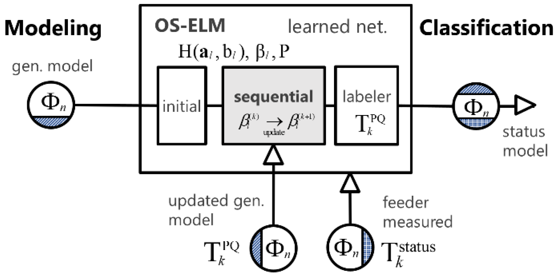
3.1. Using OS-ELM with Condition Signals

As a real-time signal update, OS-ELM is applied for waveform signal learning and re-training. The procedure involving OS-ELM firstly processes the initialization phase and consecutively updates the network with additional blocks of data in the sequential learning phase. For training data $D_k={\{({\mathrm{x}}_n,t_n)|{\mathrm{x}}_n\in {\mathrm{R}}_n,t_n\in {\mathrm{R}}_m\}}_{n=1}^N$, where k is the number of sequences, the pre-determined initial D_o is constrained selectively; and the extracted features of the signal ${\mathrm{x}}_n{=\mathrm{W}}_n·{\mathsf{\Phi }}_n^m$ with the feature weight W_n and t_n are the labeled classes of disturbances. The initial data size implies the hidden node has a certain condition requiring that the rank of the initial network be defined as $N_0\ge L,$ to retain the learning performance in batch ELM [36]. The hidden layer output matrix ${\mathrm{H}}_0$ with the determined $L$ layers in terms of features is modeled as:

$${\mathrm{H}}_0={\left[\begin{array}{lll}G({\mathrm{a}}_1,b_1,{\mathrm{x}}_1)& \cdots & G({\mathrm{a}}_L,b_L,{\mathrm{x}}_1)\\ ⋮& \ddots & ⋮\\ G({\mathrm{a}}_1,b_1,{\mathrm{x}}_{N_0})& \cdots & G({\mathrm{a}}_L,b_L,{\mathrm{x}}_{N_0})\end{array}\right]}_{N_0\times L}$$

(10)

where $G({\mathbf{a}}_l,{\mathbf{b}}_l,{\mathbf{x}}_n)$ denotes the output (activation) function of the l-th hidden node with respect to the randomized network connecting the parameters of the input weights ${\mathbf{a}}_l=\{a_{n,l}{\}}_{n=1,l=1}^{N_0,L}$ and bias ${\mathbf{b}}_l=\{b_l{\}}_{l=1}^L$. The random projection of the hidden network will be unchanged when data in the ${\mathrm{x}}_n$ sequence is updated. From the generalized OS-ELM form, ${\mathrm{H}}_0·{\mathsf{\beta }}_0={\mathrm{T}}_0$, the output $\mathrm{T}({\mathbf{x}}_n|{\mathbf{a}}_l,{\mathbf{b}}_l,{\mathsf{\beta }}_{l,t})$ of transpose ${\mathrm{T}}_0={[d_1,\dots ,d_{N_0}]}_{N_0\times L}^T$ is obtained with regard to a selected output function and the estimated initial output weight ${\mathsf{\beta }}_0=\{{\beta }_{l,t}{\}}^T{}_{l=1,t=1}^L$. Therefore, the minimum function is defined as:

$$\underset{{\beta }_0}{\arg \min }{\Vert {\mathrm{H}}_0·{\mathsf{\beta }}_0-{\mathrm{T}}_0\Vert }_p$$

(11)

where $p$-norm is selected suitably for the minimum function, and the estimated ${\mathsf{\beta }}_0$ values can be obtained by the Moore−Penrose generalized inverse ${\mathrm{H}}^{†}{=(\mathrm{H}}^T·{\mathrm{H})}^{-1}·{\mathrm{H}}^T$ as in [37,38]. Consequently, the initial solution of ${\mathsf{\beta }}_0$ is:

$${\mathsf{\beta }}_0={\mathrm{P}}_0·{\mathrm{H}}^T{}_0·{\mathrm{T}}_0$$

(12)

$$D_{k+1}={\{({\mathrm{x}}_n,{\mathrm{t}}_n)\}}_{n=({\displaystyle {\sum }_{j=0}^k{N}_j)}+1}^{{\displaystyle {\sum }_{j=0}^{k+1}{N}_j}}$$

(13)

where ${\mathrm{P}}_0{=(\mathrm{H}}_0^T·{\mathrm{T}}_0{)}^{-1}$. Following the initialization phase, the sequential learning phase processes the blocks of data using Equation (13) for newly obtained features from the feeder device, with the observation sequence $k=0$ to $k=k+1$ and the number of blocks $N_{k+1}$. Accordingly, the updated partial sequence hidden layer output matrix ${\mathrm{H}}_{k+1}$ is calculated as:

$${\mathrm{H}}_{k+1}={\left[\begin{array}{ccc}G({\mathrm{a}}_1,b_1,{\mathrm{x}}_{({\displaystyle {\sum }_{j=0}^k{N}_j)}+1})& \cdots & G({\mathrm{a}}_L,b_L,{\mathrm{x}}_{({\displaystyle {\sum }_{j=0}^k{N}_j)}+1})\\ ⋮& \ddots & ⋮\\ G({\mathrm{a}}_1,b_1,{\mathrm{x}}_{{\displaystyle {\sum }_{j=0}^{k+1}{N}_j}})& \cdots & G({\mathrm{a}}_L,b_L,{\mathrm{x}}_{{\displaystyle {\sum }_{j=0}^{k+1}{N}_j}})\end{array}\right]}_{N_{k+1}\times L}.$$

(14)

The output target ${\mathrm{T}}_{k+1}={[\begin{array}{ccc}{d}_{({\displaystyle {\sum }_{j=0}^{k+1}{N}_j})+1},& \cdots & d_{{\displaystyle {\sum }_{j=0}^{k+1}{N}_j}}\end{array}]}^T$ is correspondingly achieved to be used in the sequential output weight ${\mathsf{\beta }}_{k+1}^{}$ which is defined as:

$${\mathsf{\beta }}^{(k+1)}={\mathsf{\beta }}^{(k)}+{\mathrm{P}}_{k+1}·{\mathrm{H}}_{k+1}^T({\mathrm{T}}_{k+1}-{\mathrm{H}}_{k+1}^{}·{\mathsf{\beta }}^{(k)})$$

(15)

where ${\mathrm{P}}_{k+1}={\mathrm{P}}_k+{\mathrm{P}}_k·{\mathrm{H}}_{k+1}^T·{({\mathrm{I}+\mathrm{H}}_{k+1}{\mathrm{P}}_k·{\mathrm{H}}_{k+1}^T)}^{-1}·{\mathrm{H}}_{k+1}·{\mathrm{P}}_k$ is obtained by solving the Woodbury matrix inversion formula [39], which avoids calculating the inverse in the recursive process. Because the waveform disturbance trigger is event driven, the model requires a batch data process. In this approach, the process takes the updated model into account and the system gathers the waveforms by the block for OS-ELM.

As shown in Figure 4, after finishing a phase of sequential learning, the model is updated along with its own network settings where training has already been performed. Thus, the renewed model repetitively learns from newer data with the same basis as ELM. The classification model updates its output weight ${\mathsf{\beta }}_{k+1}^{}$ with the pre-determined model setting using the solved ${\mathrm{P}}_{k+1}$ to improve performance. In using the learned model, input-output weights and bias $({\mathbf{a}}_k,{\mathbf{b}}_k,{\mathsf{\beta }}_k)$ are the only required parameters for the feeder device model. Further, to update the model on the feeder devices, the output weights ${\mathsf{\beta }}_{k+1}^{}$ are the only parameters added to the model to be transferred to the devices.

3.2. Condition Classification Model Process

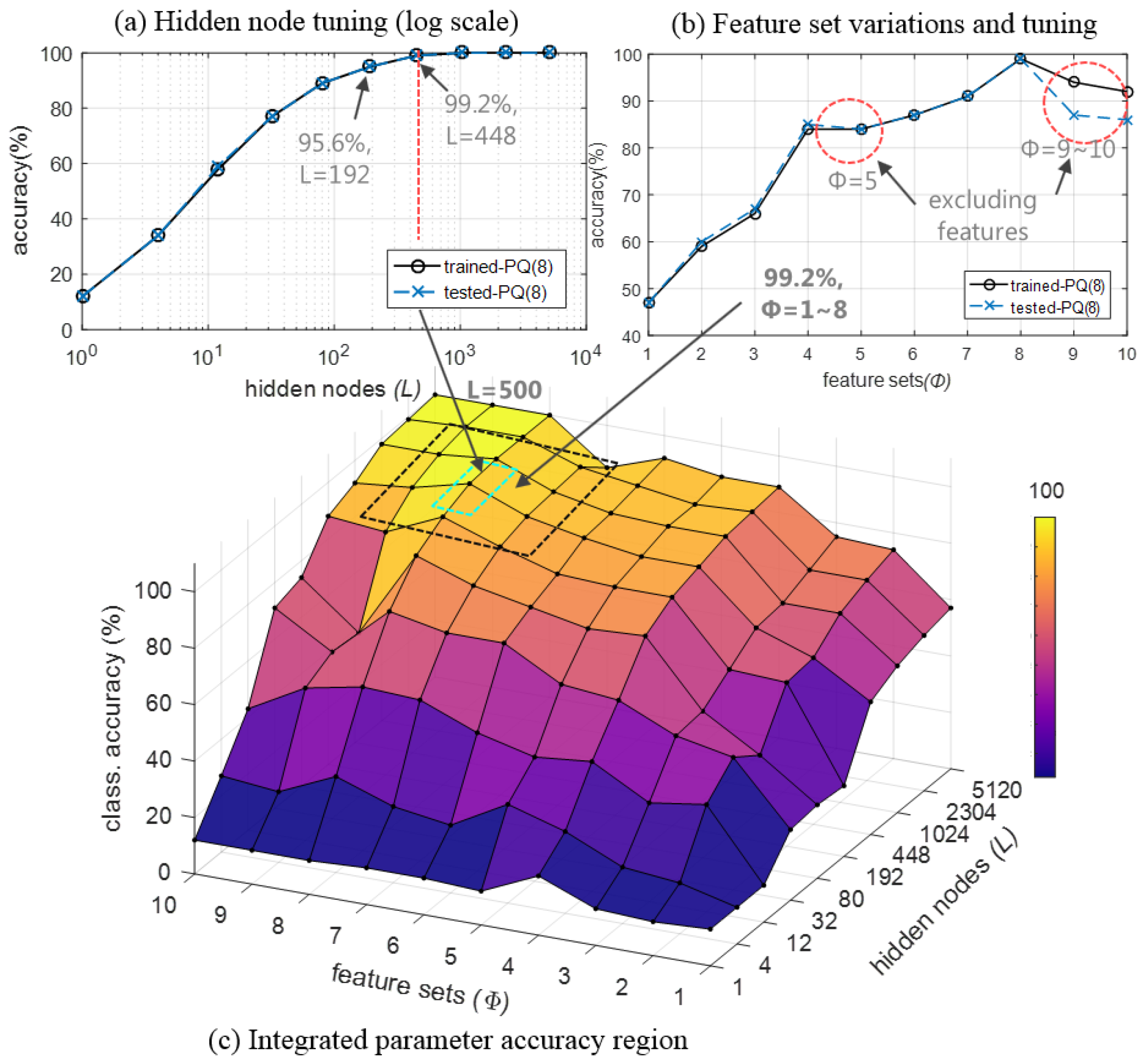
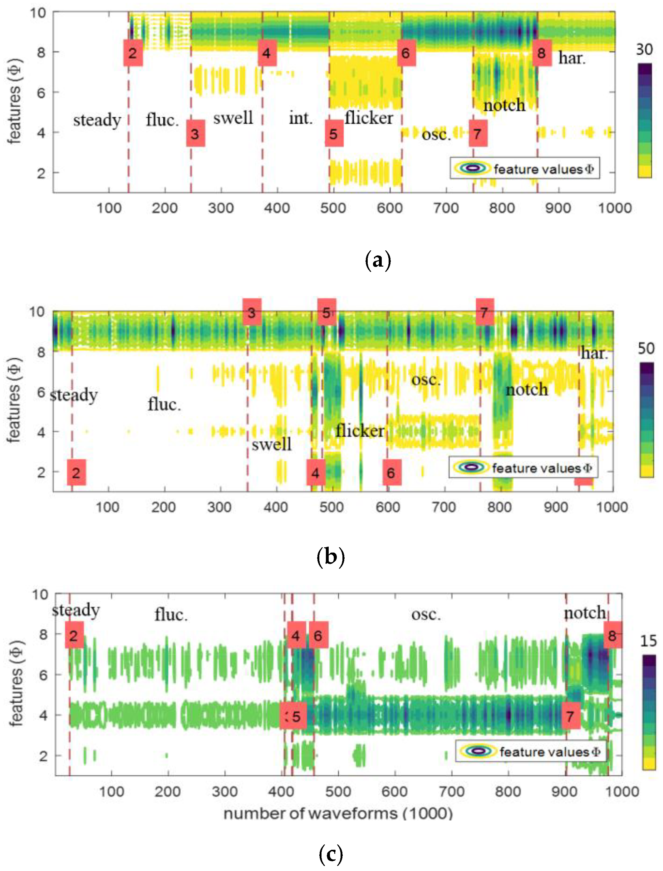
Unlike the single purpose classification ELM, the classification model is regarded as an integrated model that processes multiple DL data including voltage, current, and condition information. It is a multi-labeled classification model that is capable of classifying the feeder measured data and estimating the DL condition.

The process is done in two steps: first, the classification model learns from the modeled condition data and then classifies the field obtained waveforms of the voltages and currents with the condition by the label ${\mathrm{T}}_k^{\mathrm{PQ}}$. In addition, waveforms from the updated model are provided to the sequential learning process after the generation parameters are revised. Second, the model assigns the state label ${\mathrm{T}}_k^{\mathrm{state}}$ to the field obtained data. Thus, the ${\mathrm{T}}_k^{\mathrm{PQ}}$ with the assigned ${\mathrm{T}}_k^{\mathrm{state}}$ are combined. As shown in Figure 5, the initial input condition model-generated data have ${\mathrm{T}}_k^{\mathrm{PQ}}$ only for training; however, the DL measured data and updated sequential model-generated data are then added to the model. When OS-ELM classifies ${\mathrm{T}}_k^{\mathrm{PQ}}$ of the feeder measured waveforms through the label assignment, the output feature includes combined labels of ${\mathrm{T}}_k^{\mathrm{PQ}}$ and ${\mathrm{T}}_k^{\mathrm{state}}$. The resultant labels are delivered to the condition recognition model.

4. Model Validation

The studied model proposes the PQ feature extraction processes with regard to the waveform modeling and field obtained data. For evaluation purposes, waveforms of eight selected types of classes are modeled with the proposed randomized parameters. The voltage and current measurement undergoes the same process as for obtaining the waveform features and each is normalized by the measurement ratings and filters. Because the load change causes voltage distortion in the waveform, each pattern is obtained from the current variation at the same moment.

The field measured waveform was underpinned by C37.111 IEEE Std. [29] so that the voltage and current are properly scaled by the rating values $v_a^{\mathrm{r}}$ and ${\lambda }_2^{\mathrm{c}}$, which were 13.2 to 0.11 on the voltage and 600 to 5 on the current, respectively. The channel multiplier ${\lambda }_{\mathrm{m}}^{\mathrm{c}}$ has a value of 0.00244144 on the FRTU and PQMS measurement units. Symmetrical component $s(t)$ and its filtered value $s_{\mathrm{f}}(t)$ are applied to the feature calculation and are depicted along with $v_{abc}^{-,+}(t),i_{abc}^{-,+}(t)$ of the three-phase negative sequence components.

For other classes of waveform patterns, the learning process involves over 200,000 model-generated waveforms for training, and each block of the sequential input consists of 1000 to 10,000 sets to provide sufficient data and data blocks for adequate learning and accuracy. The hard limit and rectified linear unit (ReLU) activation functions are also selected by examining the model performance iteratively and by applying the cross-validation method. In all validation cases, tuning of $L$ hidden layer nodes, and setting sequence data sets and blocks are determined by the iterative examining process. Furthermore, selective features are analyzed, and if the data sets converged to a certain accuracy level, then the model is deemed to be declared as acceptable.

The tuning process of the hidden nodes and extracted feature sets and trained accuracies as illustrated in Figure 6 demonstrate the range of the adequacy of the model. The number of hidden nodes examined is 200 to 500 as shown in Figure 6a, at the latter of which over 98% classification accuracy is achieved. In terms of the waveform feature sets ${\mathsf{\Phi }}_n^{}$, as shown Figure 6b, some features noticeably contribute to the classification performance, and the features ${\mathsf{\Phi }}_n^{1~4}$ improve average accuracy to 80%. The result indicates that the magnitude features corresponding to the peak and RMS values hold essential information for accurate waveform classification. On the other hand, some inferior feature sets can be observed as the features degrade the performance: accuracy lowers when features ${\mathsf{\Phi }}_n^5$ and ${\mathsf{\Phi }}_n^{9~10}$ are added. To prevent performance degradation, adjustment may be made to the feature weight ${\mathrm{W}}_n$ or the inferior features are removed from the sets.

Figure 7 illustrates the feature regions that are sorted and divided into the classified types for 1000 waveform features. First, the features in Figure 7a, model-generated waveforms and their labels (or classes), show the waveform types evenly with only slight differences and misalignment in set magnitudes and locations between features and classes. On the other hand, classification by field-obtained waveforms of voltage (as shown in Figure 7b and of current (in Figure 7c) has a few erroneous labels (classes). The feature differences between the voltage and current waveform on the same phenomena and their consequential labeling differences are clearly displayed. Therefore, combination of the classifications by both the voltage and current waveforms are adopted for condition recognition in the validation of the suggested model.

Following the example cases explained above, a classification experiment is carried out for the field acquired voltage and current waveforms of the cases of voltage change, fault current, and abnormal trigger.

Table 2. Numbers of classified waveforms regarding acquisition types by FRTUs and PMUs.

Class		1	2	3	4	5	6	7	8
Types		Steady	Fluc.	Swell	Int.	Flicker	Osc.	Notch	Har.	Total
Voltage changes	V	57	620	221	30	164	456	316	115	1979
	I	48	732	27	4	65	953	117	33	1979
Fault currents	V	15	79	40	13	35	190	41	124	537
	I	5	15	24	68	133	79	169	44	537
Abnormal triggers	V	972	2450	140	26	50	548	96	111	4393
	I	123	1658	36	11	125	2339	66	35	4393

displays the outcome of the classification assessment.

Firstly, the voltage change waveforms are classified as fluctuation triggered by the voltage, and as oscillation triggered by the current. The combination of the classification by voltage and current is shown to successfully classify the waveforms into the fluctuation class. Thus, a pair of classes for a certain condition, when combined, provides a new label for recognizing the DL condition, as, for example, the voltage change waveforms are triggered by current pattern variations caused by load changes, sag-swells, and switching operations. Second, for the fault current waveforms cases, the model has brought of three possible classes: oscillation (by voltage) and flicker or notch (by current). Multiple complex faults, fault-clearing actions are of flicker and notch classes. Lastly, the abnormal waveforms have interesting features with multiple triggering conditions capturing unusual patterns compared with the steady state waveforms. Since most of fluctuations and oscillations are triggered by the voltage and current waveforms as the voltage change type, incipient phenomena [40] with small signal variation could be detected in the waveforms, which could be used for anticipating upcoming faults. In summary, the model assessment results indicate a good potential of the developed model for real-network waveform triggers and for embedded classifier for field devices.

5. Discussion and Conclusions

Our method developed a multi-label ELM model for abnormality detection in distribution networks. The study on this discriminating approach has been mainly focused on the signal analytic classification of a single phase or moment in time and no practical application work has been done with complex signals on distribution field. The propose method proves the waveform analytic approach and the machine learning application for the real-time DL state recognition which can help to improve and expand this research area that the studies have not been widely conducted yet. For classifying DL conditions of disturbances in real network, the proposed model is applied to 15,000 field-acquired three-phase voltage and current waveforms, and it is found that the model is highly accurate in classifying DL conditions. Further, the field signals could provide unique patterns for recognition of abnormal operations and fault conditions in the learning mechanism of the classification model. The learned model could necessarily replace the trigger and detection logic on field measuring devices. This affirms the main goal of enabling the classification system to be updated by waveform modeling and feature set reconfiguration using the learning process. The model also found that additional feature sets are needed for furthering performance of the classification model. As applying the condition learning process by patterning the classes form the classification model that proposed, conditional and monitoring classification structures and configurations are significantly important to recognize the DL condition in time-scale and physical connection-based interaction analysis. Even though the model needs to be proved fault or disturbance causation relationships for preventive operation for distribution systems, further studies will combine conventional data and exact labeling together to generate an intelligent classification model for recognizing additional condition types such as intermittently changing conditions.

References

1. 1159-2009—IEEE Recommended Practice for Monitoring Electric Power Quality Industrial and Commercial Applications; IEEE Press: New York, NY, USA, 2009.
2. Gaouda, A.; Kanoun, S.; Salama, M.; Chikhani, A. Pattern recognition applications for power system disturbance classification. IEEE Trans. Power Deliv. 2002, 17, 677–683. [Google Scholar] [CrossRef]
3. Mahela, O.P.; Shaik, A.G.; Gupta, N. A critical review of detection and classification of power quality events. Renew. Sustain. Energy Rev. 2015, 41, 495–505. [Google Scholar] [CrossRef]
4. Santoso, S.; Grady, W.M.; Powers, E.J.; Lamoree, J.; Bhatt, S.C. Characterization of distribution power quality events with Fourier and wavelet transforms. IEEE Trans. Power Deliv. 2000, 15, 247–254. [Google Scholar] [CrossRef]
5. Chakravorti, T.; Patnaik, R.K.; Dash, P.K. Detection and classification of islanding and power quality disturbances in microgrid using hybrid signal processing and data mining techniques. IET Signal Process. 2017, 12, 82–94. [Google Scholar] [CrossRef]
6. Li, B.; Jing, Y.; Xu, W. A Generic Waveform Abnormality Detection Method for Utility Equipment Condition Monitoring. IEEE Trans. Power Deliv. 2017, 32, 162–171. [Google Scholar] [CrossRef]
7. Kumar, R.; Singh, B.; Shahani, D.; Chandra, A.; Al-Haddad, K. Recognition of power-quality disturbances using S-transform-based ANN classifier and rule-based decision tree. IEEE Trans. Ind. Appl. 2015, 51, 1249–1258. [Google Scholar] [CrossRef]
8. Afroni, M.J.; Sutanto, D.; Stirling, D. Analysis of nonstationary power-quality waveforms using iterative Hilbert Huang transform and SAX algorithm. IEEE Trans. Power Deliv. 2013, 28, 2134–2144. [Google Scholar] [CrossRef]
9. Lima, F.P.; Lotufo, A.D.P.; Minussi, C.R. Wavelet-artificial immune system algorithm applied to voltage disturbance diagnosis in electrical distribution systems. IET Gener. Transm. Distrib. 2015, 9, 1104–1111. [Google Scholar] [CrossRef]
10. Martinez-Figueroa, G.D.J.; Morinigo-Sotelo, D.; Zorita-Lamadrid, A.L.; Morales-Velazquez, L.; Romero-Troncoso, R.D.J. FPGA-Based Smart Sensor for Detection and Classification of Power Quality Disturbances Using Higher Order Statistics. IEEE Access 2017, 5, 14259–14274. [Google Scholar] [CrossRef]
11. Santoso, S.; Powers, E.J.; Grady, W.M.; Parsons, A.C. Power quality disturbance waveform recognition using wavelet-based neural classifier. I. Theoretical foundation. IEEE Trans. Power Deliv. 2000, 15, 222–228. [Google Scholar] [CrossRef]
12. Borges, F.A.; Fernandes, R.A.; Silva, I.N.; Silva, C.B. Feature extraction and power quality disturbances classification using smart meters signals. IEEE Trans. Ind. Inform. 2016, 12, 824–833. [Google Scholar] [CrossRef]
13. Liao, C.-C. Enhanced RBF network for recognizing noise-riding power quality events. IEEE Trans. Instrum. Meas. 2010, 59, 1550–1561. [Google Scholar] [CrossRef]
14. Biswal, B.; Biswal, M.; Mishra, S.; Jalaja, R. Automatic classification of power quality events using balanced neural tree. IEEE Trans. Ind. Electron. 2014, 61, 521–530. [Google Scholar] [CrossRef]
15. Dash, P.; Liew, A.; Salama, M.; Mishra, B.; Jena, R. A new approach to identification of transient power quality problems using linear combiners. Electr. Power Syst. Res. 1999, 51, 1–11. [Google Scholar] [CrossRef]
16. Li, J.; Teng, Z.; Tang, Q.; Song, J. Detection and classification of power quality disturbances using double resolution S-transform and DAG-SVMs. IEEE Trans. Instrum. Meas. 2016, 65, 2302–2312. [Google Scholar] [CrossRef]
17. Manikandan, M.S.; Samantaray, S.; Kamwa, I. Detection and classification of power quality disturbances using sparse signal decomposition on hybrid dictionaries. IEEE Trans. Instrum. Meas. 2015, 64, 27–38. [Google Scholar] [CrossRef]
18. Thakur, P.; Singh, A.K. Unbalance voltage sag fault-type characterization algorithm for recorded waveform. IEEE Trans. Power Deliv. 2013, 28, 1007–1014. [Google Scholar] [CrossRef]
19. Rodríguez, A.; Aguado, J.; Martín, F.; López, J.; Muñoz, F.; Ruiz, J. Rule-based classification of power quality disturbances using S-transform. Electr. Power Syst. Res. 2012, 86, 113–121. [Google Scholar] [CrossRef]
20. Ghanbari, T. Kalman filter based incipient fault detection method for underground cables. IET Gener. Transm. Distrib. 2015, 9, 1988–1997. [Google Scholar] [CrossRef]
21. Toscani, S.; Muscas, C.; Pegoraro, P.A. Design and Performance Prediction of Space Vector-Based PMU Algorithms. IEEE Trans. Instrum. Meas. 2017, 66, 394–404. [Google Scholar] [CrossRef]
22. He, H.; Shen, X.; Starzyk, J.A. Power quality disturbances analysis based on EDMRA method. Int. J. Electr. Power Energy Syst. 2009, 31, 258–268. [Google Scholar] [CrossRef]
23. Erişti, H.; Yıldırım, Ö.; Erişti, B.; Demir, Y. Automatic recognition system of underlying causes of power quality disturbances based on S-Transform and Extreme Learning Machine. Int. J. Electr. Power Energy Syst. 2014, 61, 553–562. [Google Scholar] [CrossRef]
24. Li, Y.; Yang, Z. Application of EOS-ELM with Binary Jaya-Based Feature Selection to Real-Time Transient Stability Assessment Using PMU Data. IEEE Access 2017, 5, 23092–23101. [Google Scholar] [CrossRef]
25. Wong, P.K.; Gao, X.H.; Wong, K.I.; Vong, C.M. Online extreme learning machine based modeling and optimization for point-by-point engine calibration. Neurocomputing 2018, 277, 187–197. [Google Scholar] [CrossRef]
26. Wang, B.; Huang, S.; Qiu, J.; Liu, Y.; Wang, G. Parallel online sequential extreme learning machine based on MapReduce. Neurocomputing 2015, 149, 224–232. [Google Scholar] [CrossRef]
27. Negi, S.S.; Kishor, N.; Uhlen, K.; Negi, R. Event Detection and Its Signal Characterization in PMU Data Stream. IEEE Trans. Ind. Inform. 2017, 13, 3108–3118. [Google Scholar] [CrossRef] [Green Version]
28. Paap, G.C. Symmetrical components in the time domain and their application to power network calculations. IEEE Trans. Power Syst. 2000, 15, 522–528. [Google Scholar] [CrossRef] [Green Version]
29. C37.111-1999—IEEE Standard Common Format for Transient Data Exchange (COMTRADE) for Power Systems; Measuring relays and protection equipment—Part 24; International Electrotechnical Commission: Geneva, Switzerland, 1999.
30. Kwon, S.; Kim, J.; Song, I.; Park, Y. Current Development and Future Plan for Smart Distribution Grid in Korea. In Proceedings of the Seminar SmartGrids for Distribution 2008, Frankfurt, Germany, 23–24 June 2008; p. 1. [Google Scholar]
31. De, S.; Debnath, S. Real-time cross-correlation-based technique for detection and classification of power quality disturbances. IET Gener. Transm. Distrib. 2017, 12, 688–695. [Google Scholar] [CrossRef]
32. Singh, U.; Singh, S.N. Detection and classification of power quality disturbances based on time–frequency-scale transform. IET Sci. Meas. Technol. 2017, 11, 802–810. [Google Scholar] [CrossRef]
33. 181-2011—IEEE Standard for Transitions, Pulses, and Related Waveforms (Revision of IEEE Std. 181-2003); IEEE: New York, NY, USA, 2011.
34. Lee, C.-Y.; Shen, Y.-X. Optimal feature selection for power-quality disturbances classification. IEEE Trans. Power Deliv. 2011, 26, 2342–2351. [Google Scholar] [CrossRef]
35. Liang, N.-Y.; Huang, G.-B.; Saratchandran, P.; Sundararajan, N. A fast and accurate online sequential learning algorithm for feedforward networks. IEEE Trans. Neural Netw. 2006, 17, 1411–1423. [Google Scholar] [CrossRef]
36. Lan, Y.; Soh, Y.C.; Huang, G.-B. Ensemble of online sequential extreme learning machine. Neurocomputing 2009, 72, 3391–3395. [Google Scholar] [CrossRef]
37. Huang, G.-B.; Zhu, Q.-Y.; Siew, C.-K. Extreme learning machine: Theory and applications. Neurocomputing 2006, 70, 489–501. [Google Scholar] [CrossRef] [Green Version]
38. Bai, Z.; Huang, G.-B.; Wang, D.; Wang, H.; Westover, M.B. Sparse extreme learning machine for classification. IEEE Trans. Cybern. 2014, 44, 1858–1870. [Google Scholar] [CrossRef]
39. Bishop, C.; Bishop, C.M. Neural Networks for Pattern Recognition; Oxford University Press: Oxford, UK, 1995. [Google Scholar]
40. Kim, C.; Bialek, T.; Awiylika, J. An Initial Investigation for Locating Self-Clearing Faults in Distribution Systems. IEEE Trans. Smart Grid 2013, 4, 1105–1112. [Google Scholar] [CrossRef]
Figure 1. DL waveform feature learning model process.
Energies 12 01115 g001
Figure 2. On-field waveform acquisition devices (sensors). (a) A DL measuring unit location; (b) Feeder remote terminal unit allocations on DLs.
Energies 12 01115 g002
Figure 3. Illustration of the sequence value histogram and applied noise filtering example.
Energies 12 01115 g003
Figure 4. Learning process design for OS-ELM and its update procedure.
Energies 12 01115 g004
Figure 5. Classification network diagram considering learning data sequences.
Energies 12 01115 g005
Figure 6. PQ classification accuracies through parameter changes.
Energies 12 01115 g006
Figure 7. Feature value distributions of classified disturbance types and trigger conditions. (a) Model-generated waveforms; (b) Field obtained voltage waveforms and its classification; (c) Field obtained current waveforms and its classification.
Energies 12 01115 g007