Combustion Optimization for Coal Fired Power Plant Boilers Based on Improved Distributed ELM and Distributed PSO

Abstract

Increasing the combustion efficiency of power plant boilers and reducing pollutant emissions are important for energy conservation and environmental protection. The power plant boiler combustion process is a complex multi-input/multi-output system, with a high degree of nonlinearity and strong coupling characteristics. It is necessary to optimize the boiler combustion model by means of artificial intelligence methods. However, the traditional intelligent algorithms cannot deal effectively with the massive and high dimensional power station data. In this paper, a distributed combustion optimization method for boilers is proposed. The MapReduce programming framework is used to parallelize the proposed algorithm model and improve its ability to deal with big data. An improved distributed extreme learning machine is used to establish the combustion system model aiming at boiler combustion efficiency and NO_x emission. The distributed particle swarm optimization algorithm based on MapReduce is used to optimize the input parameters of boiler combustion model, and weighted coefficient method is used to solve the multi-objective optimization problem (boiler combustion efficiency and NO_x emissions). According to the experimental analysis, the results show that the method can optimize the boiler combustion efficiency and NO_x emissions by combining different weight coefficients as needed.

1. Introduction

Coal-fired power plants have the characteristics of high power, stability, low cost and short construction period, so consequently they occupy a leading position in many countries around the world. However, in the thermal power generation industry, there are a series of problems such as low boiler combustion efficiency and serious pollutant emissions. To improve boiler combustion efficiency and reduce pollutant emissions, the boiler combustion system needs to be optimized.

The use of numerical simulation technology to model coal-fired boilers according to their combustion mechanism and computational fluid dynamic (CFD) is a mature method which is widely used by scholars [1,2]. However, due to the complexity of coal-fired boiler systems, it is often difficult to establish a mathematical model by this method. In recent years, with the continuous improvement of statistical research and the rise of artificial intelligence, support vector machine (SVM) and BP neural network (BPNN) have been widely used in coal-fired boiler modeling [3,4,5]. In these applications, because of the quadratic programming characteristics of support vector machine, it is mainly suitable for small sample data modeling, while BPNN has the shortcomings of easily falling into a local minimum and requiring more human intervention. In 2004, Extreme Learning Machine (ELM) was proposed by Huang, et al. in [6,7] based on generalized Single-hidden Layer Feedforward Networks (SLFNs). ELM can speed up learning by randomly generating input weights and hidden biases and by adopting Moore-Penrose (MP) generalized inversion to determine the output weights. Compared with the traditional gradient-based learning algorithms, ELM not only has faster learning speed and higher generalization performance, but also avoids the difficulties of stopping conditions, learning rate, learning cycle and local minimization encountered by gradient-based learning methods [8]. ELM and its variants [9,10,11] have been applied in many fields [12,13,14], including boiler combustion system modeling [15,16]. Based on the good characteristics of ELM, we choose ELM to model the large number of high-dimensional data of boiler combustion systems.

When using ELM to model a large number of high-dimensional data of a boiler combustion system, the huge memory consumption of matrix calculation destroys the performance of learning algorithm in a single computer environment [17]. The MapReduce programming framework in Hadoop can realize distributed computing of ELM [17,18], thereby improving their computing ability. In this paper, an improved distributed extreme learning machine (IDELM), based on the ELM*I algorithm [19], is proposed to improve the computational efficiency and generalization performance of the algorithm. For pulverized coal-fired boilers, NO_x emissions and boiler combustion efficiency are modeled separately using the proposed IDELM. Two parameters (L and A) in the model are analyzed to select the optimal combination of parameters. Then the two models are combined to build a multi-objective boiler combustion model. Finally, the adjustable input parameters of the boiler combustion model are optimized with the optimized particle swarm optimization (MR-PSO) algorithm to get the optimal combination and use it to guide the boiler combustion system regulation.

The rest of this paper are organized as follows: Section 2 gives a brief review of MapReduce, ELM and the particle swarm optimization (PSO) algorithm. Section 3 provides the implementation of IDELM and evaluates it. Distributed particle swarm optimization (MR-PSO) algorithm is proposed in Section 4. Boiler combustion model based on IDELM algorithm is established in Section 5, and then the specific realization of boiler combustion model optimization in Section 6. Finally, Section 7 presents the conclusions of this paper.

2. Review of MapReduce, ELM and PSO

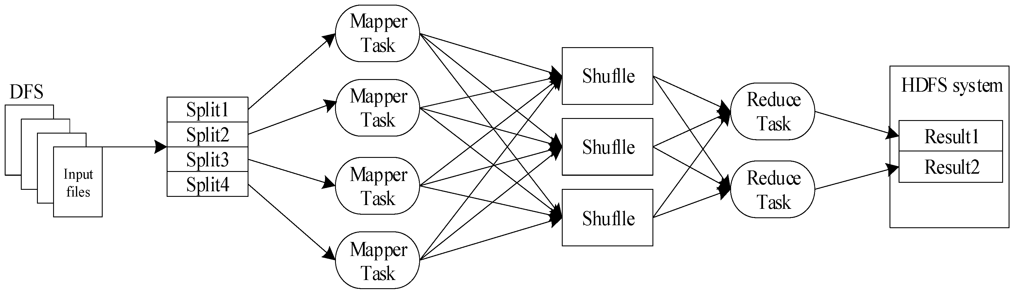
In this section, we describe the methods used in our work, which includes a detailed description of distributed MapReduce framework, then a brief overview of traditional ELM and Ridge Regression Theory to ELM are proposed, finally, the PSO algorithm is introduced.

2.1. MapReduce

MapReduce [20] is a software architecture proposed by Google for parallel computing of large-scale data sets. Its biggest advantage lies in hiding the underlying implementation details of distributed computing. Users do not need to care about the underlying architecture of distributed clusters. They only need to concentrate on the programming of Map and Reduce, which greatly reduces the user’s writing difficulty. In recent years, with the demand of big data processing, MapReduce has gradually become one of the most popular parallel programming models [21,22,23,24].

A typical MapReduce task flow chart is shown in Figure 1. First, the input data is divided into several blocks and stored in the Hadoop Distributed File System (HDFS) [25]. These data is the input to a MapReduce task. Each Map function is assigned a data block, and input as a key-value pair. Then in the Map stage, the MapReduce task allocates a certain number of Mapper tasks. Each Mapper task reads the data block and processes the data according to the user-specified Map function, and outputs the processed set of key-value pairs in the form of another key-value pair result. In the Shuffle stage, a set of irregular key-value pairs output by the Map are merged according to certain rules (for example, merging different values under the same primary key into a list) to make the data have certain rules. In the Reduce stage, the incoming intermediate result list data is sorted or further processed by the user-written Reduce function, and produces the final output of some form of result. Finally, the final data generated by Reduce is written back to the HDFS.

2.2. Extreme Learning Machine

ELM is proposed by Huang e tablet al. [6,7]. Suppose we are training SLFNs with L hidden neurons and activation function g(x) to learn N distinct samples (x_i,t_i), where $x_i={(x_{i1},x_{i2},\cdots ,x_{in})}^{\mathrm{T}}\in R^n$, $t_i={(t_{i1},t_{i2},\cdots ,t_{im})}^{\mathrm{T}}\in R^m$. In ELM, the input weights and hidden biases are randomly generated instead of tuned. Then, the nonlinear system can be converted to a linear system:

$${\displaystyle \sum _{i=1}^L{\beta }_i{g}_i(x_j})={\displaystyle \sum _{i=1}^L{\beta }_{i}g(w_i{x}_j}+b_i)=Y_j,j=1,2,\cdots ,N$$

(1)

where $w_i={({\omega }_{i1},{\omega }_{i2},\cdots ,{\omega }_{in})}^{\mathrm{T}}$ is the weight vector connecting $i-\mathrm{th}$ hidden neuron and input neurons, $b_i$ denotes the bias of $i-\mathrm{th}$ hidden neuron, $w_i{x}_j$ denotes the inner product of $w_i$ and $x_j$, ${\beta }_i={({\beta }_{i1},{\beta }_{i2},\cdots ,{\beta }_{im})}^{\mathrm{T}}$ denotes the weight vector connecting the $j-\mathrm{th}$ hidden neuron and output neurons, $Y_j={(y_{j1},y_{j2},\cdots ,y_{jn})}^{\mathrm{T}}$ is the network output value.

If the actual output of the network equals to the expected output, then ${\displaystyle \sum _{i=1}^L{\beta }_{i}g(w_i{x}_j}+b_i)=t_j,j=1,2,\cdots ,N$, the above equation can be denoted as:

$$H\beta =T$$

(2)

with:

$$H=H({\omega }_1,{\omega }_2,\cdots ,{\omega }_L,b_1,b_2,\cdots ,b_L,x_1,x_2,\cdots ,x_N)=\left[\begin{array}{c}h(x_1)\\ ⋮\\ h(x_N)\end{array}\right]={\left[\begin{array}{ccc}g({\omega }_1\cdot x_1+b_1)& \cdots & g({\omega }_L\cdot x_1+b_L)\\ ⋮& \cdots & ⋮\\ g({\omega }_1\cdot x_N+b_1)& \cdots & g({\omega }_L\cdot x_N+b_L)\end{array}\right]}_{N\times L}$$

(3)

$$\beta ={\left[\begin{array}{l}{\beta }_1{}^{\mathrm{T}}\\ ⋮\\ {\beta }_L{}^{\mathrm{T}}\end{array}\right]}_{L\times m}, T={\left[\begin{array}{l}{t}_1{}^{\mathrm{T}}\\ ⋮\\ t_N{}^{\mathrm{T}}\end{array}\right]}_{N\times \mathrm{m}}$$

(4)

where $H$ is the hidden-layer output matrix, $\beta$ is the output weight matrix, and $T$ is the target output matrix.

According to [7], the output weights is given as:

$$\beta =H^{+}T$$

(5)

where $H^{+}$ is the MP generalized inverse of matrix $H$.

In [9], orthogonal projection method and ridge regression theory are applied to ELM to decompose $H^{+}$. It is pointed out that if $H{H}^{\mathrm{T}}$ is reversible, then $H^{+}=H^{\mathrm{T}}{(H{H}^{\mathrm{T}})}^{-1}$, and if $H^{\mathrm{T}}H$ is reversible, then $H^{+}={\left(H^{\mathrm{T}}H\right)}^{-1}{H}^{\mathrm{T}}$. In the case of a training sample that is not very large, $\beta$ can be expressed as:

$$\beta =H^{\mathrm{T}}{\left(\frac{I}{A}+H{H}^{\mathrm{T}}\right)}^{-1}T$$

(6)

The corresponding ELM output function is:

$$f(x)=h(x)\beta =h(x)H^{\mathrm{T}}{(\frac{I}{A}+H{H}^{\mathrm{T}})}^{-1}T$$

(7)

When the training sample is large, β can be expressed as:

$$\beta ={\left(\frac{I}{A}+H^{\mathrm{T}}H\right)}^{-1}{H}^{\mathrm{T}}T$$

(8)

Then, the ELM output function is:

$$f(x)=h(x)\beta =h(x){(\frac{I}{A}+H^{\mathrm{T}}H)}^{-1}{H}^{\mathrm{T}}T$$

(9)

The term $1/A$ in the formula is a small non-negative number added to the diagonal of $H{H}^{\mathrm{T}}$ or $H^{\mathrm{T}}H$ matrix according to ridge regression theory, which makes the calculation more stable and has better generalization performance [9].

2.3. Particle Swarm Optimization Algorithm

Particle swarm optimization (PSO) algorithm is a swarm intelligence optimization algorithm, which is an algorithm proposed by Kennedy and Eberhart [26] in 1995 inspired by Reynolds’ bird group model theory. In 1998, Shi et al. [27] introduced the inertia weight in the original PSO, which was later called the standard PSO algorithm.

The mathematical model of PSO can be described as follows: Suppose there exists a $D$ dimensional solution in the search space $\Omega$. The number of particles in a particle swarm is n, and each particle has a velocity vector and a position vector. The position of the $i-\mathrm{th}$ particle is $x_i=\left(x_{i1},x_{i2},\dots ,x_{iD}\right)$, the velocity of the $i-\mathrm{th}$ particle is $v_i=\left(v_{i1},v_{i2},\dots ,v_{iD}\right)$, After iterating until the best position of the $i-\mathrm{th}$ particle is $p_{bes{t}_i}^t=\left(p_{i1},p_{i2},\dots ,p_{iD}\right)$, this is called the individual best solution of the particle; the best position found in all the particles is $g_{best}^t=\left(p_{g1},p_{g2},\dots ,p_{gD}\right)$, which is known as the global optimal particle. The PSO algorithm is randomly initialized according to uniform distribution. Then each particle is updated iteratively according to equations (10) and (11). When the convergence condition is satisfied, the update of velocity and position is stopped and the global optimal solution is output:

$$v_i^{t+1}=w_i^t{v}_i^t+c_1{r}_1(P_{Bes{t}_i}^t-x_i^t)+c_2{r}_2(g_{Best}^t-x_i^t)$$

(10)

$$x_i^{t+1}=x_i^t+v_i^{t+1}$$

(11)

where $i=1,2,\dots ,n$, $w_i^t$ is the inertia weight of the $i-\mathrm{th}$ particle velocity; $v_i^t$ is the velocity after the $t-th$ iteration of particle $i$; $c_1$ and $c_2$ are accelerating factors, and the general value is $c_1=c_2=2$; $r_1$, $r_2$ are random numbers uniformly distributed in the [0, 1] interval; $(P_{bes{t}_i}^t-x_i^t)$ is self-learning vectors and $(g_{best}^t-x_i^t)$ is social learning vector. $w$ in the formula uses a linear reduction scheme proposed in literature [27], the specific formula is as follows:

$$w_i^t=w_{\max }-t\frac{w_{\max }-w_{\min }}{ite{r}_{\max }}$$

(12)

where $w_i^t$ is the weight of particle $i$ in iteration $t$; $w_{\max }$ is the maximum value of inertia weight, usually taken as 0.9; $w_{\min }$ is the minimum value of inertia weight, usually taken as 0.4; $ite{r}_{\max }$ is the preset maximum number of iterations; $t$ is the current iteration number.

3. Improved Distributed Extreme Learning Machine (IDELM) Algorithm

In this section, the theoretical basis of our work are firstly introduced. Then, the calculation details of the proposed IDELM are given. Finally, the performance of IDELM is evaluated.

3.1. Preliminaries

In this paper, we use large sample of data to train ELM, so the number of training samples is much larger than the number of hidden layer nodes, namely $N\gg L$. Therefore, $H{H}^{\mathrm{T}}$ is bound to be a large matrix, so that calculating $H{H}^{\mathrm{T}}$ requires consuming a large amount of memory and calculating time. In the worst case, memory may be insufficient. However, the dimensionality of the matrix $H^{\mathrm{T}}H$ is much smaller than that of the $H{H}^{\mathrm{T}}$, so the Formula (8) is more suitable for calculating the output weight $\beta$ of the ELM. To implement the ELM algorithm in the MapReduce framework, we need to find out the parts that can be processed in parallel.

Let $S=H^{\mathrm{T}}H$, $D=H^{\mathrm{T}}T$, then:

$$\beta ={(\frac{I}{A}+S)}^{-1}D$$

(13)

According to Equation (3), there are $h_{ij}=g(w_j\cdot x_i+b_j)$ and $h_{ij}{}^{\mathrm{T}}=h_{ji}=g(w_i\cdot x_j+b_i)$. Then according to the matrix multiplication law, it can be obtained:

$$s_{ij}={\displaystyle \sum _{r=1}^N{h}_{ir}^{\mathrm{T}}}{h}_{rj}={\displaystyle \sum _{r=1}^N{h}_{ri}{h}_{rj}}={\displaystyle \sum _{r=1}^{N}g(w_i\cdot x_r+b_i)}g(w_j\cdot x_r+b_j)$$

(14)

$$d_{ij}={\displaystyle \sum _{r=1}^N{h}_{ir}^{\mathrm{T}}}{t}_{rj}={\displaystyle \sum _{r=1}^N{h}_{ri}{t}_{rj}}={\displaystyle \sum _{r=1}^{N}g(w_i\cdot x_r+b_i)}{t}_{rj}$$

(15)

where $h_{ri}$ is the $i-\mathrm{th}$ element of the $r-\mathrm{th}$ row of the matrix $H$, and $h_{rj}$ is the $j-\mathrm{th}$ element of the same line.

In Equation (13), the elements in the matrix $S$ can be expressed as the sum of the products of $h_{ri}$ and $h_{rj}$. It can be seen that, $h_{ri}$ and $h_{rj}$ are all from the $r-\mathrm{th}$ row of $h_r$, and $h_r$ is the hidden layer output matrix computed by the same group of training input data $x_r$, independent of the other groups of training data. Similarly, $h_r$ and $t_r$ in the formula are also independent of training data from other groups. From the above two equations shows that $S$ and $D$ calculation process is decomposable, so we can make full use of MapReduce parallel framework to achieve $S$ and $D$ calculations. Which can get rid of the shackles of computing and storage capabilities in a stand-alone environment and enable ELM to efficiently train large-scale training data.

3.2. IDELM

According to the above analysis, we know that the process of calculating matrices S and D can be realized by the MapReduce framework, which is an efficient realization to cope with massive training data.

In [19], the ELM*I algorithm implements the calculation of matrix S and D in the MapReduce framework. The solution of the matrix S and D in the Mapper class is partially accumulated. And, to a certain extent, the ELM*I algorithm reduces the calculation, storage and transmission costs of the entire matrix solution. Although ELM*I algorithm performs a partial summation of the solution to the matrices S and D, there is still too much computation time for the program to run on the data extraction and storage. The map and reduce methods used by the original MapReduce framework in Hadoop are executed once for each key-value pair. Generally, there are $N$ key-value pairs for $N$ samples, so the map and reduce methods are executed $N$ times, input and output between the serious increase of the algorithm’s calculation time. The ELM*I algorithm is implemented to the original map and reduce methods. In order to further reduce the transmission and storage cost of the intermediate operation result, the original MapReduce framework needs to be jumped out to reduce the time for transmitting and storing the operation result each time. In order to overcome the shortcomings of ELM*I algorithm, this paper improves the Map and Reduce methods in the Mapper and Reduce classes. Making them execute only one Map or Reduce method for each Map or Reduce task, and storing the intermediate result in HDFS. Finally, using the improved map and reduce methods to calculate the matrix S and D, an improved distributed extreme learning machine (IDELM) is proposed. The specific algorithm steps are shown in Algorithm 1.

Algorithm 1: Improved Distributed ELM (IDELM) S and D calculation steps

1 class SandD

2   // INITIALIZE

3   int L, m

4   s = new ASSOCIATIVEARRAY

5   d = new ASSOCIATIVEARRAY

6  class Mapper

7    h = new ASSOCIATIVEARRAY

8    x = new ASSOCIATIVEARRAY

9    map(context)

10      while (context.nextKeyValue)

11       (x,t) = Parse(contest)

12        for i = 1 to L do

13         h[i] = g(wi ∙x + bi)

14        for i = 1 to L do

15         for j = 1 to L do

16          s[i][j] = s[i][j] + h[i]∙h[j]

17         for i = 1 to m do

18          d[i][j] = d[i][j] + h[i]∙t

19      for i = 1 to L do

20       for j = 1 to L do

21        context.write(triple (‘S’, i, j), s[i, j])

22       for j = 1 to m do

23        context.write(triple (‘D’, i, j),d[i, j])

24   method run(context)

25     map(context)

26  class Reduce

27    reduce(context)

28       while (context.nextKey())

29        sd = 0

30        for (val : values)

31         sd+=val.get()

32       context.write(key, sd)

33   method run(context)

34       reduce(context)

Algorithm 1 contains a main class, which in turn contains the Mapper and Reduce classes. The specific implementation steps of the algorithm 1 can be summarized as follows:

Step 1:

Initialize the number of hidden layer nodes $L$, label $m$, two arrays $s$ and $d$, which are used to store the calculation results of the elements in matrix $S$ and $D$ (Lines 3–5);

Step 2:

In class Mapper, initialize the local variables $h$ and $x$ (Lines 6–8);

Step 3:

In the map method, we first use a while loop to read a sample, and then divide the sample into training data $x$ and the corresponding training result $t$. The separated training sample attribute value $x$ is brought into the partial result $h$ of the loop computation matrix $H$. According to the solved $h$ value and Formulas (14) and (15), the partial accumulation of elements in matrices $S$ and $D$ is calculated, respectively, and the final results are stored in the array $s$ and $d$. The role of the while loop is that when all the <key, value> key pairs in the data block are run, the final sum is stored in $s$ and $d$ (Lines 9–18);

Step 4:

Put s and d in the form of key-value pairs in HDFS (Lines 19–23);

Step 5:

The run method in the Mapper class is overloaded (Lines 24–25);

Step 6:

The reduce method uses a while loop to extract a sample and then initialize a temporary variable. Merge the intermediate results with the same key values in different Mapper to obtain the final accumulated sum of the elements corresponding to the key value (Lines 27–31);

Step 7:

Store the result in HDFS (Line 32);

Step 8:

The run method in the Reduce class is overloaded (Lines 33–34).

Using Algorithm 1 to solve the matrix S and D in the ELM algorithm can further shorten the overall running time and improve the operation efficiency of the algorithm. Compared with ELM*I algorithm, except for the different calculation process of the matrix S and D, the other parts are similar to the ELM*I algorithm.

The algorithm of the improved distributed ELM is shown in Algorithm 2. Firstly, L pairs of hidden layer node parameters $(w_i,b_i)$ are randomly generated, and then the input samples and the randomly generated hidden layer node parameters are brought into the algorithm 1 to calculate the matrix S and D. Put S and D into the formula to get the output vector β, and finally put β into the formula to predict the output of the new data set.

Algorithm 2: Improved Distributed ELM (IDELM)

1  for i = 1 to L do

2   Randomly generated hidden layer node parameters (wi, bi)

3  In MapReduce,calculate S = HTH, D = HTT

4  Calculate the output weight vector β = (1/A + S)−1D

5  Forecast result f(x) = h(x) β

3.3. Algorithm Performance Analysis

Both the IDELM algorithm and the ELM*I algorithm use Equation (13) to calculate the output weight β. The only difference between them is that the two algorithms differ in the process of computing matrix $H^{\mathrm{T}}H$ (i.e., S) and matrix $H^{\mathrm{T}}T$ (i.e., D) on the MapReduce framework. Therefore, when all the relevant parameters of the two algorithms are the same, the output weight $\beta$ calculated according to Equation (13) should be the same. In other words, the prediction accuracy of the IDELM algorithm should be the same as the prediction accuracy of the ELM*I algorithm. Therefore, there is no need to discuss the prediction accuracy of the two algorithms, only comparing the running time of the two algorithms and the two performance indexes of the acceleration error. Speedup ratio is a measure of the performance and effectiveness of program parallelization, the formula is as follows:

$$\mathrm{speedup}=\frac{T_{lonely}}{T_{colony}}$$

(16)

where $T_{lonely}$ is expressed as the execution time of the algorithm on a single machine, $T_{colony}$ is expressed as the execution time of the algorithm on the Hadoop cluster.

Due to the limitation of the experimental conditions, the influence of the number of cluster nodes on the performance of IDELM algorithm cannot be studied. We only study the effect of the number of hidden layer nodes and the number of training samples on the performance of the algorithm.

3.3.1. Experiments Setup

Hadoop platform built in the laboratory consists of three nodes, including a master node and two slave nodes. The configuration of the main node is: 32 Gb memory, an 8-core processor and 1T hard disk, from the node configuration: 16 Gb memory, an 8-core processor and 1T hard drive. Hadoop version 2.6.2.

Bank8FM dataset of DELVE database is used in the experiments. Bank8FM dataset has eight input attributes and one output attribute, a total of 4499 sets of data, which randomly assigned 3400 sets of data as training data, the remaining 1099 sets of data as the testing data, and the parameter $A$ is set to 2⁸.

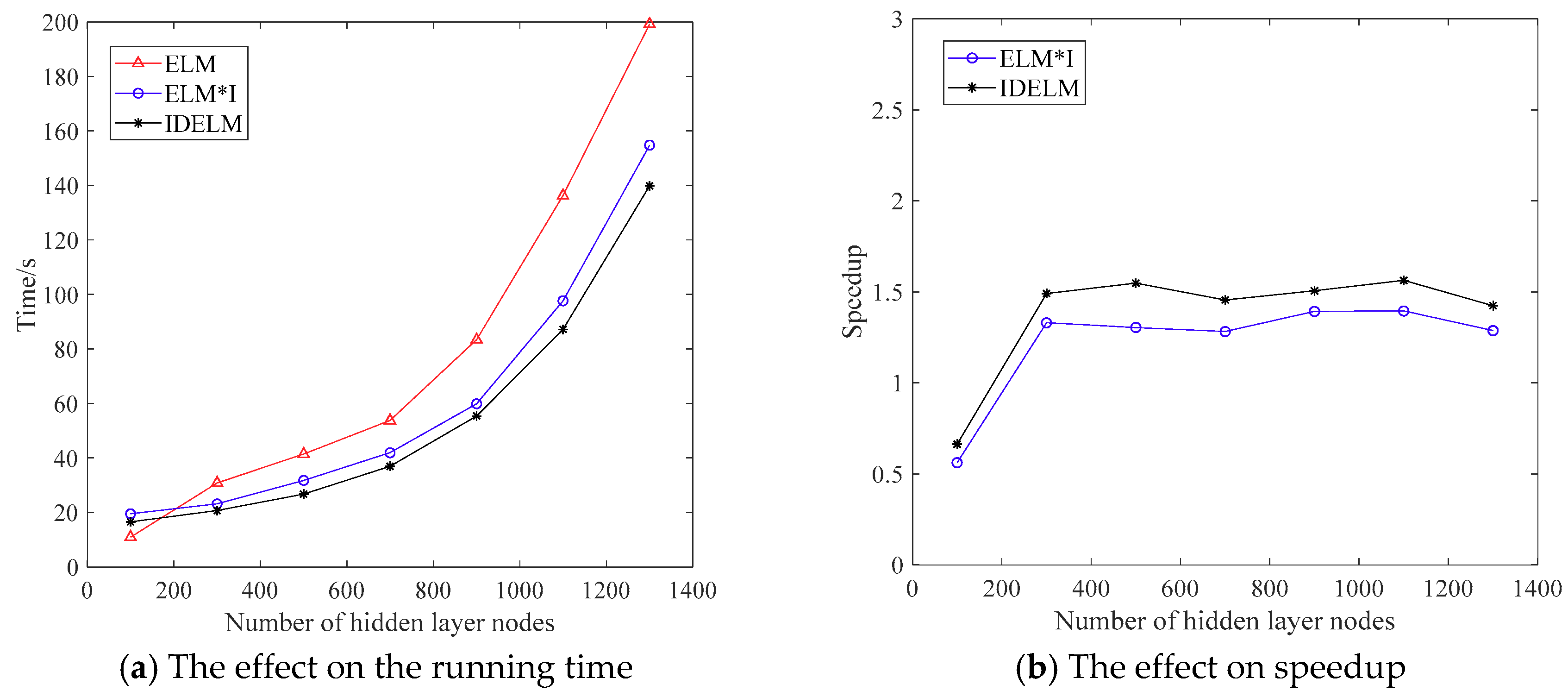
3.3.2. The Effect of Number of Hidden Layer Nodes on the Performance of IDELM Algorithm

In this part, seven sets of experiments are conducted with seven different number of hidden layer nodes. Figure 2 presents the influence of the number of hidden layer nodes on the running time and acceleration ratio of the algorithm. It can be seen from Figure 2a that as the number of hidden layer nodes increases, the running time of the three algorithms all show an upward trend. Among them ELM is the result of stand-alone operation, the other two are the operation result on the distributed cluster. When the hidden layer node is greater than 200, the runtime of single ELM algorithm grows greater than the other two algorithms. The running time of IDELM with the same number of nodes is obvious in the two distributed algorithms less than ELM*I. In theory, distributed ELMs run faster than standalone ELMs, but at the beginning of Figure 2a, the runtime of single ELM is less than the two distributed ELMs, primarily because distributed ELMs require Running on a Hadoop cluster, when a MapReduce program runs on a cluster, a large number of intermediate results are generated inside the cluster, and intermediate results are transmitted and stored in a time-consuming manner. Therefore, when there are fewer hidden nodes, the distributed ELM consumes more time. However, as the number of hidden layer nodes increases, the amount of matrix computation in the algorithm will also increase. As a result of the limitation of stand-alone computing resources and serial ELM algorithm, the growth rate of single ELM operation time will increase. The distributed ELM is executed separately on multiple machines, distributed computing takes less time than that of single ELM, the growth rate is relatively small, Figure 2a coincides with this corollary. The IDELM algorithm is the improvement and optimization of the ELM*I algorithm to transfer and store the result in the middle of the cluster, so it runs faster than ELM*I.

The most obvious change in Figure 2b is that the first point deviates greatly from the other points and the rest of the points keep a straight line. The reason for this is already described in detail in Figure 2a, mainly because of the small amount of data at the beginning, it takes more time to transfer and store the intermediate result of the cluster operation, while the single computer takes less time due to the small amount of data, so the speedup is also smaller. Overall, the speedup of IDELM is greater than the speedup of ELM*I, which shows that IDELM algorithm outperforms the ELM*I algorithm.

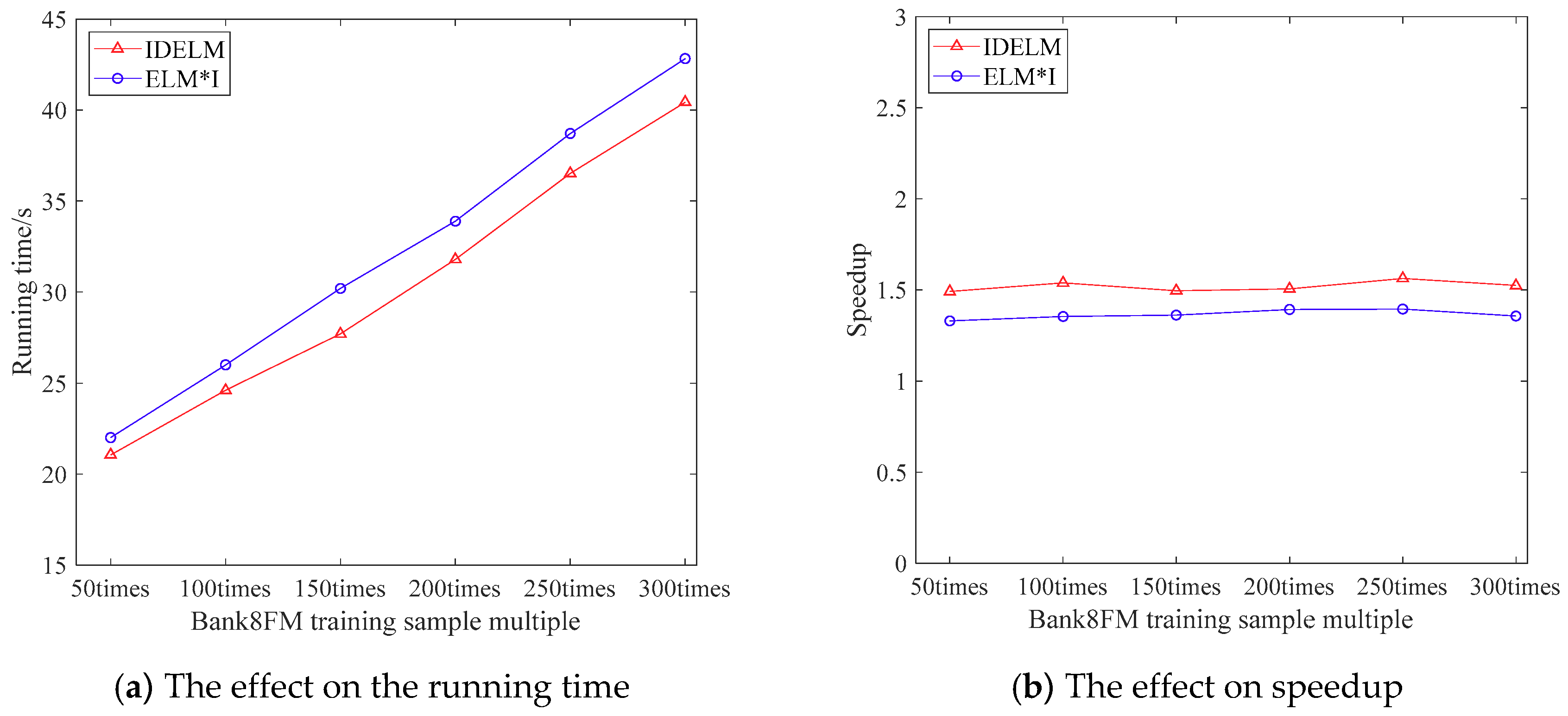
3.3.3. The Effect of Training Sample Number on the Performance of IDELM Algorithm

In order to study the impact of training samples on the running time and speedup of IDELM algorithm, the training samples of Bank8FM data set were artificially extended to 50 times, 100 times, 150 times, 200 times, 250 times and 300 times of the original data set Size of the data set, hidden layer node selected as 10. Figure 3 presents the effect of training samples on the running time and speedup of the algorithm.

It can be seen from Figure 3a that the training time of both algorithms increases linearly with the number of training samples. The running time of the IDELM algorithm is less than the ELM*I algorithm, which shows that the performance of IDELM algorithm is better than ELM*I. At the same time, it can be seen from the Figure 3a that when the number of training samples is increased by tens of times, the increase of training time is very small, which proves that IDELM and ELM*I are suitable for processing high-dimensional data. Figure 3b shows the variation of the acceleration ratios of the two algorithms with the number of training samples. The two lines are almost horizontal and the speedup of IDELM is higher than that of ELM*I.

In summary, both distributed ELM algorithms outperformed the performance of the standalone ELM algorithm, both in terms of the number of hidden layer nodes and the number of training samples. Both experiments prove that the performance of IDELM algorithm is superior to the original ELM*I algorithm, and can effectively deal with the problem of large amounts of high-dimensional data, which has a good application prospect. In practice, with the increase of hidden nodes and the increase of sample data, the performance advantage based on IDELM algorithm will be more obvious.

4. Distributed Particle Swarm Optimization Algorithm

In order to solve the problem of optimizing large-scale data, this paper combines particle swarm optimization with MapReduce algorithm to form a distributed particle swarm optimization (MR-PSO). Figure 4 shows an iterative flow chart of the MR-PSO algorithm. It can be seen from the figure that the whole MR-PSO can be divided into three stages in total: the population initialization stage, the MapReduce stage and the iterative condition determination stage.

4.1. Initialization Stage

When initializing a population, n particles are randomly generated according to a given search space and a uniform distribution function. Then, each particle is put into the fitness function in turn for evaluation. After all the particles are evaluated, the best fitness value of all the particles is selected according to the size of the fitness value and the corresponding particle position is set as the global Best location g_Best. The global optimal particles are then stored in the Distributed File System (DFS) as key-value pair <Key, Value>. The contents of the key-value pair <Key, Value> are stored as shown in Figure 5. The values $i$, $x_i$, $v_i$, $P_{iBest}$, $g_{Best}$, $fitness(x_i)$, $fitness(P_{iBest})$, $fitness(g_{Best})$ are separated by semicolons respectively. They respectively represent the particle $i$, the position of particle $i$, the velocity of particle $i$, The global optimum position, the fitness value of particle $i$, the fitness value of global optimal solution of particle $i$, and the fitness value of global optimal particle.

4.2. MapReduce Stage

In each iteration of PSO algorithm, the MapReduce task needs to be executed. The main task of this MapReduce task is to update the position and velocity of the generation particle swarm based on the previous generation information and then input the next MapReduce task. The pseudo-code that MR-PSO executes in MapReduce is shown in Algorithm 3.

Algorithm 3: MR-PSO algorithm steps

1 class MAPPER

2   method INITIALIZE()

3   position = new ASSOCIATIVEARRAY

4   velocity= new ASSOCIATIVEARRAY

5  method Map( Key:ID,Value:particle)

6    lparticleBest = None;

7    (position,velocity,fitness) = Parse(particle);

9    for each particle do

10      positionNew = position.update(position);

11      velocityNew = velocity.update(velocity);

12      positionNew fitness = Fitness(positionNew);

13      if positionNew fitness> Fitness(lparticleBest)then;

14      lparticleBest =positionNew

15      end if

16      context.write(id,positionNew, velocityNew)

17    end for

18      context.write(localbest, lparticleBest)

19  class REDUCE

20    method reduce(Key : localbest,ValList)

21      gBestparticle = None;

22     for each lparticleBest in ValList do

23      lparticleBest = ParticleLocalBest(VslList)

24      if Fitness(lparticleBest) > Fitness(gBestparticle) then

25       gBestparticle= lparticleBest

26      end if

27     end for

28       context.write(gbestID, gBestparticle);

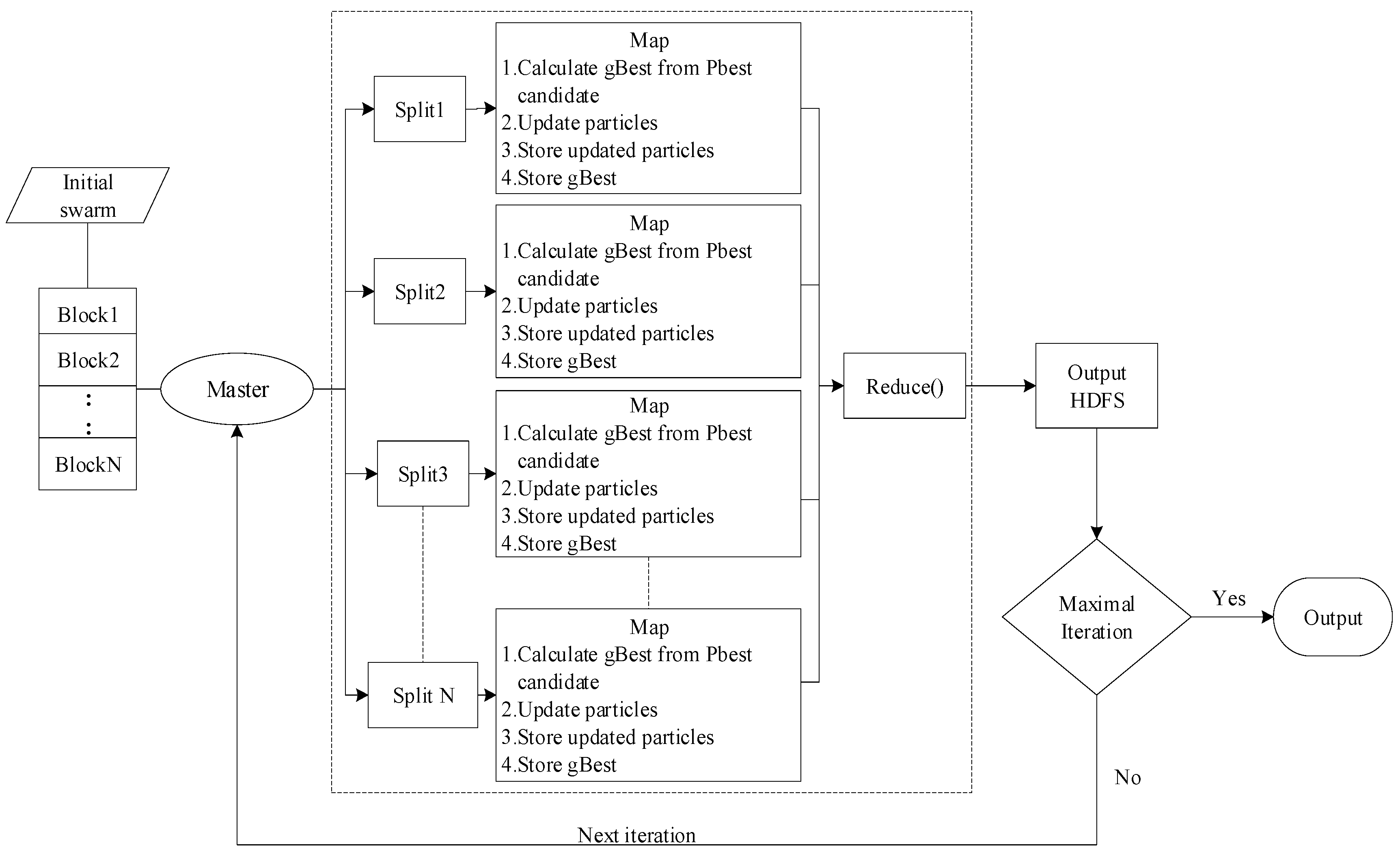
Description of Algorithm 3:

(1)

The input data is divided into a number of data blocks and stored in a distributed file system (HDFS). These data are entered into a MapReduce task as key-value pairs, and then each Map function is assigned a data block;

(2)

The program in Mapper will update the velocity and position of each particle in the data block. After the update, it will bring it into the fitness evaluation function to calculate the fitness value;

(3)

Compare the fitness value of new and old particles, if the fitness value of new particle is good, replace the position of the original particle with the current particle position and store it in HDFS;

(4)

Find the fitness value of the global best particle (lparticle_Best) in each Map, and compare with each updated particle fitness value. If the fitness value of the particle is better than the fitness value of lparticle_Best, use this particle position and velocity replace lparticle_Best position and velocity;

(5)

Through the above particle replacement, the local optimal solution in the current map task is finally obtained, and the local optimal solution is stored into the HDFS in the form of <key, value> key-value pairs, where the key is a fixed value, value is the local optimal particle position;

(6)

When all Map tasks have finished executing, they will be entered into a Reduce task. The main task of Reduce is to find the global best particle ($g_{Best}$) from the lparticle_Best generated from all the Maps, then replace the original global optimal particle and store the final result in HDFS.

4.3. Conditional Judgment Stage

The main task in this stage is to determine whether the number of iterations of MapReduce satisfies the maximum number of iterations or other constraints, and if not, continue to execute the MapReduce task. If the maximum number of iterations is reached, exit the loop and output the global optimum.

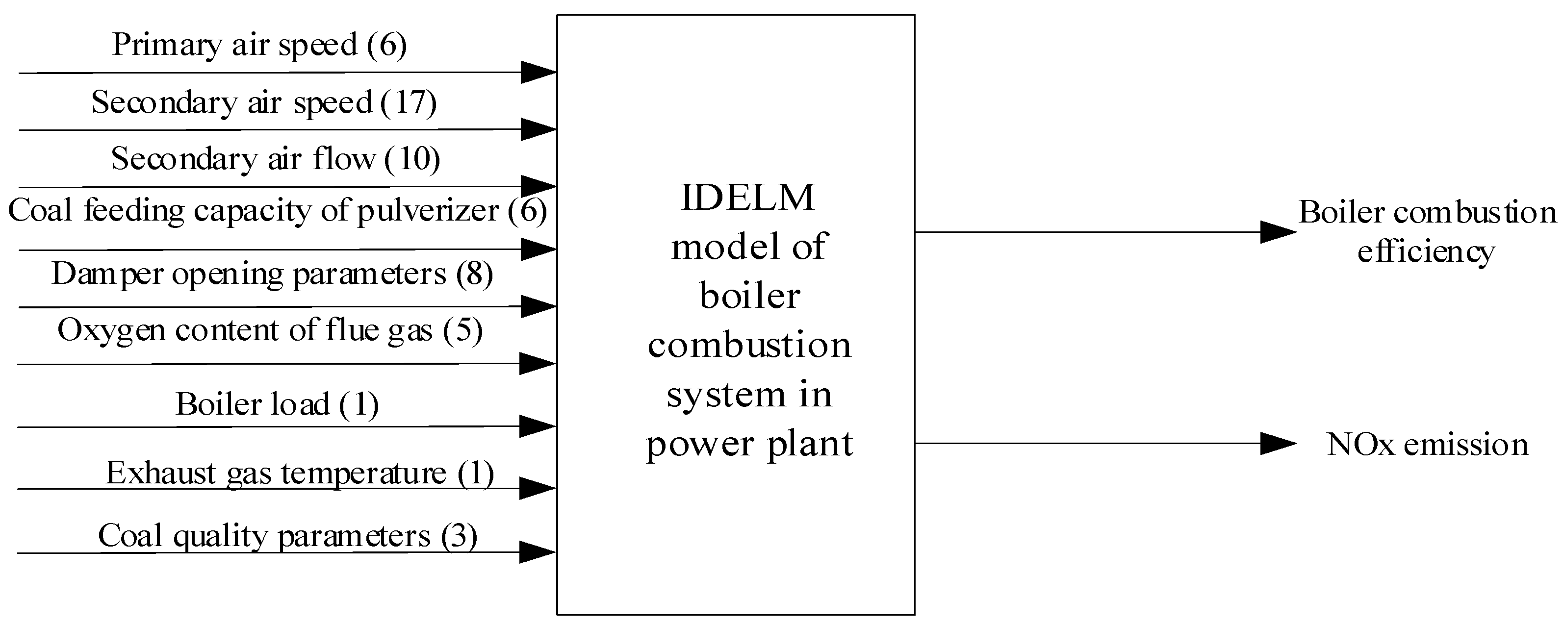
5. Boiler Combustion Model Based on IDELM Algorithm

5.1. Model and Experiments Setup

In this paper, the field operating data of a 660 MW DC solid state slag discharge furnace (pulverized coal-fired boiler) at a power station are used for modeling. Figure 6 shows the boiler combustion model, we can see that the model is affected by a variety of input parameters. For real boiler combustion systems, input parameters that affect the boiler combustion efficiency and NO_x emission can be divided into three categories: adjustable input parameters, non-adjustable input parameters, and measurable but non-adjustable parameters.

Non-adjustable input parameters generally mainly refer to the distribution of the burner, the internal structure, the boiler model and the size of the boiler, etc., if the values of these parameters are to be changed, only the boiler and the burner related equipment can be changed; measurable Non-adjustable parameters are mainly exhaust gas temperature (EGT), coal quality (CQ) data; while the rest of the input parameters are basically adjustable input parameters (Oxygen content of flue gas(OCFG), boiler load (BL), etc.). In Figure 6, the directly adjustable input parameters are primary air speed (PAS), secondary air speed (SAS), secondary air flow (SAF), coal feeding capacity of pulverizer (CFCP), damper opening parameters (DOP). (Section 6.1.2 describes how to optimize these directly adjustable input parameters).

The boiler combustion efficiency data of 25,921 samples in HDFS were normalized, and 18,145 sets of data were selected as the training data of the model. The remaining 7776 sets of data were used as the test samples. As the magnitude and dimension of the experimental data are different, if they are used directly, there may be two negative effects. On the one hand, large numerical variables may overwrite small numerical variables in the modeling process, thus reducing the accuracy of the model. On the other hand, if the dispersion between the data is too large, it may cause the model convergence time is too long or cannot converge, in the training process. In order to ensure the performance of the IDELM model, training samples and test samples need to be normalized before the model training. In this paper, the sample data is normalized to [−1, 1]. The normalized formula is as follows:

$$x^{\ast }=\frac{2\cdot (x-x_{\min })}{x_{\max }-x_{\min }}-1$$

(17)

where x is the original sample before normalization and x* is the normalized sample, x_max and x_min are the maximum and the minimum in the original sample, respectively.

The experimental platform is the same as Section 3.3.1. The configuration of the main node is: 32 Gb memory, an 8-core processor and 1 Tb hard disk, from the node configuration: 16 Gb memory, an 8-core processor and a 1 Tb hard drive. Hadoop version 2.6.2.

5.2. Parameters L and A on IDELM Model

Before the training model, it is necessary to determine the values of the parameter regular term A and the hidden layer node L firstly. These two parameters have a great impact on the performance of the model, and their determination is the best model selection problem.

In this paper, cross-validation method is used to continuously adjust the values of A and L to select the combination with the smallest cross-validation error as the optimal combination of parameters. By calculation, the parameters A and L of the NO_x emission model and the boiler combustion efficiency model are determined as shown in

Table 1. Parameter selection of boiler combustion model.

	Parameter	Value
NOx emission model	Regularization term (A)	28
	Hidden layer node (L)	1010
Boiler combustion efficiency model	Regularization term (A)	26
	Hidden layer node (L)	1000

.

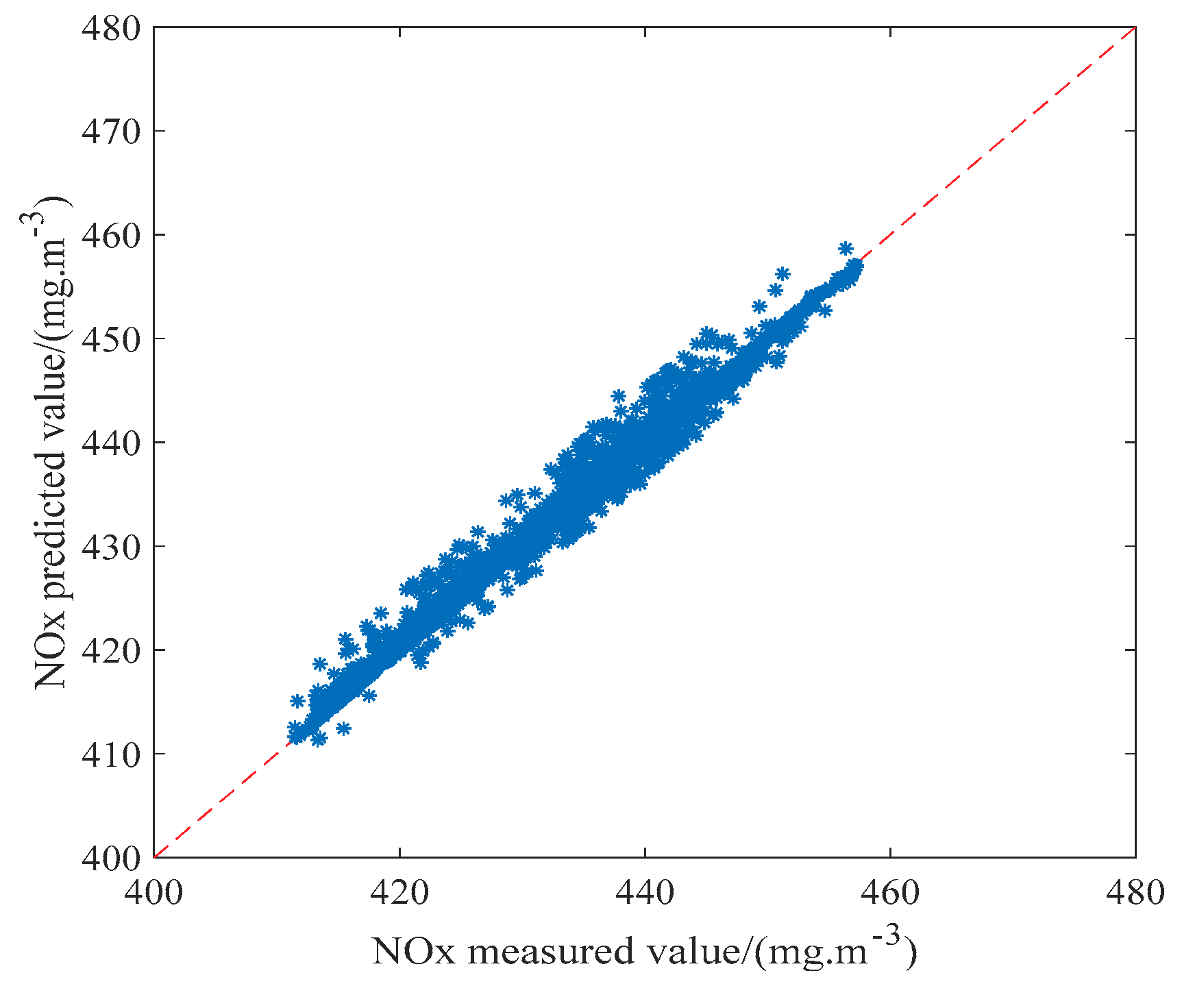
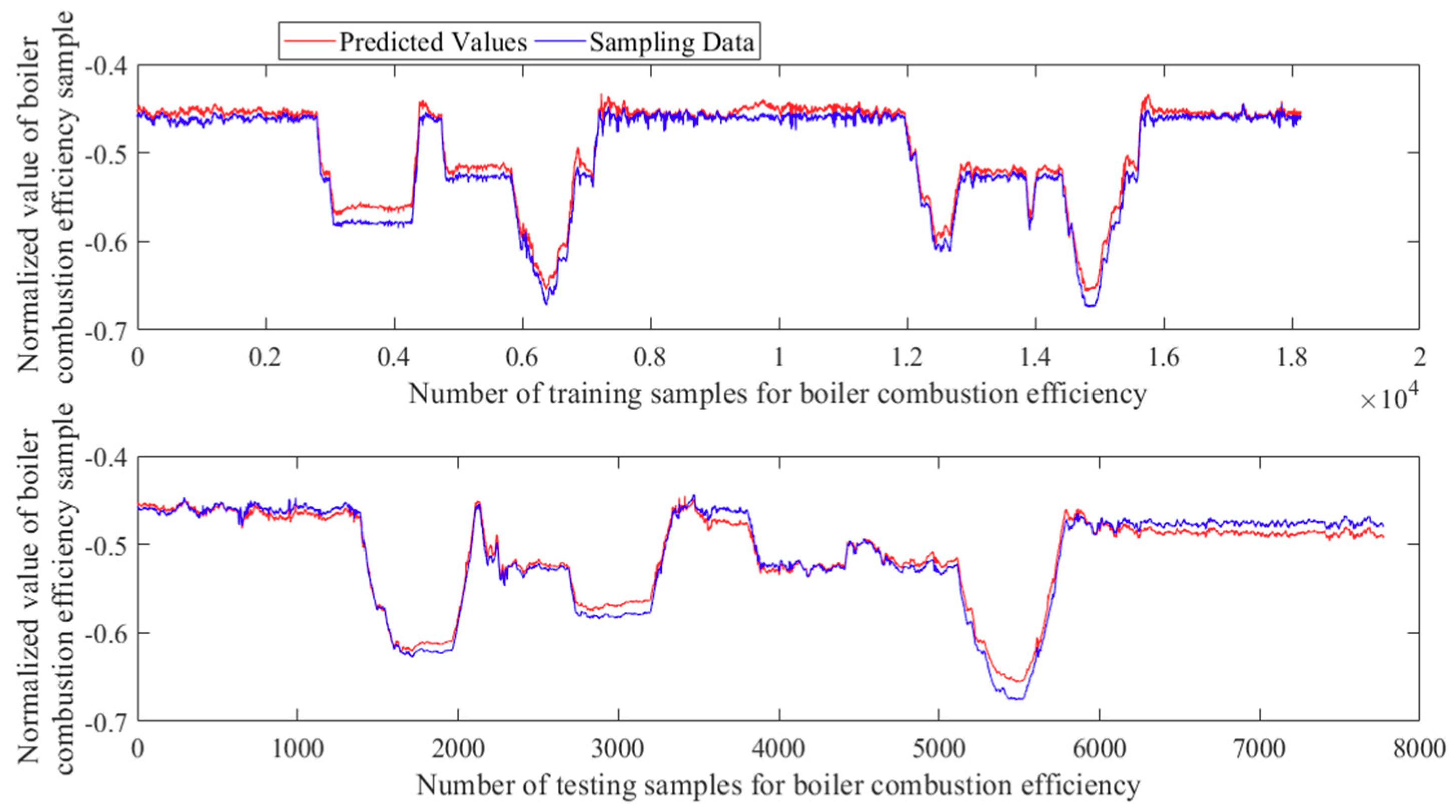
5.3. The Effect of Prediction

In order to verify the predictive ability of the model, root mean squared errors (RMSE), mean relative error (MRE) and coefficient of determination R² are used to evaluate the predictive ability of the model. The specific formula are shown as follows:

$$\mathrm{RMSE}=\sqrt{{\displaystyle \sum _{i=1}^N{(f(x_i)-y_i)}^2/N}}$$

(18)

$$\mathrm{MRE}=\frac{1}{N}{\displaystyle \sum _1^N\left|\frac{f\left(x_i\right)-y_i}{y_i}\right|}$$

(19)

$${\mathrm{R}}^2=1-\frac{{\displaystyle \sum _{i=1}^N(f\left(x_i\right)}-y_i{)}^2}{{\displaystyle \sum _{i=1}^N{(y_i-\overline{y})}^2}}$$

(20)

where $N$ is the number of samples, $f(x_i)$ is the model predictive value, $y_i$ is the corresponding actual measured value, $\overline{y}$ is the average of the actual measurements.

The prediction results of the NO_x test sample on the IDELM model are shown in Figure 7. It can be seen that the predicted value of NO_x and the actual measured values of NO_x are generally distributed around the diagonal, indicating that the IDELM model can predict NO_x emissions very well.

Table 2. Evaluation Index of NO_x emission Model Based on IDELM Algorithm.

NOx	RMSE	MRE	R2
Training set	0.0436	0.0481	0.863
Testing set	0.0313	0.0423	0.891

shows the mean value of 20 test results for RMSE, MRE, and R² for training samples and test samples of NO_x emissions. It can be seen that the error is small, and the error of the test sample is slightly larger than that of the training sample. The determination coefficient R² of the prediction result of the model training sample is 0.863 and the determination coefficient R² of the test sample is 0.891. The result shows that the model has a good ability of fitting and predicting.

Figure 8 is a forecast of the efficiency of the boiler and shows the coincidence between the predicted values of the IDELM model and the sampling data. The ordinate in the graph is negative because the input samples are normalized [−1, 1] before training, the boiler combustion efficiency value is relatively small in the sample data, so the normalized result is negative. It can be seen from the Figure 8 that the predicted values of the training sample or the test sample and the sampling data roughly coincide, indicating that the model has better accuracy and generalization performance.

In order to further verify the predictive ability of the model,

Table 3. Evaluation index of boiler combustion efficiency model based on IDELM algorithm.

Boiler Combustion Efficiency Data	RMSE			MRE			R2
	Max	Min	Means	Max	Min	Means	Max	Min	Means
Training set	0.0189	0.0065	0.0152	0.0361	0.0101	0.0278	0.9876	0.8944	0.9256
Test set	0.0153	0.0087	0.012	0.0227	0.0141	0.0187	0.9766	0.9275	0.9538

shows the test results of the RMSE, MRE, and R² of the training and test samples, their maximum (Max), minimum (Min), and average (Means) values are given. The results of RMSE, MRE, R² in the table are the average of 20 experimental results. Usually RMSE, MRE smaller the more able to respond to the model of high precision, and the R² value closer to 1, indicating that the model better fit. It can be seen from the table that the maximum value of RMSE and MRE in the test sample is smaller than the maximum value of the training sample and the average value is much smaller than that of the training sample, which shows that the model has a great generalization ability. The determination coefficient R² of the test sample is 0.9538, which shows that the model has better fitting and predictive ability.

6. The Realization of Boiler Combustion Optimization

6.1. Optimization Problem Description

6.1.1. Boiler Combustion Optimization Function Design

As boiler combustion optimization involves multi-objective optimization, it is necessary to design an objective function that contains both low NO_x emissions and high boiler combustion efficiency, to combine both technical indicators. However, NO_x emissions and boiler combustion efficiencies have different dimensions. In order to reduce the mutual influence between the two, we need to normalize the two optimization objectives to achieve the same order of magnitude before optimization. In real life, each power station has different requirements on NO_x emissions and boiler combustion efficiency, so the related objective function in the multi-objective function can be weighted. Because the objective of this paper is to find the lowest NO_x emissions and the highest combustion efficiency, this paper uses the subtraction of NO_x emissions and combustion efficiency as the objective function to achieve the goal of the same direction of the optimization. Finally, the two objective functions are combined into a comprehensive objective function according to a certain weight ratio. The combined objective function is as follows:

$$\min f(x)=\alpha \times \frac{f_{NOx}(x)-f_{NOx}(x_{\min })}{f_{NOx}(x_{\max })-f_{NOx}(x_{\min })}-\beta \times \frac{f_{\eta }(x)-f_{\eta }(x_{\min })}{f_{\eta }(x_{\max })-f_{\eta }(x_{\min })}$$

(21)

Let $a=\frac{f_{NOx}(x)-f_{NOx}(x_{\min })}{f_{NOx}(x_{\max })-f_{NOx}(x_{\min })}$, $b=\frac{f_{\eta }(x)-f_{\eta }(x_{\min })}{f_{\eta }(x_{\max })-f_{\eta }(x_{\min })}$, then the above equation can be simplified as:

$$\min f(x)=\alpha \times \mathrm{a}-\beta \times b$$

(22)

where $f_{N{O}_x}(x_{\max })$,$f_{N{O}_x}(x_{\min })$ are the maximum value and minimum value of the actual NO_x emission, $f_{\eta }(x_{\max })$, $f_{\eta }(x_{\min })$ are the maximum value and minimum value of the actual boiler combustion efficiency. $\alpha$, $\beta$ are the weight of each technical indicator, and $\alpha +\beta =1$.

6.1.2. Constraints

In the actual operation of boilers, some parameters cannot be adjusted artificially, such as the layout of boiler equipment, furnace type, structure, and so on, while the operation load, coal quality, exhaust gas temperature and so on cannot be adjusted arbitrarily in practice, although they will change during operation, they cannot be adjusted directly, and they are still regarded as non-adjustable parameters. Adjustable parameters refer to the parameters that the operators can control and adjust in the safe range when the boiler is running.

In Figure 6, the non-adjustable input parameters are oxygen content of flue gas (OCFG, five items), boiler load (BL, one item), exhaust gas temperature (EGT, one item), coal quality parameters (CQ, three items), their values remain unchanged. The adjustable input parameters are relative items of secondary air speed correlation (SAS, SAPB and SAT, 17 items), secondary air flow (SAF, 10 items), coal feeding capacity of pulverizer (CFCP, six items), primary air speed (PAS, six items), Damper opening parameters (DOP, eight items), a total of 47 adjustable input parameters.

Taking the 47 adjustable parameters as optimization parameters, according to the actual data collected by the power plant, the constraints are determined on the premise of ensuring the safe operation of the boiler [28,29], so as to narrow the optimization scope and improve the practicability of the model. The constraints of 47 parameters are shown in Table 4(1)–(4) (notes: SAPB is the secondary air’s pressure bias, SAT is secondary air temperature, the abbreviations for other items are given in Section 5).

6.2. Combustion Optimization Based on MR-PSO Algorithm

In the MR-PSO algorithm, Formula (22) is adopted as the fitness function of distributed particle swarm optimization, that is, the fitness value of each particle is weighted by the values of NO_x emission and boiler combustion efficiency. The flow chart for optimization using the MR-PSO algorithm on the IDELM model is shown in Figure 9.

MR-PSO algorithm to optimize boiler combustion model input parameters of the specific steps are as follows:

(1)

In the experiment, the initialization range of the initial population should be determined according to the actual operating data of the boiler combustion system collected this time, and then randomly generate n particles within the constraint range according to the uniform distribution function and store them into the distributed File system (HDFS);

(2)

The master node shaves input files in HDFS and distributes the sliced data to Map tasks.

(3)

The Map task separates and extracts the particle information from the input file, separates the particle velocity and position information respectively, and updates the particle velocity and position according to the velocity Equation (10) and the position Equation (11), and then substitute the updated particle’s position information into the boiler combustion IDELM model to get the prediction result. The Fitness value is obtained by Equation (22), according to the size of the fitness evaluation value, it is determined whether to replace the original particle velocity and position, and store it in HDFS in a certain order. All the particles are compared with the global optimal particle, replace its value if it is better than the original value, and storing it in the HDFS, thereby obtaining the global optimal particle in the map;

(4)

The main task of Reduce is to compare the local global optimal particles obtained by each map task before, and get the global optimal position of the entire particle swarm, and store it into the HDFS in key-value pairs;

(5)

After the completion of the Reduce task, it is judged whether the maximum number of iterations is satisfied. If the maximum iteration is not satisfied, the Map task is returned to step (3), and the Map task is continued until the maximum number of Iterations is satisfied.

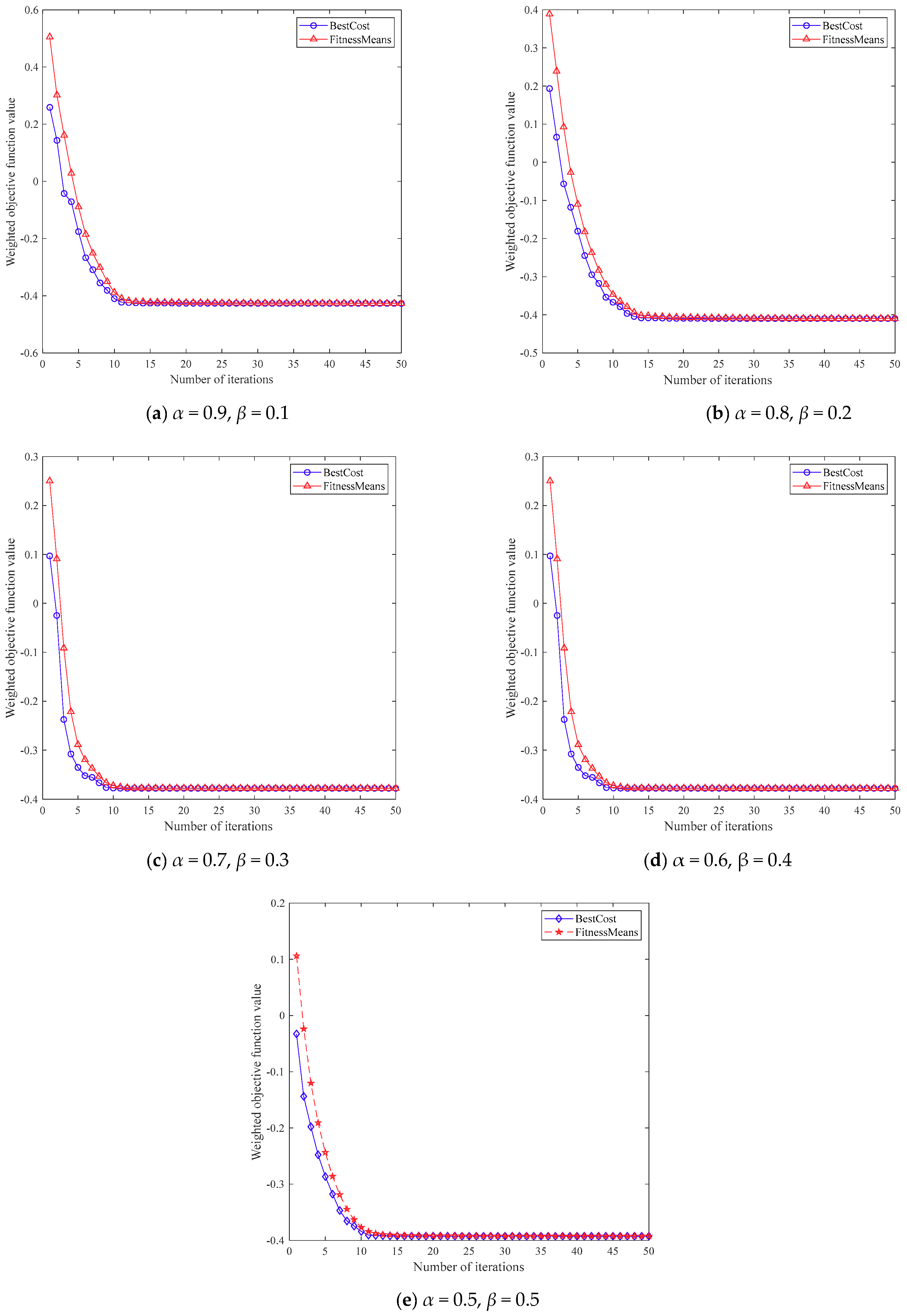
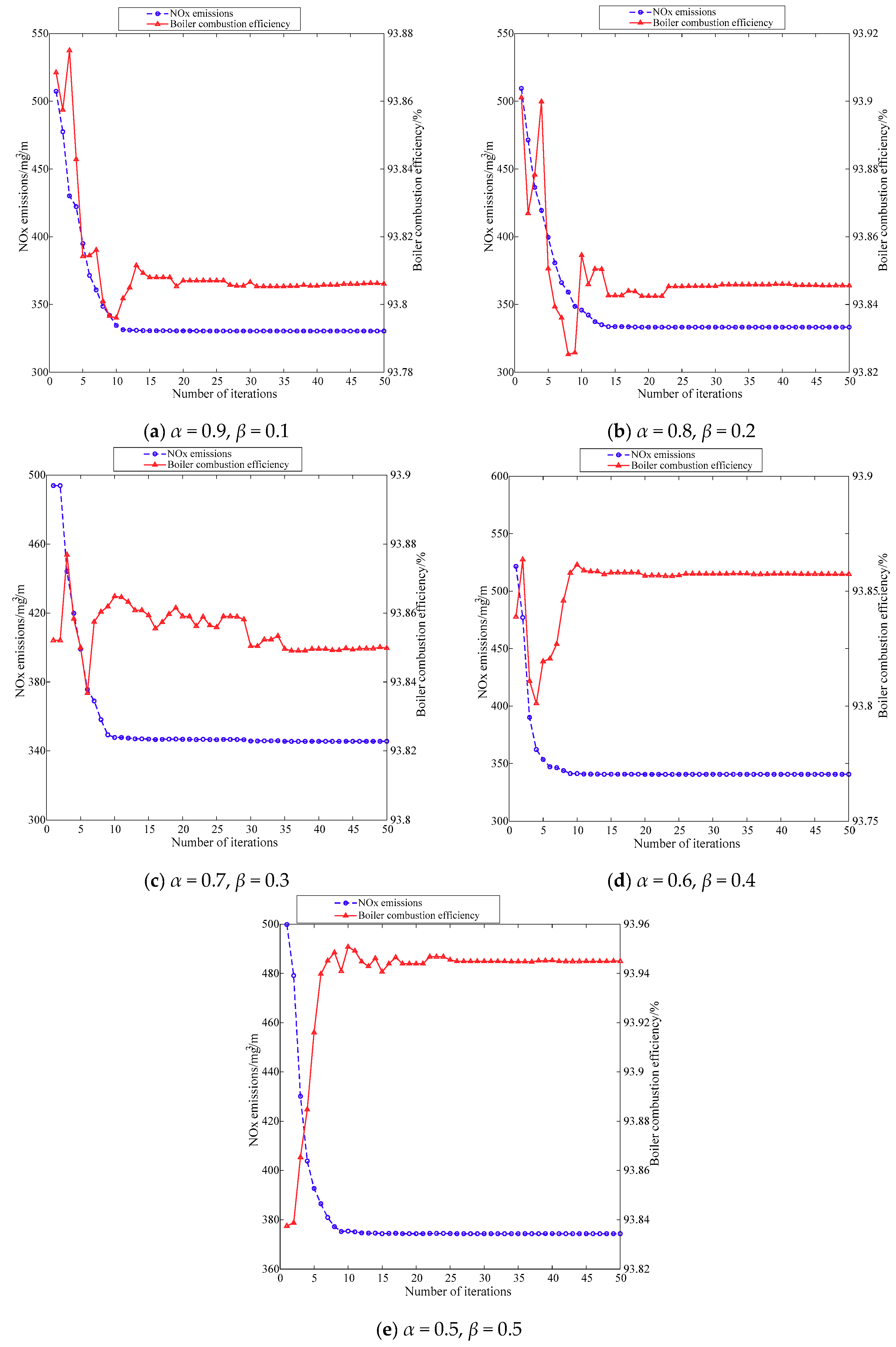
6.3. Analysis of Optimization Results under Different Weights

In this paper, we have optimized the input parameters of the 18,001-th group of conditions with the largest NO_x emissions in the sample data, so as to generate a set of parameters that can reduce the NO_x production and improve the boiler combustion efficiency. The 10 parameter values that are not adjustable in the operating conditions are shown in

Table 5. The value of the non-adjustable parameter.

Working Condition	Boiler Load/MW	Exhaust Temperature/°C	Coal Quality Parameters			Oxygen Content of Flue Gas/%
			Total Moisture/%	Air-Dried Moisture/%	Dry Base Ash/%	Entrance A	Entrance B	Entrance C	Exit A	Exit B
18,001	349.1	129.58	10.6	2.71	31.93	5.35	5.45	5.54	8.37	6.99

. The corresponding NO_x emissions, boiler combustion efficiency and boiler load of the 18,001-th group are 412 mg/m³, 93.39% and 349.1 MW, respectively.

The population number of MR-PSO in the boiler combustion optimization model is 100; the maximum number of iterations is 50; the maximum inertia weight ($w_{\max }$) is 0.9; the minimum inertia weight ($w_{\min }$) is 0.4; and the acceleration factors $c_1$ and $c_2$ are both 2.

The focus of this article is to achieve a reduction in boiler NO_x emissions, so the weight of NO_x is greater than the weight of boiler combustion efficiency. To verify the effect of weight ratio on NO_x emission and boiler combustion efficiency, we choose ($\alpha =0.9,\beta =0.1$), ($\alpha =0.8,\beta =0.2$), ($\alpha =0.7,\beta =0.3$), ($\alpha =0.6,\beta =0.4$), ($\alpha =0.5,\beta =0.5$) to be analyzed.

The MR-PSO algorithm is used to optimize the boiler combustion model under the 18,001th working condition. The curves of the fitness values of the boiler combustion optimization model at different weighting factor ratios are shown in Figure 10a–e. The combustion optimization model under the five weighting ratios ($\alpha =0.9,\beta =0.1$), ($\alpha =0.8,\beta =0.2$), ($\alpha =0.7,\beta =0.3$), ($\alpha =0.6,\beta =0.4$), ($\alpha =0.5,\beta =0.5$) weighted objective function value curve. The optimized output was compared with the original value of condition 18,001.

It can be seen from Figure 10 that the weighted objective function values of the boiler combustion optimization model under different weights gradually decrease with the increase of the number of iterations, except that their respective starting points and decreasing ranges are different. Their convergence speeds are relatively fast, the trend of change in function values around the 15th generation is very small.

Figure 11a–e show the optimized results of NO_x emissions and boiler combustion efficiency at different weighting factor ratios for a boiler combustion optimization model under a load of 349.1 MW.

Observing Figure 11a, the NO_x emissions and boiler combustion efficiency decrease sharply at the beginning and stabilize after 20 cycles, resulting in NO_x emissions of 330.42 mg/m³ and boiler combustion efficiency of 93.81%. Comparing with the 412 mg/m³ of NO_x emissions and 93.39% of boiler combustion efficiency under the initial conditions, after optimization, the NO_x emissions are reduced by 19.8% and the boiler combustion efficiency is improved by 0.45%, which is in line with the purpose of reducing NO_x emission and improving boiler combustion efficiency.

Observing Figure 11b, the NO_x emissions and boiler combustion efficiency also decrease sharply at the beginning and stabilize after about 25 generations. The optimized NO_x emissions result is 333.29 mg/m³ and the boiler combustion efficiency is 93.84%. Comparing with Figure 11a, the NO_x emissions and boiler combustion efficiency all increase, but the increase is not significant. Comparing with the data under the original conditions, the optimized NO_x emissions are reduced by 19.1%, and the optimized boiler combustion efficiency is improved by 0.48%.

Observing Figure 11c, the rate of decline in NO_x emissions and boiler combustion efficiency in Figure 11c is significantly less than in Figure 11a,b. Boiler combustion efficiency has been in the range of [93.84%, 93.87%], and stabilizes around 35 generations later. Finally, the NO_x emissions optimization result is 345.56 mg/m³ and the boiler combustion efficiency is 93.85%. Compared to the pre-optimization data, the optimized NO_x emissions are reduced by 19.1% and the optimized boiler combustion efficiency is reduced by 0.49%.

The most noticeable change observed in Figure 11d is that the boiler combustion efficiency drops sharply in previous generations and then slowly increases. Comparing with Figure 11a, and Figure 11b,c, the general trend of boiler combustion efficiency is rising in Figure 11d. This may be due to the increase of boiler combustion efficiency weight ratio. The final NO_x emissions result was 340.6 mg/m³ and the boiler combustion efficiency was 93.86%. The optimized NO_x emissions were reduced by 17.3% and the boiler combustion efficiency by 0.5% compared to the pre-optimization data.

Comparing with the first four pictures, it can be clearly seen that the boiler combustion efficiency in Figure 11e shows an upward trend, and the fluctuation amplitude after the 10-th generation is also significantly smaller than that of the first four pictures and finally reaches 93.945%. Moreover, the rate of NO_x emissions decline is also significantly less than the previous figures, and the final optimization result is 374.35 mg/m³. This is because the weight ratio of NO_x emissions to boiler combustion efficiency is 5:5, and the NO_x reduction is no longer emphasized. Comparing to the pre-optimization data, the optimized NO_x emissions are reduced by 9.14% and the boiler combustion efficiency is reduced by 0.6%.

The optimization results of the tunable parameters after adjusting the boiler combustion optimization models with different weight ratios under the condition 18,001 are shown in Table 6(1)–(6) (notes: Pre represents pre-optimization, Post represents post-optimization).

Through the comparison between pre-optimization and post-optimization in the table, we can see that the NO_x emission decrease after optimization, and the NO_x emission increases slowly with the decrease of the weight. Boiler combustion efficiency increases after optimization and increases as the weight increases.

From the table of the overall data, it can be seen that, primary air volume increases after optimization, so that of pulverized coal combustion can be fully; after optimization, the secondary air speed and secondary air flow decline, and its reduction is conducive to reducing NO_x generated. The decrease of secondary air flow indicates that the furnace oxygen decreases, the decrease of furnace oxygen can reduce the thermal NO_x and fuel NO_x formation, thereby reducing the formation of NO_x. With the damper opening to variation degrees, it is conducive to burn out of incomplete combustion products, then it can reduce NO_x emissions and prevent furnace coking. The burn-in damper is closed before optimization, which is why the pre-optimization NO_x emissions are very high and the boiler combustion efficiency is relatively low. The amount of pulverized coal from coal mill maintains the overall unchanged.

7. Conclusions

With the deepening of power plant intellectualization, the trend towards large amounts of high-dimensional power plant system data is inevitable. In this paper, the field operation data of a 660 MW power plant combustion boiler (a pulverized coal-fired boiler) are used for modeling and optimization. Because of the large amount of data, the single machine runs slowly and cannot be processed, so Extreme Learning Machine (ELM) parallelization is realized by using the MapReduce framework of Hadoop, a popular data platform in recent years. An improved Distributed Extreme Learning Machine (IDELM) is proposed and applied to boiler combustion system modeling.

Due to the need to consider both low NO_x emissions and high boiler combustion efficiency, this involves multi-objective optimization. The multi-objective function of the boiler combustion system is established by a weight coefficient method, and the multi-objective optimization model of boiler combustion is established by an IDELM algorithm, in order to reduce the emissions of NO_x and improve the boiler combustion efficiency of boiler as much as possible. The distributed transformation of particle swarm optimization (PSO) algorithm based on a MapReduce framework is carried out, and the adjustable input parameters of the boiler combustion model are optimized by MR-PSO, finally obtaining the optimal combination of a set of adjustable input parameters, to achieve low NO_x emissions and high boiler combustion efficiency. The results of this implementation reveal a good performance of the proposed method for optimization of power plant boiler combustion.

References

1. BeloševićaIvan, S.; Tomanović, I.; Beljanski, V.; Tucaković, D.; Živanović, T. Numerical prediction of processes for clean and efficient combustion of pulverized coal in power plants. Appl. Therm. Eng. 2015, 74, 102–110. [Google Scholar] [CrossRef]
2. Barnes, D.I. Understanding pulverised coal, biomass and waste combustion—A brief overview. Appl. Therm. Eng. 2015, 74, 89–95. [Google Scholar] [CrossRef]
3. Zhou, H.; Zhao, J.P.; Zheng, L.G.; Wang, C.L.; Cen, K.F. Modeling NOx emissions from coal-fired utility boilers using support vector regression with ant colony optimization. Eng. Appl. Artif. Intell. 2012, 25, 147–158. [Google Scholar] [CrossRef]
4. Wu, X.Y.; Tang, Z.H.; Cao, S.X. A hybrid least square support vector machine for boiler efficiency prediction. In Proceedings of the 2017 IEEE 3rd Information Technology and Mechatronics Engineering Conference (ITOEC), Chongqing, China, 3–5 October 2017. [Google Scholar] [CrossRef]
5. Lu, Y.K.; Peng, X.; Zhao, K. Hybrid Modeling Optimization of Thermal Efficiency and NOx Emission of Utility Boiler. J. Chin. Soc. Electr. Eng. 2011, 31, 16–22. [Google Scholar] [CrossRef]
6. Huang, G.B.; Zhu, Q.Y.; Siew, C.K. Extreme learning machine: A new learning scheme of feedforward neural networks. Neural Netw. 2004, 2, 985–990. [Google Scholar] [CrossRef]
7. Huang, G.B.; Zhu, Q.Y.; Siew, C.K. Extreme learning machine: Theory and applications. Neurocomputing 2006, 70, 489–501. [Google Scholar] [CrossRef] [Green Version]
8. Liu, H.; Li, F.; Xu, X.; Sun, F. Multi-modal local receptive field extreme learning machine for object recognition. Neurocomputing 2018, 277, 4–11. [Google Scholar] [CrossRef]
9. Huang, G.B.; Zhou, H.; Ding, X.; Zhang, R. Extreme learning machine for regression and multiclass classification. IEEE Trans. Syst. Man Cybern. Part B 2012, 42, 513–529. [Google Scholar] [CrossRef] [PubMed]
10. Huang, G.B.; Chen, L. Enhanced random search based incremental extreme learning machine. Neurocomputing 2008, 71, 3460–3468. [Google Scholar] [CrossRef] [Green Version]
11. Feng, G.; Huang, G.B.; Lin, Q.; Gay, R. Error minimized extreme learning machine with growth of hidden nodes and incremental learning. IEEE Trans. Neural Netw. 2009, 20, 1352–1357. [Google Scholar] [CrossRef]
12. Zhao, X.; Wang, G.; Bi, X.; Zhao, Y. XML document classification based on ELM. Neurocomputing 2011, 74, 2444–2451. [Google Scholar] [CrossRef]
13. Zong, W.; Huang, G.B. Face recognition based on extreme learning machine. Neurocomputing 2011, 74, 2541–2551. [Google Scholar] [CrossRef]
14. Mohammed, A.A.; Minhas, R.; Wu, Q.M.J.; Sid-Ahmed, M.A. Human face recognition based on multidimensional PCA and extreme learning machine. Pattern Recognit. 2011, 44, 2588–2597. [Google Scholar] [CrossRef]
15. Tan, P.; Xia, J.; Zhang, C.; Fang, Q.Y.; Chen, G. Modeling and reduction of NOx emissions for a 700 MW coal-fired boiler with the advanced machine learning method. Energy 2016, 94, 672–679. [Google Scholar] [CrossRef]
16. Li, G.; Niu, P.; Ma, Y.; Wang, H.; Zhang, W. Tuning extreme learning machine by an improved artificial bee colony to model and optimize the boiler efficiency. Knowl. Based Syst. 2014, 67, 278–289. [Google Scholar] [CrossRef]
17. Wu, B.; Yan, T.H.; Xu, X.S.; He, B.; Li, W.H. A MapReduce-Based ELM for Regression in Big Data. In Proceedings of the International Conference on Intelligent Data Engineering and Automated Learning, Yangzhou, China, 12–14 October 2016; Springer: Cham, Switzerland, 2016; pp. 164–173. [Google Scholar] [CrossRef]
18. Luo, M.; Zhang, L.; Liu, J.; Guo, J.; Zheng, Q. Distributed extreme learning machine with alternating direction method of multiplier. Neurocomputing 2017, 261, 164–170. [Google Scholar] [CrossRef]
19. Xin, J.; Wang, Z.; Chen, C.; Ding, L.; Wang, G.; Zhao, Y. ELM*: Distributed extreme learning machine with MapReduce. World Wide Web 2014, 17, 1189–1204. [Google Scholar] [CrossRef]
20. Dean, J.; Ghemawat, S. MapReduce: A flexible data processing tool. Commun. ACM 2010, 53, 72–77. [Google Scholar] [CrossRef]
21. Dean, J.; Ghemawat, S. MapReduce: Simplified data processing on large clusters. Commun. ACM 2008, 51, 107–113. [Google Scholar] [CrossRef]
22. McKenna, A.; Hanna, M.; Sivachenko, E.B.A.; Sivachenko, A.; Cibulskis, K.; Kernytsky, A.; Garimella, K.; Altshuler, D.; Gabriel1, S.; Daly, M.; et al. The Genome Analysis Toolkit: A MapReduce framework for analyzing next-generation DNA sequencing data. Genome Res. 2010, 20, 1297–1303. [Google Scholar] [CrossRef]
23. Ramírez-Gallego, S.; Fernández, A.; García, S.; Chen, M.; Herreraa, F. Big data: Tutorial and guidelines on information and process fusion for analytics algorithms with MapReduce. Inf. Fusion 2018, 42, 51–61. [Google Scholar] [CrossRef]
24. Afrati, F.; Stasinoppulos, N.; Ullman, J.D.; Vassilakopoulos, A. Sharesskew: An algorithm to handle skew for joins in mapreduce. Inf. Syst. 2018, 77, 129–150. [Google Scholar] [CrossRef]
25. Shvachko, K.; Kuang, H.; Radia, S.; Chansler, R. The hadoop distributed file system. Mass storage systems and technologies (MSST). In Proceedings of the 2010 IEEE 26th Symposium on Mass Storage Systems and Technologies (MSST), Incline Village, NV, USA, 3–7 May 2010. [Google Scholar] [CrossRef]
26. Eberhart, R.; Kennedy, J. A new optimizer using particle swarm theory. In Proceedings of the Sixth International Symposium on Micro Machine and Human Science, Nagoya, Japan, 4–6 October 1995. [Google Scholar] [CrossRef]
27. Shi, Y.; Eberhart, R. A modified particle swarm optimizer. Evolutionary Computation Proceedings, 1998. In Proceedings of the 1998 IEEE International Conference on Evolutionary Computation Proceedings. IEEE World Congress on Computational Intelligence (Cat. No.98TH8360), Anchorage, AK, USA, 4–9 May 1998. [Google Scholar] [CrossRef]
28. Duda, P.; Dwornicka, R. Optimization of heating and cooling operations of steam gate valve. Struct. Multidiscip. Optim. 2010, 40, 529. [Google Scholar] [CrossRef]
29. Duda, P.; Rząsa, D. Numerical method for determining the allowable medium temperature during the heating operation of a thick-walled boiler element in a supercritical steam power plant. Int. J. Energy Res. 2012, 36, 703–709. [Google Scholar] [CrossRef]
Figure 1. MapReduce working principle.
Energies 12 01036 g001
Figure 2. The effect of the number of hidden layer nodes on the running time (a) and speedup of the algorithm (b).
Energies 12 01036 g002
Figure 3. The effect of training samples on the running time (a) and speedup (b) of the algorithm.
Energies 12 01036 g003
Figure 4. Iterative flow chart of the MR-PSO algorithm.
Energies 12 01036 g004
Figure 5. The structure of particles stored in DFS.
Energies 12 01036 g005
Figure 6. IDELM model of boiler combustion system.
Energies 12 01036 g006
Figure 7. NOx comparison between predicted and measured values.
Energies 12 01036 g007
Figure 8. Prediction of boiler combustion efficiency.
Energies 12 01036 g008
Figure 9. Boiler combustion optimization by MR-PSO Algorithm.
Energies 12 01036 g009
Figure 10. The change curve of the weighted objective function value corresponding to the weight ratio.
Energies 12 01036 g010
Figure 11. Optimization results of NOx emissions and boiler combustion efficiency under different weight ratio.
Energies 12 01036 g011