Multistage Expansion Co-Planning of Integrated Natural Gas and Electricity Distribution Systems

Abstract

This paper focuses on expansion co-planning studies of natural gas and electricity distribution systems. The aim is to develop a mixed-integer linear programming (MILP) model for such problems to guarantee the finite convergence to optimality. To this end, at first the interconnection of electricity and natural gas networks at demand nodes is modelled by the concept of energy hub (EH). Then, mathematical model of expansion studies associated with the natural gas, electricity and EHs are extracted. The optimization models of these three expansion studies incorporate investment and operation costs. Based on these separate planning problems, which are all in the form of mixed-integer nonlinear programming (MINLP), joint expansion model of multi-carrier energy distribution system is attained and linearized to form a MILP optimization formulation. The presented optimization framework is illustratively applied to an energy distribution network and the results are discussed.

1. Introduction

In the era of modern energy systems, electricity and natural gas networks are becoming more and more interdependent [1,2,3,4]. It is therefore essential to run integrated studies of electricity and gas systems to improve the overall efficiency of the energy system. Consequently, planning and operation studies of integrated gas and electricity systems have been of great interest in new publications [1,2,3,4,5,6,7,8,9,10,11,12,13,14,15,16]. In Reference [2], an optimization model is proposed for multi-time period combined gas and electricity networks aimed at minimizing costs associated with gas supply, storage and line pack management as well as electricity generation and load shedding. Stochastic models based on the Monte Carlo simulation are developed in Reference [3,4] to perform day-ahead scheduling and obtain energy flow solution for integrated natural gas and electricity power systems, respectively. In Reference [5], a two-stage stochastic look-ahead dispatch is proposed for integrated electricity power and gas systems which can adjust the improper day-ahead dispatch plan (Stage 1) in the second stage. A datamining technique called decision tree (DT) is utilized in Reference [6] to develop a systemic security dispatch method for integrated natural gas and power systems. In Reference [7], a multi-area, multi-stage model is proposed to integrate the long-term expansion planning studies of generation and transmission of natural gas and electricity systems. An optimization model is developed in Reference [8] to reach optimal expansion plans for gas power plants, electricity transmission lines and gas pipelines in terms of social welfare. In order to study the coordinated operation of natural gas and electricity systems in the presence of power system uncertainties, a robust co-optimization scheduling model is proposed in Reference [9]. Optimal energy flow problem is considered in Reference [10], where some effective models are proposed to identify the solvability of optimal energy flow problem. In Reference [11], a probabilistic reliability-based model is proposed to determine the optimal electricity transmission grid and natural gas network topologies to interconnect various energy hubs. Long-term expansion planning of energy hubs with multiple energy carriers taking into account the energy efficiency, reliability and emission considerations is performed in Reference [12]. In Reference [13], a novel expansion co-planning framework is developed in a combined energy market which takes into account the market uncertainty and demand response impacts.

However, although a wide range of studies on gas and electricity systems integration at bulk generation and transmission levels are available in the literature, a few works have been dedicated to planning and operation studies of such integrated energy systems at distribution level. Nonetheless, high penetration of natural gas-based distributed generation (DG) units in distribution networks calls for more interdependent gas and electricity distribution systems (especially in fast-growing economies) [14]. A detailed discussion on the importance of collaborative gas and electricity distribution systems studies in real-life problems can be found in Reference [14], where a mixed-integer nonlinear programming (MINLP) model is derived for co-expansion planning studies of integrated distribution networks. However, gas consumption of DG units is considered as the only interaction between the electricity and natural gas networks. In other words, heat production of combined heat and power (CHP) units which can reduce gas demand, is not taken into account in Reference [14]. In Reference [15], a chance constrained programming model is proposed for integrated planning of natural gas and electricity distribution networks which minimizes investment and operating cost of gas-fired DGs as well as construction cost of gas pipelines. However, electricity distribution network expansion is not considered. A nonlinear framework is proposed in Reference [16] for optimal placing and sizing of natural gas fired DG units within a multicarrier energy distribution network considering operating costs, network loss and network reliability criteria. In this framework, the heat production of CHP units are also included. Nevertheless, expansion of natural-gas distribution network is eliminated in this reference, although high penetration of gas-fired units can place a costly burden on this system. More importantly, most of the models presented in such studies are mixed-integer nonlinear programming (MINLP) for which convergence to global optimum solution cannot be guaranteed.

Motivated by the aforementioned points, this paper aims to propose a mixed-integer linear programming (MILP) model for natural gas and electricity distribution networks co-planning studies considering different energy hubs (EH). The proposed model takes into account optimal expansion of both electricity and natural gas networks as well as sizing, placement and operation of DG units. In this study, the concept of EH is employed to systematically model the interaction between gas and electricity networks at demand nodes. Extracting the mathematical model of co-planning problem, it is discussed that this model forms a MINLP optimization problem. Hence, in order to guarantee the finite convergence to optimality, the MILP model of co-expansion planning is extracted from linearization of the aforementioned MINLP problem. The proposed model is then applied to a test energy distribution network and the obtained results are discussed in detail. Accordingly, the main contributions of this paper are as follows:

• Developing a MILP model for co-expansion planning of EHs, natural gas and electricity distribution grids
• Modelling the impacts of autonomous DG units on natural gas and electricity distribution networks using the EH concept
• Deriving a novel mixed-integer linear formulation for natural gas distribution system expansion planning
• Taking into account the effect of recovered heat from gas-fired DG units on heat demand reduction.

2. Methodology

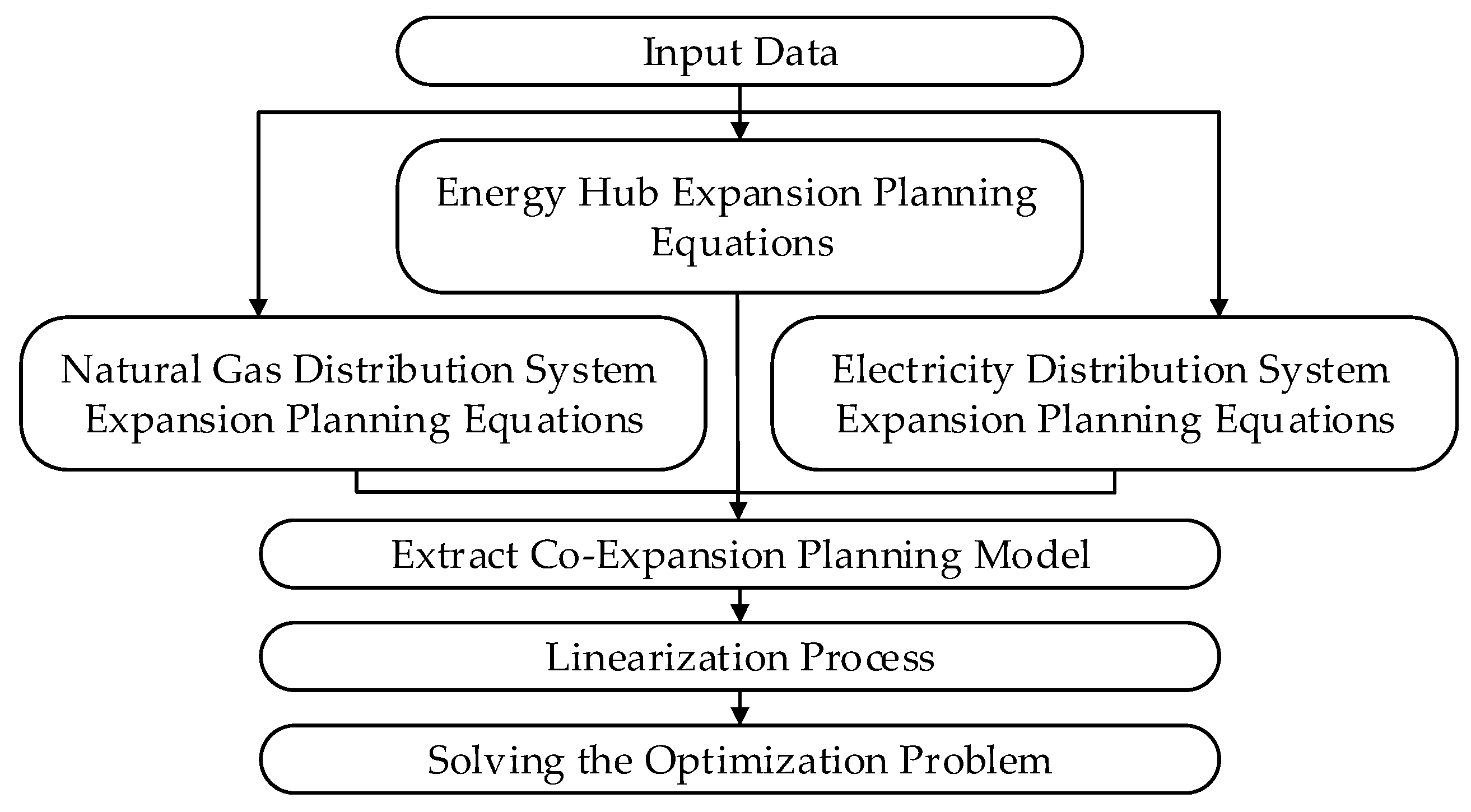
2.1. General Structure of the Proposed Framework

The general structure of the proposed framework is illustrated in Figure 1. According to this figure, the problem modelling starts with the formulation of three general parts of multi-carrier energy distribution systems, that is, energy hub, natural gas distribution system and electricity distribution network expansion planning problems. Subsequently, the co-expansion planning model is extracted from the combination of these three sets of equations. As will be shown, this model is a MINLP optimization problem for which obtaining a global optimal solution could not be guaranteed. Hence, in the next step, some accurate linear approximations are employed to handle nonlinearities and derive a MILP model. Finally, this MILP problem can be solved by standard mathematical programming optimization algorithms to acquire the global optimal expansion plan.

2.2. Problem Formulation

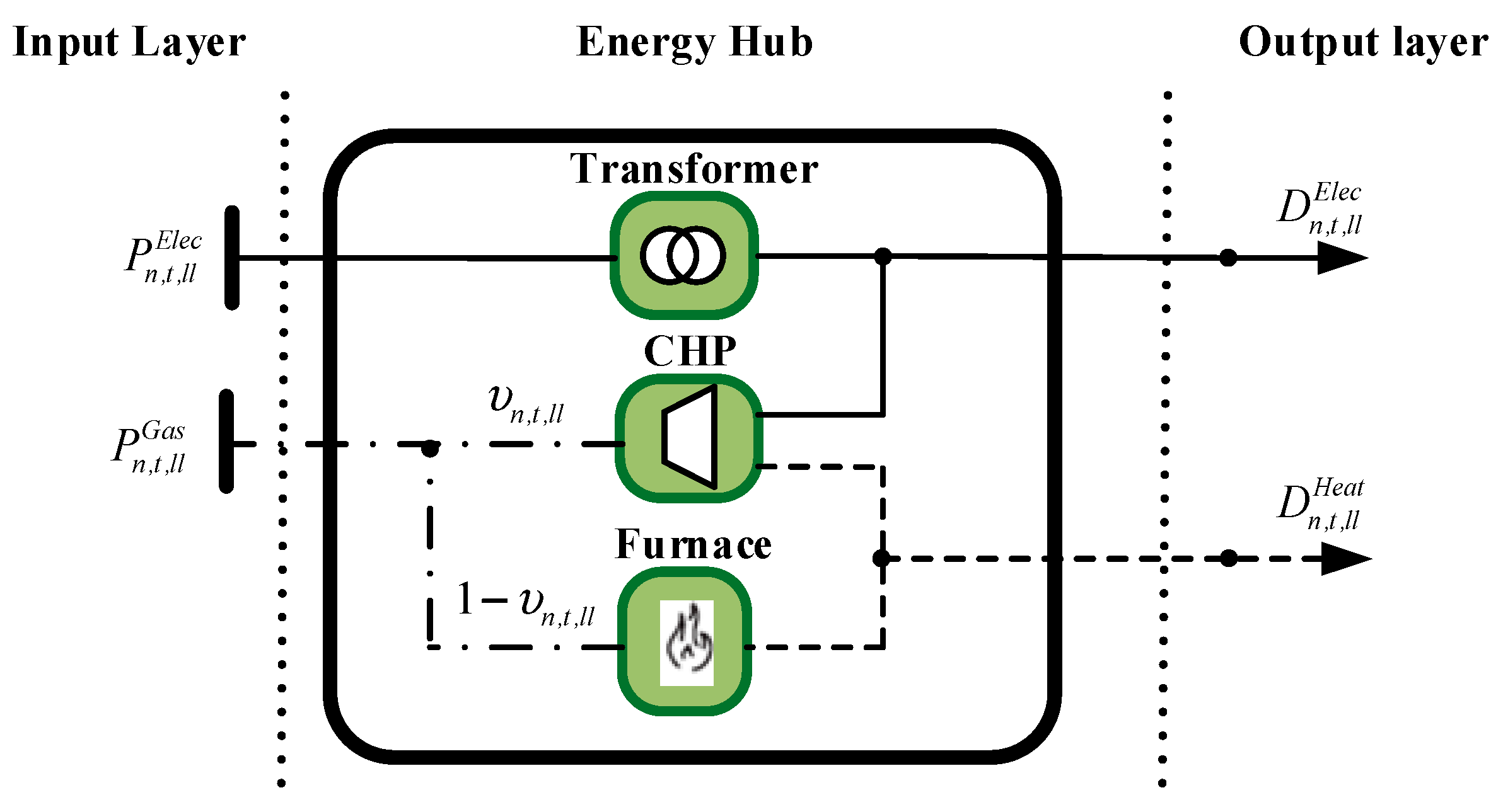
2.2.1. Expansion Planning of Energy Hubs

As stated previously, in this paper, demand of energy carriers in different nodes of electricity and natural gas distribution networks are modelled via energy hubs. This allows for accurate modelling of the interaction between natural gas and electricity infrastructures at the load points [17,18]. General structure of the proposed energy hub is depicted in Figure 2.

Input energy carriers of the energy hub are considered as grid electricity and the natural gas. Received natural gas from the network is dispatched between CHP unit and furnace based on a dispatch factor (${\upsilon }_{n,t,ll}$) [19]. Then, the CHP unit would supply a portion of electricity and heat demand [19].

In EH planning, the objective is to find optimal size of EH components, that is, transformer, CHP unit and furnace to efficiently meet the electricity and heat demand at the output layer. In this respect, the EH cost function which is comprised of the present value of the total investment and operating costs of EHs is given by Equation (1.a), where, N_h and N_L are number of EHs and load levels, respectively.

$${\mathrm{CF}}^{EH}={\displaystyle {\sum }_{t\in T}\left({\delta }_{t,Inv}In{v}_t^{EH}+{\delta }_{t,Op}O{p}_t^{EH}\right)}$$

(1.a)

$$In{v}_t^{EH}={\displaystyle {\sum }_{n=1}^{N_h}(I{C}^{CHP}NC{a}_{n,t}^{CHP}+I{C}^{Fur}NC{a}_{n,t}^{Fur}+I{C}^{Tra}NC{a}_{n,t}^{Tra})}$$

(1.b)

$$\begin{array}{ll}O{p}_t^{EH}=& {\displaystyle {\sum }_{n=1}^{N_h}{\displaystyle {\sum }_{ll=1}^{N_L}D{u}_{t,ll}(P_{n,t,ll}^{Elec}P{r}_{t,ll}^{Elec}+P_{n,t,ll}^{Gas}P{r}_{t,ll}^{Gas}}}+{\eta }^{Tra}{P}_{n,t,ll}^{Elec}O{C}^{Tra}\\ & +{\eta }_{ge}^{CHP}{\upsilon }_{n,t,ll}{P}_{n,t,ll}^{Gas}O{C}^{CHP}+{\eta }^{Fur}(1-{\upsilon }_{n,t,ll})P_{n,t,ll}^{Gas}O{C}^{Fur})\end{array}$$

(1.c)

$${\eta }^{Tra}{P}_{n,t,ll}^{Elec}+{\eta }_{ge}^{CHP}{\upsilon }_{n,t,ll}{P}_{n,t,ll}^{Gas}=D_{n,t,ll}^{Elec}\hspace{0.17em}$$

(2)

$${\eta }^{Fur}(1-{\upsilon }_{n,t,ll})P_{n,t,ll}^{Gas}+{\eta }_{gh}^{CHP}{\upsilon }_{n,t,ll}{P}_{n,t,ll}^{Gas}=D_{n,t,ll}^{Heat}$$

(3)

$${\eta }_{ge}^{CHP}{\upsilon }_{n,t,ll}{P}_{n,t,ll}^{Gas}\le C{a}_{n,t}^{CHP}$$

(4.a)

$${\eta }^{Fur}(1-{\upsilon }_{n,t,ll})P_{n,t,ll}^{Gas}\le C{a}_{n,t}^{Fur}$$

(4.b)

$${\eta }^{Tra}{P}_{n,t,ll}^{Elec}\le C{a}_{n,t}^{Tra}$$

(4.c)

$${\displaystyle {\sum }_{n=1}^{N_h}C{a}_{n,t}^{CHP}}\le MC{a}_t^{CHP}$$

(4.d)

$$C{a}_{n,t}^{CHP}=C{a}_{n,t-1}^{CHP}+NC{a}_{n,t}^{CHP}$$

(5.a)

$$C{a}_{n,t}^{Fur}=C{a}_{n,t-1}^{Fur}+NC{a}_{n,t}^{Fur}$$

(5.b)

$$C{a}_{n,t}^{Tra}=C{a}_{n,t-1}^{Tra}+NC{a}_{n,t}^{Tra}$$

(5.c)

$$0\le {\upsilon }_{n,t,ll}\le 1$$

(6)

In (1.a), the investment cost at stage t, represents the cost of newly installed equipment, that is, CHP units, furnaces and transformers. Moreover, the operating cost includes the cost of purchasing electricity and natural gas from the grids and also operating cost of EHs components.

This model is also subject to some constraints including energy balance in the EHs and capacity limitations of the EHs equipment [20] which are expressed as Equations (2)–(6). Constraints (2), (3) represent electricity and natural gas power balance in each EH. Constraints (4.a)–(4.c) set the bounds on the output power of EHs’ components to their capacity and (4.d) is to limit penetration of CHP units within the electricity distribution network [21,22,23,24]. Capacity of EHs’ components in each time stage is determined based on their capacity in previous time stage and newly added capacity using (5.a)–(5.c). Furthermore, the value of dispatch factors are limited by (6).

Finally, it is worth noting that this model is nonlinear due to the product of two decision variables, that is, dispatch factor (${\upsilon }_{n,t,ll}$) and natural gas power from grid ($P_{n,t,ll}^{Gas}$), in (1.b)–(4.b).

2.2.2. Electricity Distribution Network Expansion Planning

Traditionally, this problem is solved to determine the optimal sets of feeders and substations which should be constructed or reinforced in anticipation of new electricity demand [24,25,26,27,28]. Mathematical model of this problem is presented in Equation (7.a). According to (7.b), the investment cost includes reinforcement cost of existing feeders and substations as well as construction cost of new feeders and substations. Various alternatives are considered for reinforcement and construction of each candidate substation and feeder. In this respect, a binary variable (${\sigma }_{(.),k,t}^{(.),(.)}$) is associated with each alternative which takes value 1 in case of choosing this investment decision.

Furthermore, a binary utilization variable (${\phi }_{(.),t}^{(.),(.)}$, ${\phi }_{(.),k,t}^{(.),(.)}$) is associated with each network component, that is, a feeder or substation, which indicates whether it is in-service in stage t (by taking value 1) or not. Subsequently, network operating cost is calculated as the sum of operating cost of all in-service components using (7.c).

$${\mathrm{CF}}^{EDN}=\hspace{0.17em}{\displaystyle {\sum }_{t\in T}\left({\delta }_{t,Inv}In{v}_t^{EDN}+{\delta }_{t,Op}O{p}_t^{EDN}\right)}$$

(7.a)

$$In{v}_t^{EDN}={\displaystyle \sum _{b\in {\Pi }^c}{\displaystyle \sum _{k\in {\mathsf{\Upsilon }}_b^{Fe}}C{C}_{b,k}^{Fe}{\sigma }_{b,k,t}^{Fe,Ne}}}+{\displaystyle \sum _{b\in {\Pi }^r}{\displaystyle \sum _{k\in {\Gamma }_b^{Fe}}R{C}_{b,k}^{Fe}{\sigma }_{b,k,t}^{Fe,Re}}}+{\displaystyle \sum _{s\in {\Theta }^c}{\displaystyle \sum _{k\in {\mathsf{\Upsilon }}_s^{Sub}}C{C}_{s,k}^{Sub}{\sigma }_{s,k,t}^{Sub,Ne}}}+{\displaystyle \sum _{s\in {\Theta }^r}{\displaystyle \sum _{k\in {\Gamma }_s^{Sub}}R{C}_{s,k}^{Sub}{\sigma }_{s,k,t}^{Sub,Re}}}$$

(7.b)

$$\begin{array}{l}O{p}_t^{EDN}={\displaystyle {\sum }_{b\in {\Pi }^f}O{C}_b^{Fe}{\phi }_{b,t}^{Fe,Fi}}+{\displaystyle {\sum }_{b\in {\Pi }^c}{\displaystyle {\sum }_{k\in {\mathsf{\Upsilon }}_b^{Fe}}O{C}_{b,k}^{Fe}{\phi }_{b,k,t}^{Fe,Ne}}}+{\displaystyle {\sum }_{b\in {\Pi }^r}\left(O{C}_b^{Fe}{\phi }_{b,t}^{Fe,Re}+{\displaystyle \sum _{k\in {\Gamma }_b^{Fe}}O{C}_{b,k}^{Fe}{\phi }_{b,k,t}^{Fe,Re}}\right)}\\ +{\displaystyle {\sum }_{s\in {\Theta }^f}O{C}_s^{Sub}{\phi }_{s,t}^{Sub,Fi}}+{\displaystyle {\sum }_{s\in {\Theta }^c}{\displaystyle {\sum }_{k\in {\mathsf{\Upsilon }}_s^{Sub}}O{C}_{s,k}^{Sub}{\phi }_{s,k,t}^{Sub,Ne}}}+{\displaystyle {\sum }_{s\in {\Theta }^r}\left(O{C}_s^{Sub}{\phi }_{s,t}^{Sub,Re}+{\displaystyle \sum _{k\in {\Gamma }_s^{Sub}}O{C}_{s,k}^{Sub}{\phi }_{s,k,t}^{Sub,Re}}\right)}\end{array}$$

(7.c)

$${\phi }_{b,t}^{Fe,Re}\le 1-{\displaystyle {\sum }_{\tau =1}^t{\displaystyle {\sum }_{k\in {\Gamma }_b^{Fe}}{\sigma }_{b,k,\tau }^{Fe,Re}}};\hspace{1em}\forall \mathrm{b}\in {\Pi }^r$$

(8.a)

$${\phi }_{b,k,t}^{Fe,Re}\le {\displaystyle {\sum }_{\tau =1}^t{\sigma }_{b,k,\tau }^{Fe,Re}};\hspace{1em}\forall \mathrm{b}\in {\Pi }^r, k\in {\Gamma }_b^{Fe}$$

(8.b)

$${\phi }_{b,k,t}^{Fe,Ne}\le {\displaystyle {\sum }_{\tau =1}^t{\sigma }_{b,k,\tau }^{Fe,Ne}};\hspace{1em}\forall \mathrm{b}\in {\Pi }^c, k\in {\mathsf{\Upsilon }}_b^{Fe}$$

(8.c)

$${\phi }_{s,t}^{Sub,Re}\le 1-{\displaystyle {\sum }_{\tau =1}^t{\displaystyle {\sum }_{k\in {\Gamma }_s^{Sub}}{\sigma }_{s,k,\tau }^{Sub,Re}}};\hspace{1em}\forall \mathrm{s}\in {\Theta }^r$$

(9.a)

$${\phi }_{s,k,t}^{Sub,Re}\le {\displaystyle {\sum }_{\tau =1}^t{\sigma }_{s,k,\tau }^{Sub,Re}};\hspace{1em}\forall \mathrm{s}\in {\Theta }^r, k\in {\Gamma }_s^{Sub}$$

(9.b)

$${\phi }_{s,k,t}^{Sub,Ne}\le {\displaystyle {\sum }_{\tau =1}^t{\sigma }_{s,k,\tau }^{Sub,Ne}};\hspace{1em}\forall \mathrm{s}\in {\Theta }^c, k\in {\mathsf{\Upsilon }}_s^{Sub}$$

(9.c)

$$\hspace{0.17em}{\displaystyle {\sum }_{t\in T}{\displaystyle {\sum }_{k\in {\Gamma }_b^{Fe}}{\sigma }_{b,k,t}^{Fe,Re}}}\le 1;\hspace{1em}\forall \mathrm{b}\in {\Pi }^r$$

(10.a)

$${\displaystyle {\sum }_{t\in T}{\displaystyle {\sum }_{k\in {\mathsf{\Upsilon }}_b^{Fe}}{\sigma }_{b,k,t}^{Fe,Ne}}}\le 1;\hspace{1em}\forall \mathrm{b}\in {\Pi }^c$$

(10.b)

$${\displaystyle {\sum }_{t\in T}{\displaystyle {\sum }_{k\in {\Gamma }_s^{Sub}}{\sigma }_{s,k,t}^{Sub,Re}}}\le 1;\hspace{1em}\forall \mathrm{s}\in {\Theta }^r$$

(11.a)

$${\displaystyle {\sum }_{t\in T}{\displaystyle {\sum }_{k\in {\mathsf{\Upsilon }}_s^{Sub}}{\sigma }_{s,k,t}^{Sub,Ne}}}\le 1;\hspace{1em}\forall \mathrm{s}\in {\Theta }^c$$

(11.b)

$${\displaystyle \sum _{b\in {\Psi }^{lp}}{\chi }_{lp,b}^{Elec}{\overline{I}}_{b,t,ll}}=\frac{E{D}_{lp,t,ll}}{\sqrt{3}{\overline{V}}_{lp,t,ll}};\hspace{1em}\forall \mathrm{lp}\in {\Omega }^D$$

(12.a)

$${\displaystyle \sum _{b\in {\Psi }^{lp}}{\chi }_{lp,b}^{Elec}{\overline{I}}_{b,t,ll}}=\frac{E{D}_{lp,t,ll}-{\displaystyle {\sum }_{s\in \Theta }{\xi }_{lp,s}^{Elec}E{G}_{s,t,ll}}}{\sqrt{3}{\overline{V}}_{lp,t,ll}}\hspace{0.17em};\hspace{1em}\forall \mathrm{lp}\in {\Omega }^S$$

(12.b)

$$\left|{\overline{Z}}_b{\overline{I}}_{b,t,ll}-{\displaystyle {\sum }_{\mathrm{lp}\in \Omega }{\chi }_{lp,b}^{Elec}{\overline{V}}_{lp,t,ll}}\right|\le M(1-{\phi }_{b,t}^{Fe,Fi});\hspace{1em}\forall \mathrm{b}\in {\Pi }^f$$

(13.a)

$$\left|{\overline{Z}}_b{\overline{I}}_{b,t,ll}-{\displaystyle {\sum }_{\mathrm{lp}\in \Omega }{\chi }_{lp,b}^{Elec}{\overline{V}}_{lp,t,ll}}\right|\le M\left(1-{\phi }_{b,t}^{Fe,Re}\right);\hspace{1em}\forall \mathrm{b}\in {\Pi }^r$$

(13.b)

$$\left|{\overline{Z}}_{b,k}{\overline{I}}_{b,t,ll}-{\displaystyle {\sum }_{\mathrm{lp}\in \Omega }{\chi }_{lp,b}^{Elec}{\overline{V}}_{lp,t,ll}}\right|\le M\left(1-{\phi }_{b,k,t}^{Fe,Re}\right);\hspace{1em}\forall \mathrm{b}\in {\Pi }^r,\forall k\in {\Gamma }_b^{Fe}$$

(13.c)

$$\left|{\overline{Z}}_{b,k}{\overline{I}}_{b,t,ll}-{\displaystyle {\sum }_{\mathrm{lp}\in \Omega }{\chi }_{lp,b}^{Elec}{\overline{V}}_{lp,t,ll}}\right|\le M\left(1-{\phi }_{b,k,t}^{Fe,Ne}\right);\hspace{1em}\forall \mathrm{b}\in {\Pi }^c,\forall k\in {\mathsf{\Upsilon }}_b^{Fe}$$

(13.d)

$$I_{b,t,ll}\le I_b^{max}{\phi }_{b,t}^{Fe,Fi};\hspace{1em}\forall \mathrm{b}\in {\Pi }^f$$

(14.a)

$$I_{b,t,ll}\le I_b^{max}{\phi }_{b,t}^{Fe,Re}+{\displaystyle {\sum }_{k\in {\Gamma }_b^{Fe}}{I}_{b,k}^{max}{\phi }_{b,k,t}^{Fe,Re}};\hspace{1em}\forall \mathrm{b}\in {\Pi }^r$$

(14.b)

$$I_{b,t,ll}\le {\displaystyle {\sum }_{k\in {\mathsf{\Upsilon }}_b^{Fe}}{I}_{b,k}^{max}{\phi }_{b,k,t}^{Fe,Ne}};\hspace{1em}\forall \mathrm{b}\in {\Pi }^c$$

(14.c)

$$I_{b,t,ll}=\left|{\overline{I}}_{b,t,ll}\right|;\hspace{1em}\forall \mathrm{b}\in \Pi$$

(14.d)

$$\left|E{G}_{s,t,ll}\right|\le E{G}_s^{max}{\phi }_{s,t}^{Sub,Fi};\hspace{1em}\forall \mathrm{s}\in {\Theta }^f$$

(15.a)

$$\left|E{G}_{s,t,ll}\right|\le E{G}_s^{max}{\phi }_{s,t}^{Sub,Re}+{\displaystyle {\sum }_{k\in {\Gamma }_s^{Sub}}E{G}_{s,k}^{max}{\phi }_{s,k,t}^{Sub,Re}};\hspace{1em}\forall \mathrm{s}\in {\Theta }^r$$

(15.b)

$$\left|E{G}_{s,t,ll}\right|\le {\displaystyle {\sum }_{k\in {\mathsf{\Upsilon }}_s^{Sub}}E{G}_{s,k}^{max}{\phi }_{s,k,t}^{Sub,Ne}};\hspace{1em}\forall \mathrm{s}\in {\Theta }^c$$

(15.c)

$$V^{min}\le V_{lp,t,ll}\le V^{max}, V_{lp,t,ll}=\left|{\overline{V}}_{lp,t,ll}\right|$$

(16)

$$LP{M}_{lp,t}\le {\displaystyle \sum _{b\in {\Pi }^f\cap {\Psi }^{lp}}{\phi }_{b,t}^{Fe,Fi}}+{\displaystyle \sum _{b\in {\Pi }^c\cap {\Psi }^{lp}}{\displaystyle \sum _{k\in {\mathsf{\Upsilon }}_b^{Fe}}{\phi }_{b,k,t}^{Fe,Ne}}}+{\displaystyle \sum _{b\in {\Pi }^r\cap {\Psi }^{lp}}\left({\phi }_{b,t}^{Fe,Re}+{\displaystyle \sum _{k\in {\Gamma }_b^{Fe}}{\phi }_{b,k,t}^{Fe,Re}}\right)};\hspace{1em}\forall \mathrm{lp}\in \Omega$$

(17.a)

$$LP{M}_{lp,t}\ge ({\displaystyle \sum _{b\in {\Pi }^f\cap {\Psi }^{lp}}{\phi }_{b,t}^{Fe,Fi}}+{\displaystyle \sum _{b\in {\Pi }^c\cap {\Psi }^{lp}}{\displaystyle \sum _{k\in {\mathsf{\Upsilon }}_b^{Fe}}{\phi }_{b,k,t}^{Fe,Ne}}}+{\displaystyle \sum _{b\in {\Pi }^r\cap {\Psi }^{lp}}\left({\phi }_{b,t}^{Fe,Re}+{\displaystyle \sum _{k\in {\Gamma }_b^{Fe}}{\phi }_{b,k,t}^{Fe,Re}}\right)})/{\displaystyle \sum _{b\in {\Psi }^{lp}}1}; \forall \mathrm{lp}\in \Omega$$

(17.b)

$$\begin{array}{ll}{\displaystyle {\sum }_{\mathrm{lp}\in \Omega }LP{M}_{lp,t}}& ={\displaystyle {\sum }_{b\in {\Pi }^f}{\phi }_{b,t}^{Fe,Fi}}+{\displaystyle {\sum }_{b\in {\Pi }^c}{\displaystyle {\sum }_{k\in {\mathsf{\Upsilon }}_b^{Fe}}{\phi }_{b,k,t}^{Fe,Ne}}}+{\displaystyle {\sum }_{b\in {\Pi }^r}\left({\phi }_{b,t}^{Fe,Re}+{\displaystyle {\sum }_{k\in {\Gamma }_b^{Fe}}{\phi }_{b,k,t}^{Fe,Re}}\right)}+{\displaystyle {\sum }_{s\in {\Theta }^f}{\phi }_{s,t}^{Sub,Fi}}\\ & +{\displaystyle {\sum }_{s\in {\Theta }^c}{\displaystyle {\sum }_{k\in {\mathsf{\Upsilon }}_s^{Sub}}{\phi }_{s,k,t}^{Sub,Ne}}} +{\displaystyle {\sum }_{s\in {\Theta }^r}\left({\phi }_{s,t}^{Sub,Re}+{\displaystyle \sum _{k\in {\Gamma }_s^{Sub}}{\phi }_{s,k,t}^{Sub,Re}}\right)}\end{array}$$

(17.c)

$${\displaystyle {\sum }_{b\in {\Psi }^{lp}}{\chi }_{lp,b}^{Elec}{I}_{b,t}^{Fict}}=1;\hspace{1em}\forall \mathrm{lp}\in {\Omega }^D$$

(17.d)

$${\displaystyle {\sum }_{b\in {\Psi }^{lp}}{\chi }_{lp,b}^{Elec}{I}_{b,t}^{Fict}}=1-{\displaystyle {\sum }_{s\in \Theta }{\xi }_{lp,s}^{Elec}E{G}_{s,t}^{Fict}}\hspace{0.17em};\hspace{1em}\forall \mathrm{lp}\in {\Omega }^S$$

(17.e)

$$I_{b,t}^{Fict}\le M{\phi }_{b,t}^{Fe,Fi};\hspace{1em}\forall \mathrm{b}\in {\Pi }^f$$

(17.f)

$$I_{b,t}^{Fict}\le M\left({\phi }_{b,t}^{Fe,Re}+{\displaystyle {\sum }_{k\in {\Gamma }_b^{Fe}}{\phi }_{b,k,t}^{Fe,Re}}\right);\hspace{1em}\forall \mathrm{b}\in {\Pi }^r$$

(17.g)

$$I_{b,t}^{Fict}\le {\displaystyle {\sum }_{k\in {\mathsf{\Upsilon }}_b^{Fe}}M{\phi }_{b,k,t}^{Fe,Ne}};\hspace{1em}\forall \mathrm{b}\in {\Pi }^c$$

(17.h)

This optimization problem is also subject to a variety of technical constraints which are formulated by (8.a)–(17.h). The first set of constraints are related to the availability of network facilities, that is, feeders and substations, which are expressed as (8.a)–(9.c). Constraints (8.a), (9.a) guarantee that by investing in any reinforcement alternatives of a component, utilization of its initial state is not allowable anymore [28]. Constraints (8.b), (8.c) and (9.b), (9.c) ensure that a candidate alternative can be utilized in network operation only after its associated investment is made [24,29].

As presented in Reference [24,27,28,29], constraints (10.a)–(11.b) express that a maximum of one investment is allowed to be performed on each component during the planning horizon.

Kirchhoff’s current law (KCL) at demand and substation nodes are imposed by (12.a) and (12.b), respectively. It is worth noting that ${\overline{V}}_{lp,t,ll}$ and ${\overline{I}}_{b,t,ll}$ are complex voltage and current phasors, respectively.

Constraints (13.a)–(13.d) represent the Kirchhoff’s voltage law (KVL) [28]. Note that according to these equations, in case a branch is in-service (i.e., its binary utilization variable φ is 1), its relevant voltage drop constraint becomes active, otherwise the constraint would be relaxed.

Flow limits of feeders and substations are modelled by (14.a)–(15.c). As can be inferred, flow limit of an in-service component is the maximum capacity of its utilized alternative, being zero otherwise. Moreover, constraint (16) sets the upper and lower bounds of voltages at different nodes.

At last, radial operation of distribution networks should also be taken into account in the model. In fact, although electricity distribution networks are designed as meshed grids, they are still operated radially [24,25,26,27,28]. In this respect, radiality constraint of the network is modelled by (17.a)–(17.c). These equations are based on a graph theory which states that the number of nodes of a forest (herein, whole distribution network) is equal to the number of branches (in-service feeders) plus the number of trees (number of separate parts of the network which is equal to the number of substations) that are within the forest [30]. Accordingly, this set of equations simply indicates that at a given stage t, the number of in-service buses must be equal to the sum of in-service feeders and substations [31]. In this respect, the mode of network nodes are determined by (17.a) and (17.b). These equations force LPM_lp,t to be one when node lp is in-service and set it to zero otherwise. It is worth mentioning that a bus is considered in-service as long as it is connected to at least one in-service feeder.

Although, this set of equations is sufficient condition for radiality of passive distribution networks, it is only necessary condition in case of active distribution networks. Hence, in order to ensure the radiality of an active distribution network, set of constraints (17.d)–(17.h) representing a fictitious current flow should also be considered in the model, as described in Reference [32].

Finally, it should be noted that all the equations of the electricity distribution planning model are mixed-integer linear, except for the ones associated with Kirchhoff’s laws.

2.2.3. Natural Gas Distribution Network Expansion Planning

This problem intends to determine the optimal investment plan for expansion of natural gas network, that is, installing new city gates and pipelines or reinforcing the existing ones, to serve the predicted heat loads [14]. Hence, by considering the city gates and pipelines of the gas network equivalent to substations and feeders of electricity network, the general form of this problem is almost similar to the electricity distribution network planning. Therefore, the mathematical model of gas distribution expansion planning can be formulated as (18.a). Similar to electricity network expansion planning problem, the binary decision variables associated with investment and utilization (i.e., ${\sigma }_{(.),k,t}^{(.),(.)}$, ${\phi }_{(.),t}^{(.),(.)}$ and ${\phi }_{(.),k,t}^{(.),(.)}$) are subject to a set of constraints which are exactly like to (8.a)–(11.b).

$${\mathrm{CF}}^{GDN}={\displaystyle {\sum }_{t\in T}\left({\delta }_{t,Inv}In{v}_t^{GDN}+{\delta }_{t,Op}O{p}_t^{GDN}\right)}\hspace{0.17em}$$

(18.a)

$$In{v}_t^{GDN}={\displaystyle \sum _{b\in {\Lambda }^c}{\displaystyle \sum _{k\in {\mathsf{\Upsilon }}_b^{Pi}}C{C}_{b,k}^{Pi}{\sigma }_{b,k,t}^{Pi,Ne}}}+{\displaystyle \sum _{b\in {\Lambda }^r}{\displaystyle \sum _{k\in {\Gamma }_b^{Pi}}R{C}_{b,k}^{Pi}{\sigma }_{b,k,t}^{Pi,Re}}}+{\displaystyle \sum _{c\in O^c}{\displaystyle \sum _{k\in {\mathsf{\Upsilon }}_c^{Cig}}C{C}_{c,k}^{Cig}{\sigma }_{c,k,t}^{Cig,Ne}}}+{\displaystyle \sum _{c\in O^r}{\displaystyle \sum _{k\in {\Gamma }_c^{Cig}}R{C}_{c,k}^{Cig}{\sigma }_{c,k,t}^{Cig,Re}}}$$

(18.b)

$$\begin{array}{ll}O{p}_t^{GDN}& ={\displaystyle {\sum }_{b\in {\Lambda }^f}O{C}_b^{Pi}{\phi }_{b,t}^{Pi,Fi}}+{\displaystyle {\sum }_{b\in {\Lambda }^c}{\displaystyle {\sum }_{k\in {\mathsf{\Upsilon }}_b^{Pi}}O{C}_{b,k}^{Pi}{\phi }_{b,k,t}^{Pi,Ne}}}+{\displaystyle {\sum }_{b\in {\Lambda }^r}\left(O{C}_b^{Pi}{\phi }_{b,t}^{Pi,Re}+{\displaystyle {\sum }_{k\in {\Gamma }_b^{Pi}}O{C}_{b,k}^{Pi}{\phi }_{b,k,t}^{Pi,Re}}\right)}\\ & +{\displaystyle {\sum }_{c\in O^f}O{C}_c^{Cig}{\phi }_{c,t}^{Cig,Fi}}+{\displaystyle {\sum }_{c\in O^c}{\displaystyle {\sum }_{k\in {\mathsf{\Upsilon }}_c^{Cig}}O{C}_{c,k}^{Cig}{\phi }_{c,k,t}^{Cig,Ne}}}+{\displaystyle {\sum }_{c\in O^r}\left(O{C}_c^{Cig}{\phi }_{c,t}^{Cig,Re}+{\displaystyle {\sum }_{k\in {\Gamma }_c^{Cig}}O{C}_{c,k}^{Cig}{\phi }_{c,k,t}^{Cig,Re}}\right)}\end{array}$$

(18.c)

$${\displaystyle {\sum }_{b\in {{\rm Z}}^{lp}}{\chi }_{lp,b}^{Gas}{f}_{b,t,ll}}=\alpha G{D}_{lp,t,ll}\hspace{0.17em};\hspace{1em}\forall \mathrm{lp}\in {\Xi }^D$$

(19.a)

$${\displaystyle {\sum }_{b\in {{\rm Z}}^{lp}}{\chi }_{lp,b}^{Gas}{f}_{b,t,ll}}=\alpha \left(G{D}_{lp,t,ll}-{\displaystyle {\sum }_{c\in O}{\xi }_{lp,c}^{Gas}G{G}_{c,t,ll}}\right)\hspace{0.17em};\hspace{1em}\forall \mathrm{lp}\in {\Xi }^C$$

(19.b)

$$\left|f_{b,t,ll}-{\beta }_b\sqrt{\left|{\displaystyle {\sum }_{\mathrm{lp}\in \Xi }{\chi }_{lp,b}^{Gas}{\lambda }_{lp,t,ll}^2}\right|}\right|\le M(1-{\phi }_{b,t}^{Pi,Fi});\hspace{1em}\forall \mathrm{b}\in {\Lambda }^f$$

(20.a)

$$\left|f_{b,t,ll}-{\beta }_b\sqrt{\left|{\displaystyle {\sum }_{\mathrm{lp}\in \Xi }{\chi }_{lp,b}^{Gas}{\lambda }_{lp,t,ll}^2}\right|}\right|\le M\left(1-{\phi }_{b,t}^{Pi,Re}\right);\hspace{1em}\forall \mathrm{b}\in {\Lambda }^r$$

(20.b)

$$\left|f_{b,t,ll}-{\beta }_{b,k}\sqrt{\left|{\displaystyle {\sum }_{\mathrm{lp}\in \Xi }{\chi }_{lp,b}^{Gas}{\lambda }_{lp,t,ll}^2}\right|}\right|\le M\left(1-{\phi }_{b,k,t}^{Pi,Re}\right);\hspace{1em}\forall \mathrm{b}\in {\Lambda }^r,\forall k\in {\Gamma }_b^{Pi}$$

(20.c)

$$\left|f_{b,t,ll}-{\beta }_{b,k}\sqrt{\left|{\displaystyle {\sum }_{\mathrm{lp}\in \Xi }{\chi }_{lp,b}^{Gas}{\lambda }_{lp,t,ll}^2}\right|}\right|\le M\left(1-{\phi }_{b,k,t}^{Pi,Ne}\right);\hspace{1em}\forall \mathrm{b}\in {\Lambda }^c,\forall k\in {\mathsf{\Upsilon }}_b^{Pi}$$

(20.d)

$$\left|f_{b,t,ll}\right|\le f_b^{max}{\phi }_{b,t}^{Pi,Fi};\hspace{1em}\forall \mathrm{b}\in {\Lambda }^f$$

(21.a)

$$\left|f_{b,t,ll}\right|\le f_b^{max}{\phi }_{b,t}^{Pi,Re}+{\displaystyle {\sum }_{k\in {\Gamma }_b^{Pi}}{f}_{b,k}^{max}{\phi }_{b,k,t}^{Pi,Re}};\hspace{1em}\forall \mathrm{b}\in {\Lambda }^r$$

(21.b)

$$\left|f_{b,t,ll}\right|\le {\displaystyle {\sum }_{k\in {\mathsf{\Upsilon }}_b^{Pi}}{f}_{b,k}^{max}{\phi }_{b,k,t}^{Pi,Ne}};\hspace{1em}\forall \mathrm{b}\in {\Lambda }^c$$

(21.c)

$$\left|G{G}_{c,t,ll}\right|\le G{G}_c^{max}{\phi }_{c,t}^{Cig,Fi};\hspace{1em}\forall \mathrm{c}\in O^f$$

(22.a)

$$\left|G{G}_{c,t,ll}\right|\le G{G}_c^{max}{\phi }_{c,t}^{Cig,Re}+{\displaystyle {\sum }_{k\in {\Gamma }_c^{Cig}}G{G}_{c,k}^{max}{\phi }_{c,k,t}^{Cig,Re}};\hspace{1em}\forall \mathrm{c}\in O^r$$

(22.b)

$$\left|G{G}_{c,t,ll}\right|\le {\displaystyle {\sum }_{k\in {\mathsf{\Upsilon }}_c^{Cig}}G{G}_{c,k}^{max}{\phi }_{c,k,t}^{Cig,Ne}};\hspace{1em}\forall \mathrm{c}\in O^c$$

(22.c)

$${\lambda }^{min}\le {\lambda }_{lp,t,ll}\le {\lambda }^{max}$$

(23)

Moreover, constraints regarding the nodal gas balance as well as gas flow through pipelines [8] can be written as (19.a)–(20.d). Equations (19.a) and (19.b) indicate gas flow balance at demand and city gate nodes. Set of constraints (20) represents pressure drop through pipelines which are equivalent to set of voltage drop constraints (13) in electricity network. The maximum allowable flow through pipelines, capacity limits of city gates and nodal pressure limits are also formulated as (21)–(23), respectively.

The radiality constraints of natural gas network is also similar to (17.a)–(17.c). Finally, it is worth noting that the nonlinearities in this model are the pipeline flow equations, that is, (20.a)–(20.d).

2.2.4. Co-Expansion Formulation

The overall expansion planning model is extracted from the combination of the three aforementioned models by using the following equations:

$$\min O{F}^{CoExp}=\hspace{0.17em}C{F}^{EH}+C{F}^{EDN}+C{F}^{GDN}$$

(24.a)

$$G{D}_{lp,t,ll}=P_{n,t,ll}^{Gas}$$

(24.b)

$$E{D}_{lp,t,ll}=\frac{P_{n,t,ll}^{Elec}}{p{f}_{n,t,ll}}\angle {\cos }^{-1}(p{f}_{n,t,ll})$$

(24.c)

As previously mentioned, there is no guarantee to acquire the global optimal solution for this optimization problem due to nonlinearities. Hence, in the next section, some modifications will be applied to linearize the model.

3. Linearization of the Proposed Optimization Model

3.1. Linearization of EHs Planning Model

The source of nonlinearities in EH planning model is the product of dispatch factor (${\upsilon }_{n,t,ll}$) and natural gas power from grid ($P_{n,t,ll}^{Gas}$). By introducing a new variable, $Nu{P}_{n,t,ll}^{Gas}$ and substituting all the ${\upsilon }_{n,t,ll}{P}_{n,t,ll}^{Gas}$ terms with it and also replacing Equation (6) with Equation (25) the EH planning model can be linearized.

$$0\le Nu{P}_{n,t,ll}^{Gas}\le P_{n,t,ll}^{Gas}$$

(25)

3.2. Linearization of Electricity Distribution Planning Model

As mentioned before, this model is nonlinear due to constraints addressed in (12.a)–(13.d). In order to linearize these constraints, the approximate model which was initially proposed in Reference [28] and then successfully used in Reference [24,27] is employed. According to this approximation, the complex nodal voltages, line currents, apparent powers and line impedances can be replaced by their absolute values [28]. This allows for elimination of nonlinear complex algebraic manipulations and results in linearization of the model. Moreover, owing to the slight variation of nodal voltages, the nominal bus voltages can be employed for calculation of load currents at load points as well as current injection at substation nodes. Hence, constraints (12.a)–(13.d) are linearized as (26.a)–(27.d), respectively.

$${\displaystyle \sum _{b\in {\Psi }^{lp}}{\chi }_{lp,b}^{Elec}{I}_{b,t,ll}}=\frac{E{D}_{lp,t,ll}}{\sqrt{3}{V}_r}\hspace{0.17em};\hspace{1em}\forall \mathrm{lp}\in {\Omega }^D$$

(26.a)

$${\displaystyle \sum _{b\in {\Psi }^{lp}}{\chi }_{lp,b}^{Elec}{I}_{b,t,ll}}=\frac{E{D}_{lp,t,ll}-{\displaystyle {\sum }_{s\in \Theta }{\xi }_{lp,s}^{Elec}E{G}_{s,t,ll}}}{\sqrt{3}{V}_r}\hspace{0.17em};\hspace{1em}\forall \mathrm{lp}\in {\Omega }^S$$

(26.b)

$$\left|Z_b{I}_{b,t,ll}-{\displaystyle {\sum }_{\mathrm{lp}\in \Xi }{\chi }_{lp,b}^{Elec}{V}_{lp,t,ll}}\right|\le M(1-{\phi }_{b,t}^{Fe,Fi});\hspace{1em}\forall \mathrm{b}\in {\Pi }^f$$

(27.a)

$$\left|Z_b{I}_{b,t,ll}-{\displaystyle {\sum }_{\mathrm{lp}\in \Xi }{\chi }_{lp,b}^{Elec}{V}_{lp,t,ll}}\right|\le M\left(1-{\phi }_{b,t}^{Fe,Re}\right);\hspace{1em}\forall \mathrm{b}\in {\Pi }^r$$

(27.b)

$$\left|Z_{b,k}{I}_{b,t,ll}-{\displaystyle {\sum }_{\mathrm{lp}\in \Xi }{\chi }_{lp,b}^{Elec}{V}_{lp,t,ll}}\right|\le M\left(1-{\phi }_{b,k,t}^{Fe,Re}\right);\forall \mathrm{b}\in {\Pi }^r,\forall k\in {\Gamma }_b^{Fe}$$

(27.c)

$$\left|Z_{b,k}{I}_{b,t,ll}-{\displaystyle {\sum }_{\mathrm{lp}\in \Xi }{\chi }_{lp,b}^{Elec}{V}_{lp,t,ll}}\right|\le M\left(1-{\phi }_{b,k,t}^{Fe,Ne}\right);\forall \mathrm{b}\in {\Pi }^c,\forall k\in {\mathsf{\Upsilon }}_b^{Fe}$$

(27.d)

Moreover, constraint (24.c) becomes:

$$E{D}_{lp,t,ll}=\frac{P_{n,t,ll}^{Elec}}{p{f}_{n,t,ll}}$$

(28)

3.3. Linearization of Natural Gas Distribution Network Expansion Planning

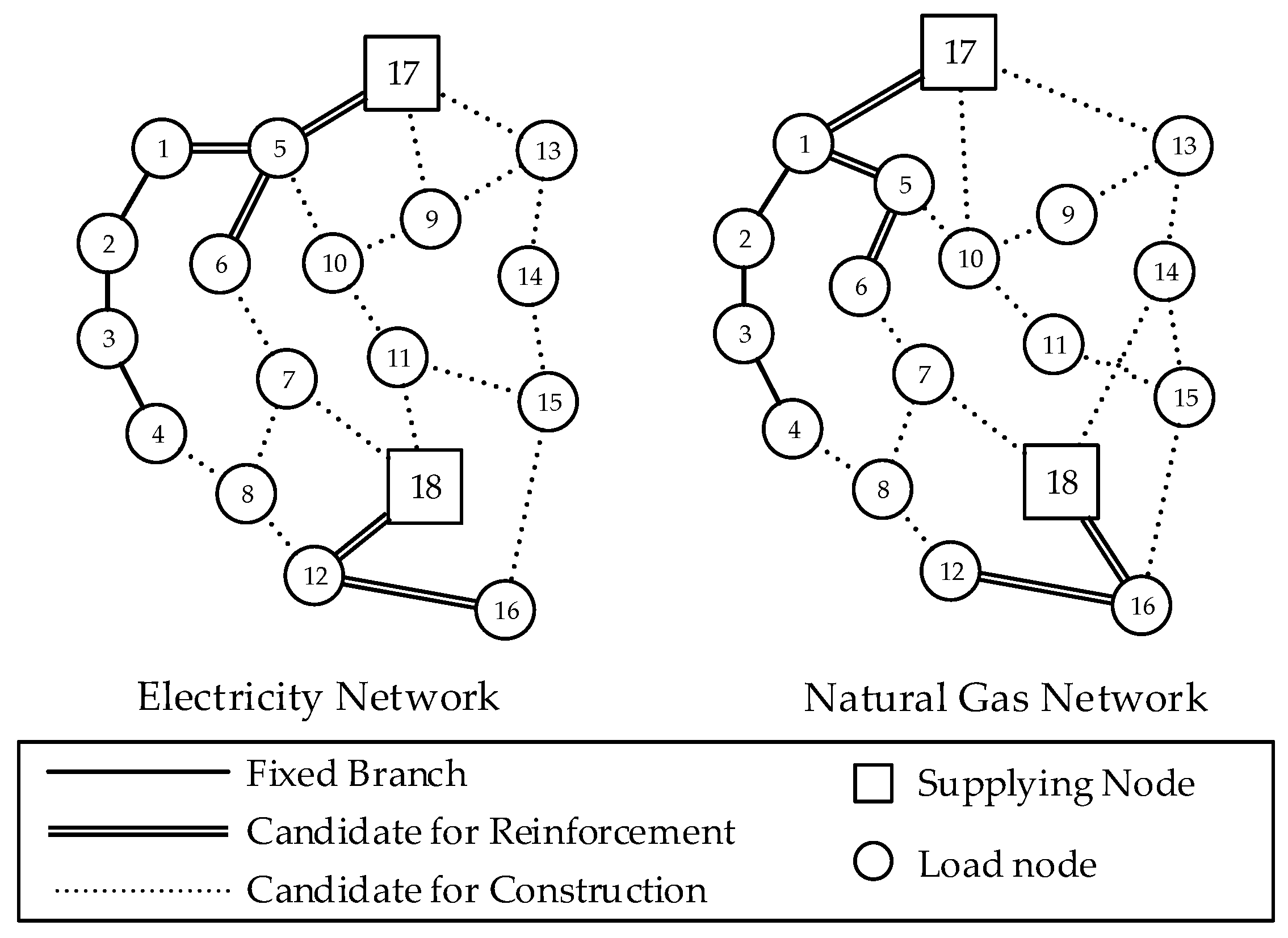
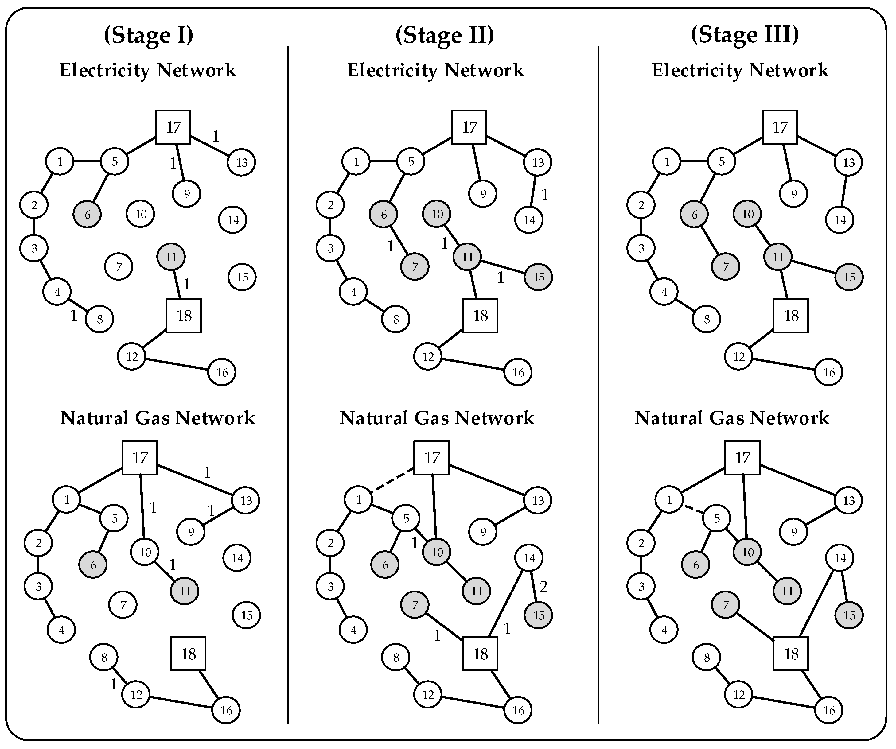
This model is nonlinear due to the gas flow equations through pipelines, that is, (20.a)–(20.d). Since the nonlinear terms of these equations are quite similar, in the following, the linearization process of (20.a) is explained. In this way, at first, in order to eliminate the square value of nodal pressures a new set of variables are introduced, as follows:

$${\pi }_{lp,t,ll}={\lambda }_{lp,t,ll}^2$$

(29.a)

$$\left|f_{b,t,ll}-{\beta }_b\sqrt{\left|{\displaystyle {\sum }_{\mathrm{lp}\in \Xi }{\chi }_{lp,b}^{Gas}{\pi }_{lp,t,ll}}\right|}\right|\le M(1-{\phi }_{b,t}^{Pi,Fi});\hspace{1em}\forall \mathrm{b}\in {\Lambda }^f$$

(29.b)

$${\left({\lambda }^{min}\right)}^2\le {\pi }_{lp,t,ll}\le {\left({\lambda }^{max}\right)}^2$$

(30)

Then, by introducing some new positive variables and auxiliary binary variables to the model, the absolute value calculation underneath the radical sign can be omitted:

$$\left|{\widehat{f}}_{b,t,ll}-{\beta }_b\sqrt{\Delta {\pi }_{b,t,ll}}\right|\le M(1-{\widehat{\phi }}_{b,t}^{Pi,Fi});\hspace{1em}\forall \mathrm{b}\in {\Lambda }^f$$

(31.a)

$$\left|{{\widehat{f}}^{\prime }}_{b,t,ll}-{\beta }_b\sqrt{\Delta {\pi }_{b,t,ll}}\right|\le M(1-{{\widehat{\phi }}^{\prime }}_{b,t}^{Pi,Fi});\hspace{1em}\forall \mathrm{b}\in {\Lambda }^f$$

(31.b)

$$\left|\Delta {\pi }_{b,t,ll}-{\displaystyle {\sum }_{\mathrm{lp}\in \Xi }{\chi }_{lp,b}^{Gas}{\pi }_{lp,t,ll}}\right|\le M(1-{\widehat{\phi }}_{b,t}^{Pi,Fi});\hspace{1em}\forall \mathrm{b}\in {\Lambda }^f$$

(31.c)

$$\left|\Delta {\pi }_{b,t,ll}+{\displaystyle {\sum }_{\mathrm{lp}\in \Xi }{\chi }_{lp,b}^{Gas}{\pi }_{lp,t,ll}}\right|\le M(1-{{\widehat{\phi }}^{\prime }}_{b,t}^{Pi,Fi});\hspace{1em}\forall \mathrm{b}\in {\Lambda }^f$$

(31.d)

$${\widehat{\phi }}_{b,t}^{Pi,Fi}+{{\widehat{\phi }}^{\prime }}_{b,t}^{Pi,Fi}\le 1; \forall \mathrm{b}\in {\Lambda }^f$$

(31.e)

$${\phi }_{b,t}^{Pi,Fi}={\widehat{\phi }}_{b,t}^{Pi,Fi}+{{\widehat{\phi }}^{\prime }}_{b,t}^{Pi,Fi}; \forall \mathrm{b}\in {\Lambda }^f$$

(31.f)

$$f_{b,t,ll}={\widehat{f}}_{b,t,ll}- {{\widehat{f}}^{\prime }}_{b,t,ll}$$

(31.g)

$$\Delta {\pi }_{b,t,ll}, {\widehat{f}}_{b,t,ll}, {{\widehat{f}}^{\prime }}_{b,t,ll}\ge 0$$

(31.h)

note that since $\Delta {\pi }_{b,t,ll}$ is a positive variable, only one of the constraints (31.c), (31.d) can be feasible for a given in-service pipeline b, depending on the sign of the result of ${\displaystyle {\sum }_{\mathrm{lp}\in \Xi }{\chi }_{lp,b}^{Gas}{\pi }_{lp,t,ll}}$. For instance, for an in-service branch b (i.e., ${\phi }_{b,t}^{Pi,Fi}=1$), constraints (31.e) together with (31.f) express that one of the auxiliary binary variables ${\widehat{\phi }}_{b,t}^{Pi,Fi},{{\widehat{\phi }}^{\prime }}_{b,t}^{Pi,Fi}$ must be 1. Hence, if the outcome of ${\displaystyle {\sum }_{\mathrm{lp}\in \Xi }{\chi }_{lp,b}^{Gas}{\pi }_{lp,t,ll}}$ is positive, for example, ${\widehat{\phi }}_{b,t}^{Pi,Fi}$ is forced to 1 which indicates that the flow is in the predetermined direction and (31.a) becomes active so that the value of the branch flow would be assigned to ${\widehat{f}}_{b,t,ll}$. In contrast, when ${\displaystyle {\sum }_{\mathrm{lp}\in \Xi }{\chi }_{lp,b}^{Gas}{\pi }_{lp,t,ll}}$ is negative, ${{\widehat{\phi }}^{\prime }}_{b,t}^{Pi,Fi}$ takes value 1. Hence, (31.b) would be active and ${{\widehat{f}}^{\prime }}_{b,t,ll}$ represents the flow of branch b.

Consequently, Equation (21.a) must be replaced by the following equations:

$${\widehat{f}}_{b,t,ll}\le f_b^{max}{\widehat{\phi }}_{b,t}^{Pi,Fi};\hspace{1em}\forall \mathrm{b}\in {\Lambda }^f$$

(32.a)

$${\widehat{f}}_{b,t,ll}^{\prime }\le f_b^{max}{{\widehat{\phi }}^{\prime }}_{b,t}^{Pi,Fi};\hspace{1em}\forall \mathrm{b}\in {\Lambda }^f$$

(32.b)

Finally, a piecewise linear approximation can be employed to accurately calculate the square root of the pressure drop through pipelines. By doing so, Equations (31.a,b) are rewritten as follows:

$$\left|{\widehat{f}}_{b,t,ll}-{\beta }_b{\displaystyle {\sum }_{i=1}^{N_{pln}}{\gamma }_i\Delta {\pi }_{b,t,ll}^i}\right|\le M(1-{\widehat{\phi }}_{b,t}^{Pi,Fi});\hspace{1em}\forall \mathrm{b}\in {\Lambda }^f$$

(33.a)

$$\left|{{\widehat{f}}^{\prime }}_{b,t,ll}-{\beta }_b{\displaystyle {\sum }_{i=1}^{N_{pln}}{\gamma }_i\Delta {\pi }_{b,t,ll}^i}\right|\le M(1-{{\widehat{\phi }}^{\prime }}_{b,t}^{Pi,Fi});\hspace{1em}\forall \mathrm{b}\in {\Lambda }^f$$

(33.b)

$$\Delta {\pi }_{b,t,ll}={\displaystyle {\sum }_{i=1}^{N_{pln}}\Delta {\pi }_{b,t,ll}^i}$$

(33.c)

$$0\le \Delta {\pi }_{b,t,ll}^i\le \Delta {\pi }^{i,\max }$$

(33.d)

where, N_pln is the number of blocks of piecewise linear pipeline flow function. Now, we have reached a linear model for co-planning study of a multicarrier energy system which can be efficiently solved using available commercial optimization software packages.

4. Case Study

In this section, the proposed co-expansion planning model is applied to a typical multicarrier energy distribution system. As shown in Figure 3, this energy system comprises electricity and natural gas networks, each consisting of 18 nodes: 16 load nodes and 2 supplying nodes (i.e., substation node for electricity network and city gate node for natural gas network). Moreover, two and three alternatives are considered for reinforcement and construction of candidate branches, respectively. The gas flow equations are also approximated by a piecewise linear function comprising four segments. As in Reference [28], the planning horizon is four years which is divided to three stages: duration of the first two is one year, while the third stage is two-year long. Furthermore, three load levels are considered as peak, medium and low load periods, with durations of 1000, 5760 and 2000 h, respectively. The whole model was implemented in General Algebraic Modelling System (GAMS) environment and solved by CPLEX solver, version 12.6.3 on a Fujitsu Celsius W530 POWER with a Quad 3.30 GHz Intel Xenon E3-1230 processor and 32 GB of RAM. The optimal gap tolerance was also set to 1%. It is worth mentioning that all the input data are available from [33].

Running the proposed MILP model of co-expansion studies, the optimal network topologies depicted in Figure 4, are obtained. In this figure, indices of the selected alternatives are placed alongside the candidate branches. For instance, label of the branch between nodes 13 and 17, at the first stage of electricity network, implies that the first alternative for construction of this feeder should be chosen. Accordingly, four feeders must be added at the first stage and four new feeders are required at the second stage. Moreover, the natural gas network needs five and four new pipelines at the first and second stages, respectively. Note that the dashed lines between nodes 17 and 1 at the second stage and nodes 1 and 5 at the third stage of gas network represent the unused pipelines to satisfy constraints regarding the radial operation of natural gas distribution network. The grey-shaded nodes indicate the load points at which CHP units are installed. Finally, it is worth noting that no pipeline or feeder reinforcements are required.

The investment and operating costs associated with optimal co-expansion planning studies of Case I and separate expansion planning of Case II are also illustrated in

Table 1. Comparison of Outcomes for two Cases.

Simulation Outcome		Case I	Case II
$C{\mathrm{F}}^{EH}$ (M$)	Inv.	0.686	0.689
	Op.	20.576	20.509
$C{\mathrm{F}}^{EDN}$ (M$)	Inv.	5.928	7.066
	Op.	0.002	0.002
$C{\mathrm{F}}^{GDN}$ (M$)	Inv.	8.339	8.737
	Op.	0.002	0.002
Total Cost (M$)		35,533	37,005
Total Installed CHP Capacity (MW)		1	1
Total Electricity Served by CHPs (GWh)		21.191	27.039
Total Electricity Energy from the Grid (GWh)		161.760	155.790
Total Gas from the Grid (Mm3)		31.610	32.441
Electricity Network Peak Demand (MW)		8.036	8.036
Natural Gas Network Peak Demand (m3/h)		1554.396	1554.396
CHP Nodes		6-7-10-11-15	1-4-5-6-8-13-16
Simulation Time (s)		477.64	74.69

. According to this table, Case II in which the EH, electricity and gas distribution expansion planning studies are carried out separately, results in a lower EH cost than Case I. However, in case of co-expansion planning, this increment is dominated with the networks expansion costs reduction so that a lower cost solution is obtained, despite the fact that the values of peak demand for both networks have not changed. It is worth noting that in both cases, due to the cost-effectiveness, total capacity of installed CHP units is at the maximum value determined by (4.d).

Nevertheless, as can be seen from the table, the selected load points for installation of CHP units are considerably different. Moreover, as illustrated in Table 1, in collaborative expansion planning mode (Case I), the energy production of CHP units as well as total energy demand of gas network are reduced. In fact, in separate planning regime (Case II), EH owner tends to install CHP units at higher number of load points in order to locally serve heat demands at lower costs. However, it causes the injection of electricity power generated by CHP units at more diverse nodes, which calls for providing more electricity network capacity to handle it. At the same time, in comparison with Case I, more investment should be made in natural gas network to be able to serve increased gas demand (owing to the natural gas consumption of CHP units) at such nodes. Therefore, optimizing the EHs objective, without considering its impact on the distribution infrastructures, results in the increased investment costs of both electricity and natural gas networks. However, comparing the obtained results of the investigated cases, it can be inferred that this is not efficient from the viewpoint of social welfare.

Finally, as can be expected, solving the integrated planning model (Case I) needs considerably more running time as seen in Table 1. The full test system database and detailed results are also available from [33].

5. Conclusions

In this paper, a new framework has been proposed for expansion co-planning studies of natural gas and electricity distribution networks. In this regard, the concept of energy hub is employed to effectively model the interactions of different energy carriers. Extracting the mathematical model of co-planning problem, an effective algorithm has been introduced to reach a MILP model for this problem. The proposed framework was applied to a multi-carrier energy test system and the achieved results were illustrated and compared with traditional separate planning studies. Lowering the required investment for expansion of distribution networks and optimizing the future vision of EHs based on operating conditions of energy networks are superiorities of the co-planning studies compared to separate planning studies.

References

1. Zhang, Y.; He, Y.; Yan, M.; Guo, C.; Ding, Y. Linearized Stochastic Scheduling of Interconnected Energy Hubs Considering Integrated Demand Response and Wind Uncertainty. Energies 2018, 11, 2448. [Google Scholar] [CrossRef]
2. Chaudry, M.; Jenkins, N.; Strbac, G. Multi-time period combined gas and electricity network optimization. Electr. Power Syst. Res. 2008, 78, 1265–1279. [Google Scholar] [CrossRef]
3. Zhang, X.; Che, L.; Shahidehpour, M.; Alabdulwahab, A.; Abusorrah, A. Electricity-natural gas operation planning with hourly demand response for deployment of flexible ramp. IEEE Trans. Sustain. Energy 2016, 7, 996–1004. [Google Scholar] [CrossRef]
4. Chen, S.; Wei, Z.; Sun, G.; Cheung, K.W.; Sun, Y. Multi-linear probabilistic energy flow analysis of integrated electrical and natural-gas systems. IEEE Trans. Power Syst. 2017, 32, 1970–1979. [Google Scholar] [CrossRef]
5. Chen, S.; Wei, Z.; Sun, G.; Wang, D.; Zhang, Y.; Ma, Z. Stochastic look-ahead dispatch for coupled electricity and natural-gas networks. Electr. Power Syst. Res. 2018, 164, 159–166. [Google Scholar] [CrossRef]
6. Costa, D.C.; Nunes, M.V.; Vieira, J.P.; Bezerra, U.H. Decision tree-based security dispatch application in integrated electric power and natural-gas networks. Electr. Power Syst. Res. 2016, 141, 442–449. [Google Scholar] [CrossRef]
7. Unsihuay-Vila, C.; Marangon-Lima, J.W.; de Souza, A.C.Z.; Perez-Arriaga, I.J.; Balestrassi, P.P. A model to long-term, multiarea, multistage, and integrated expansion planning of electricity and natural gas systems. IEEE Trans. Power Syst. 2010, 25, 1154–1168. [Google Scholar] [CrossRef]
8. Qiu, J.; Dong, Z.Y.; Zhao, J.H.; Xu, Y.; Zheng, Y.; Li, C.; Wong, K.P. Multi-stage flexible expansion co-planning under uncertainties in a combined electricity and gas market. IEEE Trans. Power Syst. 2015, 30, 2119–2129. [Google Scholar] [CrossRef]
9. He, C.; Wu, L.; Liu, T.; Shahidehpour, M. Robust co-optimization scheduling of electricity and natural gas systems via ADMM. IEEE Trans. Sustain. Energy 2017, 8, 658–670. [Google Scholar] [CrossRef]
10. Chen, S.; Wei, Z.; Sun, G.; Cheung, K.W.; Wang, D. Identifying optimal energy flow solvability in electricity-gas integrated energy systems. IEEE Trans. Sustain. Energy 2017, 8, 846–854. [Google Scholar] [CrossRef]
11. Zhang, X.; Che, L.; Shahidehpour, M.; Alabdulwahab, A.S.; Abusorrah, A. Reliability-based optimal planning of electricity and natural gas interconnections for multiple energy hubs. IEEE Trans. Smart Grid 2017, 8, 1658–1667. [Google Scholar] [CrossRef]
12. Zhang, X.; Shahidehpour, M.; Alabdulwahab, A.; Abusorrah, A. Optimal expansion planning of energy hub with multiple energy infrastructures. IEEE Trans. Smart Grid 2015, 6, 2302–2311. [Google Scholar] [CrossRef]
13. Dongxiao, W.; Jing, Q.; Ke, M.; Xiaodan, G.; Zhaoyang, D. Coordinated expansion co-planning of integrated gas and power systems. J. Mod. Power Syst. Clean Energy 2017, 5, 314–325. [Google Scholar]
14. Saldarriaga, C.A.; Hincapié, R.A.; Salazar, H. A holistic approach for planning natural gas and electricity distribution networks. IEEE Trans. Power Syst. 2013, 28, 4052–4063. [Google Scholar] [CrossRef]
15. Odetayo, B.; MacCormack, J.; Rosehart, W.D.; Zareipour, H. A chance constrained programming approach to integrated planning of distributed power generation and natural gas network. Electr. Power Syst. Res. 2017, 151, 197–207. [Google Scholar] [CrossRef]
16. Pazouki, S.; Mohsenzadeh, A.; Ardalan, S.; Haghifam, M.R. Optimal place, size, and operation of combined heat and power in multi carrier energy networks considering network reliability, power loss, and voltage profile. IET Gener. Trans. Distrib. 2016, 10, 1615–1621. [Google Scholar] [CrossRef]
17. Geidl, M.; Koeppel, G.; Favre-Perrod, P.; Klockl, B.; Andersson, G.; Frohlich, K. Energy hubs for the future. IEEE Power Energy Mag. 2007, 5, 24–30. [Google Scholar] [CrossRef]
18. Parisio, A.; Del Vecchio, C.; Vaccaro, A. A robust optimization approach to energy hub management. Int. J. Electr. Power Energy Syst. 2012, 42, 98–104. [Google Scholar] [CrossRef]
19. Moeini-Aghtaie, M.; Farzin, H.; Fotuhi-Firuzabad, M.; Amrollahi, R. Generalized analytical approach to assess reliability of renewable-based energy hubs. IEEE Trans. Power Syst. 2017, 32, 368–377. [Google Scholar] [CrossRef]
20. Barmayoon, M.H.; Fotuhi-Firuzabad, M.; Rajabi-Ghahnavieh, A.; Moeini-Aghtaie, M. Energy storage in renewable-based residential energy hubs. IET Gener. Trans. Distrib. 2016, 10, 3127–3134. [Google Scholar] [CrossRef]
21. Wong, S.; Bhattacharya, K.; Fuller, J.D. Electric power distribution system design and planning in a deregulated environment. IET Gener. Trans. Distrib. 2009, 3, 1061–1078. [Google Scholar] [CrossRef]
22. Jooshaki, M.; Abbaspour, A.; Fotuhi-Firuzabad, M.; Moeini-Aghtaie, M.; Lehtonen, M. Incorporating the effects of service quality regulation in decision-making framework of distribution companies. IET Gener. Trans. Distrib. 2018, 12, 4172–4181. [Google Scholar] [CrossRef]
23. Humayd, A.S.B.; Bhattacharya, K. Distribution system planning to accommodate distributed energy resources and PEVs. Electr. Power Syst. Res. 2017, 145, 1–11. [Google Scholar] [CrossRef]
24. Muñoz-Delgado, G.; Contreras, J.; Arroyo, J.M. Joint expansion planning of distributed generation and distribution networks. IEEE Trans. Power Syst. 2015, 30, 2579–2590. [Google Scholar] [CrossRef]
25. Li, R.; Wang, W.; Chen, Z.; Jiang, J.; Zhang, W. A review of optimal planning active distribution system: Models, methods, and future researches. Energies 2017, 10, 1715. [Google Scholar] [CrossRef]
26. Kazmi, S.; Shahzad, M.; Shin, D. Multi-objective planning techniques in distribution networks: A composite review. Energies 2017, 10, 208. [Google Scholar] [CrossRef]
27. Lotero, R.C.; Contreras, J. Distribution system planning with reliability. IEEE Trans. Power Deliv. 2011, 26, 2552–2562. [Google Scholar] [CrossRef]
28. Haffner, S.; Pereira, L.F.A.; Pereira, L.A.; Barreto, L.S. Multistage model for distribution expansion planning with distributed generation—Part I: Problem formulation. IEEE Trans. Power Deliv. 2008, 23, 915–923. [Google Scholar] [CrossRef]
29. Pereira Junior, B.R.; Cossi, A.M.; Contreras, J.; Sanches Mantovani, J.R. Multiobjective multistage distribution system planning using tabu search. IET Gener. Trans. Distrib. 2014, 8, 35–45. [Google Scholar] [CrossRef]
30. Bollobás, B. Modern Graph Theory; Springer Science & Business Media: New York, NY, USA, 2013; pp. 8–14. [Google Scholar]
31. Heidari, S.; Fotuhi-Firuzabad, M.; Kazemi, S. Power distribution network expansion planning considering distribution automation. IEEE Trans. Power Syst. 2015, 30, 1261–1269. [Google Scholar] [CrossRef]
32. Lavorato, M.; Franco, J.F.; Rider, M.J.; Romero, R. Imposing radiality constraints in distribution system optimization problems. IEEE Trans. Power Syst. 2012, 27, 172–180. [Google Scholar] [CrossRef]
33. Input Data and Results. Available online: https://drive.google.com/open?id=1eaqZSbXYtvWJbeS2Qcg7XmUeW0CU7brs. (accessed on 15 January 2019).
Figure 1. The proposed co-expansion planning framework.
Energies 12 01020 g001
Figure 2. Structure of the proposed energy hub.
Energies 12 01020 g002
Figure 3. Diagram of the electricity and natural gas distribution networks.
Energies 12 01020 g003
Figure 4. Optimal networks topologies at each stage.
Energies 12 01020 g004