Comparative Analysis of Adjustable Robust Optimization Alternatives for the Participation of Aggregated Residential Prosumers in Electricity Markets

Abstract

Active participation of end users in energy markets is identified as one of the major challenges in the energy transition context. One option to bridge the gap between customers and the market is aggregators of smart homes or buildings. This paper presents an optimization model from the standpoint of an aggregator of residential prosumers who have PV panels, electric water heaters, and batteries installed at home level. This aggregator participates in the day-ahead energy market to minimize operation costs by controlling the settings of flexible devices. Given that energy prices, PV production, and demand have uncertain behavior, appropriate models should be used to include these effects. In the present work, Adjustable Robust Optimization (ARO) is used to include uncertainty in the optimization model, and a comparative study of modifications to this formulation is carried out to determine its potential and limitations. The comparative analysis is performed from the point of view of average cost and risk, after performing Monte Carlo simulation. Simulations show the advantages of using an ARO framework when compared to deterministic approaches and also allow us to conclude about the advantages of using the proposed alternative formulation to find more attractive solutions for an aggregator.

1. Introduction

1.1. Overview

The energy transition requires a series of efforts by industry, governments, and citizens in general. One of the main challenges of reaching decarbonization goals is the transformation of electrical systems. In an attempt to achieve this, the number of large renewable power plants has increased in recent years. In addition, energy storage systems and demand side management play an important role to support decisions made by the multiple actors in the system. In the case of distributed energy resources, management of devices is also important to locally offset variation in load or Renewable Energy Sources (RES) and to achieve minimum-cost operation. In addition, the presence of microgrids (MG) in lower layers of the distribution grid, in the form of aggregated smart building/homes or energy communities, makes it possible for demand side management and energy storage systems to support operational decisions and to increase/decrease profit/cost when market rules permit trading of flexibility services on wholesale, ancillary, or local markets.

Despite the recent development of decentralized renewable generation and control possibilities, there is still a lack of models, market rules, and frameworks to provide flexibility in the lower layers of the grid. At medium and Low Voltage (LV) levels, along with the key role played by energy storage in flexible grid operation, the aggregation of resources at the building and home level is crucial to ensure the portfolio optimization of different actors while providing flexibility [1].

European authorities have highlighted the importance of promoting consumer participation in energy markets by creating the necessary marketplaces or by removing market barriers to enable the participation of local energy communities [2]. This stimulation of consumers in order to put them at the center of the energy market can be done from individual participation standpoints or by aggregated mechanisms. This change of paradigm allows consumers to increase the integration of local generation for self-consumption and market participation, so that they become prosumers. Given that direct participation of prosumers still encounters barriers, aggregators appear as an option to bridge the gap. In addition, new mathematical optimization models need to account for uncertainty, which also brings additional complexity to the decision-making process.

1.2. Literature Review

Several research papers have concluded on and recommended the importance of including uncertainty in a smart grid context [3,4]. For instance, to bid properly in day-ahead energy markets, some knowledge about the next day’s prices is required to hedge risk. In addition, uncertainty about both demand and the Renewable Energy Resources (RES) installed at the residential level can lead to sub-optimal scheduling plans for residential aggregators due to the imbalances produced by the actual production and load patterns during the operation day [5,6]. This risk has to be properly quantified and embedded in decision-making on the operation and scheduling of flexibility and remains an open field of research due to the complexity of uncertainty modeling and the algorithms required to solve this type of optimization problem.

Stochastic optimization has been traditionally used for modeling uncertainty in optimization problems [7]. If a number of scenarios for the uncertain variables is found, then an equivalent optimization problem can be reformulated to obtain an expected value of the objective function based on the probability of each scenario. The trade-off is the computational effort associated with the increase in problem size [4] and the necessary statistical information to create and reduce the number of scenarios.

Robust Optimization (RO) [8] appears as an option to model uncertain behavior in optimization problems. RO defines a confidence interval for each uncertain variables and returns an immunized solution that remains feasible within this interval. In addition, RO does not require detailed probabilistic information about the uncertain variables.

Some research has recently been published on exploiting RO capabilities for handling uncertainty in medium-sized distributed energy resources and microgrids. Price uncertainty is modeled in [9,10], and RES and/or load uncertainty modeling is proposed in [11,12,13,14,15,16].

Research in the area of residential prosumer aggregation under robust approaches is still very limited. Some of the smart home-oriented approaches that have recently appeared in the specialized literature are related to electricity bill minimization [17], aggregation of storage devices in real time [18], and thermal storage at the residential level [19]. The sources of uncertainty included in each of these papers are comfort, energy prices, and thermal demand, respectively. In [19], RO is used to model uncertainty in RES and prices, in order to manage resources in an energy community.

One common critique of RO is its over-conservative solutions, given that RO in its original formulation considers all potential deviations of the uncertain coefficients. This can be countered by Adjustable Robust Optimization (ARO) [20] through the introduction of robust control parameters. In the case of medium voltage-level MG, limited analysis of these control parameters has been proposed. For the case of residential aggregators, and to the authors’ knowledge, research on the impacts of uncertainty budget is virtually inexistent.

The specialized literature has presented some models for residential aggregation with RES and storage technologies, in which different objectives are pursued, such as energy and reserve market participation [21], as well as the definition of billing systems and incentive mechanisms [22]. Uncertainty was included by means of stochastic optimization and the chance-constrained method in [21] and model predictive control in [22].

Different storage technologies and their coordination can also help provide flexibility and counter uncertainty in scheduling tasks. However, aggregation models that analyze interactions of thermal and electrochemical storage at the residential level are not commonly present in the literature. The model proposed in [23] combined thermal and electrical storage for a residential microgrid with the purpose of shaving demand peak and enhancing the system’s self-sufficiency. The day-ahead stochastic model in [24] did not consider Battery Energy Storage Systems (BESS), but featured electro-thermal storage from a retailer’s perspective. Moreover, sizing and operation of storage devices in smart buildings was presented in [25], including electrical and thermal storage. These two types of storage were also modeled in [26] to analyze cooperative schemes among smart residential buildings. The approach in [27] presented a methodology for intraday management of PV and Electric Water Heaters (EWH) in an LV network, with the EWH acting as a flexible load in order to achieve minimum operation costs.

When including electrochemical storage, unconstrained cycling patterns can lead to faster degradation of BESS and loss of life. Among the aggregation schemes currently published, few present details of storage cycling characteristics for inclusion of equivalent degradation costs, in spite of their importance in energy bidding and scheduling-related problems [28,29].

In the referenced works dealing with MG scheduling and management, the non-linear relation between Depth of Discharge (DoD) and equivalent cycling aging was neglected. In the case of [9,12,13], linear costs were assumed as a function of power charge and discharge. The proposed models were simplified and neglected DoD vs. cycle characteristic, which present highly non-linear behavior and depend on internal chemical reactions with electrode interfaces. The linear costs in [9,12,13] assumed that degradation is proportional to power charge and discharge, but no further identification of cycles and the respective DoD was proposed. This can lead to suboptimal bidding strategies and device schedules. Moreover, the works in [11,14,15] neglected cycling aging impacts.

1.3. About the Present Paper

Current recommendations to facilitate prosumers’ key role in the energy transition process emphasize promoting storage technologies and engaging consumers with aggregators so they can take active part in the electricity market. To contribute in these directions, new mathematical models have to be developed to manage optimally prosumers’ resources and exploit flexibility. In the context of these challenges, the main contributions of this work are to:

• Propose a model for market participation of prosumer aggregation including the effects of multiple sources of uncertainty, i.e., energy prices, PV production, electrical and thermal demand, and including the effects of battery degradation.
• Propose modified versions of ARO to counter conservatism for prosumer aggregation by changes in the model regarding the budget of uncertainty and comparing performance with hybrid robust/stochastic solutions.
• Present numerical results to demonstrate the advantages of the proposed modifications over deterministic formulations in terms of both operation cost and risk. These tests are performed on a home energy management system with data from a real-life demonstrator.

The present paper builds on the work presented by the authors in [30], but significantly improves, expands, and differs from the mentioned paper in several aspects: (1) We present a comparative analysis of robust optimization and a hybrid stochastic/robust approach. (2) Several alternatives of the formulation of adjustable robust optimization are presented, for instance (a) analysis of the impacts of separate uncertainty budgets for PV and electrical demand, (b) uncertainty budget manipulation to achieve higher resolution for close-to-deterministic values, and (c) comparative analysis of all alternatives from the standpoint of cost and risk. (3) Energy prices are forecasted with a kernel density estimator, and this tool is used to (a) create the confidence interval for the robust model, (b) create the scenarios for the hybrid stochastic approach, and (c) generate samples for a performance evaluation through Monte Carlo simulation. (4) Descriptors are proposed to rank the best solutions and describe the general performance of the alternatives.

The motivation of including also hybrid stochastic/robust schemes for comparison purposes lies in the fact that in real-life applications, it may not feasible to create high quality scenarios for all forecasted variables needed by the stochastic optimization approach. To generate such scenarios, one should take into account spatio-temporal correlations among the variables. For instance, creating PV and demand correlated scenarios for stochastic optimization can be a complex task and remains as an open research field, whereas defining an uncertainty interval for robust optimization is a more straightforward task, which does not necessarily need correlation analysis. In addition, suitable scenarios to model price uncertainty, independently of the available PV and demand information, can be practically created and used in stochastic optimization. The hybrid approach permits flexibility to consider probabilistic forecasts that may be provided in practical cases in different formats (i.e., in the form of scenarios or ensembles and in the form of prediction intervals).

Robust optimization to deal with prosumers’ aggregation decision-making is still rarely treated in the specialized literature. Moreover, no previous works have analyzed the potential and limitations of alternatives for uncertainty treatment as proposed in this work. Additionally, the present research is part of the EU Horizon 2020 project Storage-Enabled Sustainable Energy for Buildings and Communities (SENSIBLE), and belongs to the particular case “flexibility and demand side management in market participation”. This case assumes an agent that aggregates residential customers and participates in a market to add value to their flexibility.

The paper is organized as follows: Section 2 sets out the framework of the proposed model and the deterministic formulation of the optimization problem. Next, Section 3 develops the robust counterpart and alternative ARO formulations. Section 4 presents the comparative results and analysis of the proposed approach, and concluding remarks are outlined in Section 5.

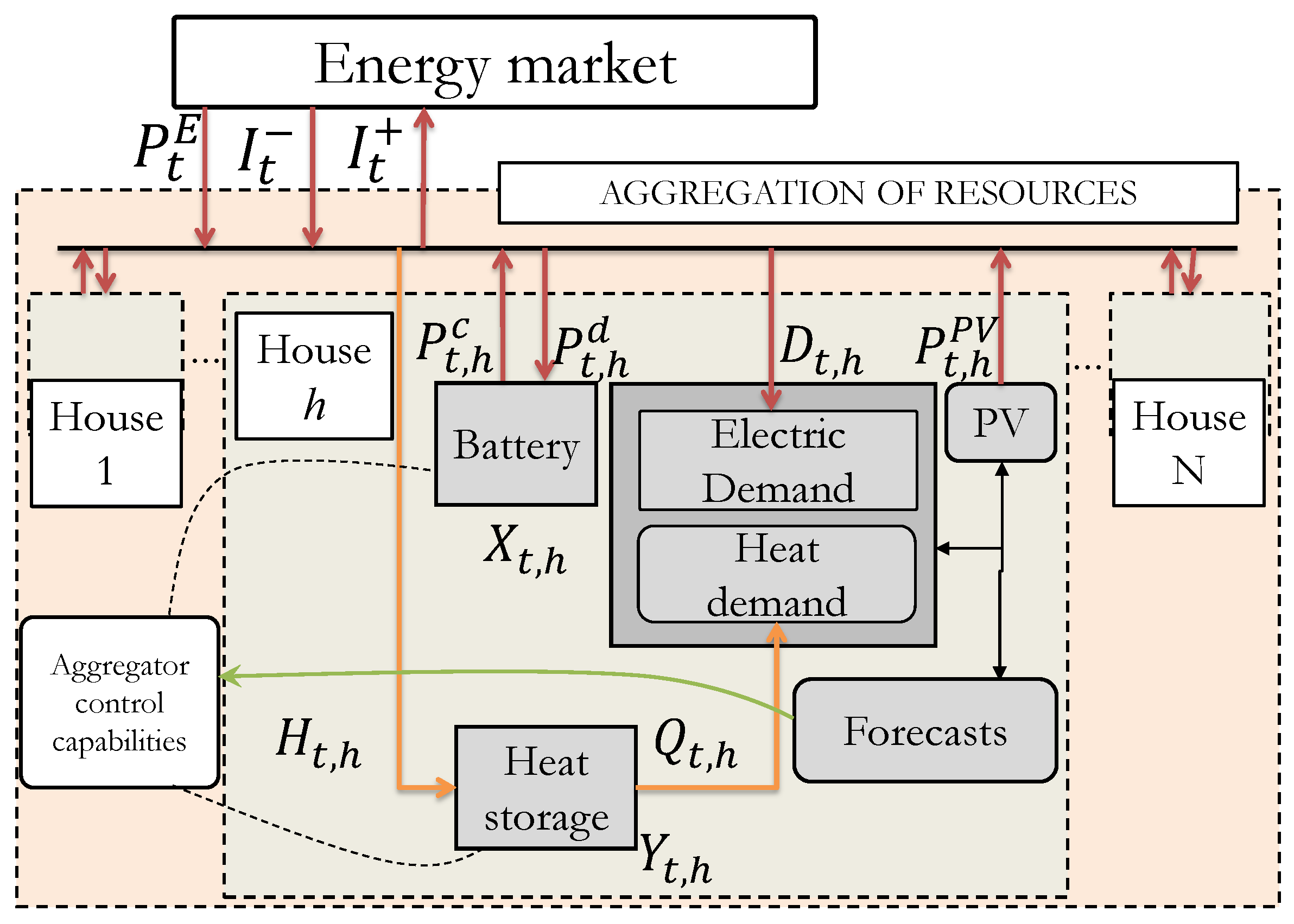
2. Framework and Mathematical Model

The proposed framework assumes a number of households with PV panels, EWH, and BESS. These devices can be controlled by an entity called the aggregator. This aggregator schedules devices by controlling set-points and participates in the day-ahead energy market, with the purpose of achieving minimum operation costs and considering the inherent degradation of the BESS installed in the households. A schematic diagram of the proposed prosumer aggregation is shown in Figure 1.

In this proposal, heat demand ($Q_{t,h}$) is directly met by the heat storage device (an EWH). The heat demand is met by available stored energy in the Thermal Energy Storage (TES), $Y_{t,h}$, and its associated input is $H_{t,h}$. This can be seen as a flexible load, which, depending on the opportunity cost captured by the optimization model, responds by storing hot water even if it is not immediately used by the occupants.

With the aggregation of resources to participate in day-ahead energy markets, the deterministic optimization problem is presented next.

2.1. Objective Function

The present deterministic model supposes an aggregator of residential flexibility that participates in the day-ahead energy market by controlling the set-points over a predefined horizon of 24-h (T) time-steps. The objective function aims to minimize energy purchases in the wholesale market and overall operational costs. This model takes into account day-ahead energy prices (${\pi }_t$) and the possibility of purchasing or selling energy ($P_t^E$) at the Point of Common Coupling (PCC). In addition, the aggregator offsets day-ahead purchase deviations with actual generation and demand levels, by participating in the imbalance market, where $I_t^{-}$ ($I_t^{+}$) indicates additional imports (exports) in real time. The present model supposes that energy requirements or surplus at the PCC can be traded in the wholesale market without market or regulation barriers. These interactions are shown in the objective function (1), in which the decision is associated with:

• ${\displaystyle \sum _{t=1}^T}{\pi }_t{P}_t^E$: the cost of the day-ahead traded energy with the wholesale market.
• ${\displaystyle \sum _{t=1}^T}{\mu }_t^{-}{I}_t^{-}-{\mu }_t^{+}{I}_t^{+}$: the cost of purchasing additional blocks of energy (negative imbalance) and the prices received for selling surplus energy (positive imbalance) due to deviations with respect to the day-ahead committed energy. Imbalance prices presume an indirect penalization given that they are less attractive than settled day-ahead prices.
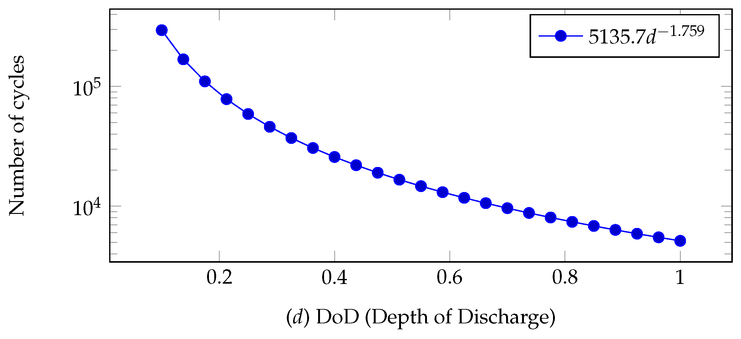
• ${\displaystyle \sum _{h=1}^N}{f}_h^{cyc}(·)$: cycling or equivalent degradation cost of the batteries in each household h. This cost is a function of the SOC vector (${\mathbf{X}}_h={[X_{1,h},\dots ,X_{1,T}]}^{\prime }$), i.e., the SOC of each battery during the day-ahead operation time horizon, provided that the SOC represents the cycling pattern.

Subscripts t and h index time-step and household, respectively. Parameters ${\pi }_t$, ${\mu }_t^{-}$, $-{\mu }_t^{+}$ represent, respectively, spot price, negative imbalance cost, and positive imbalance cost.

$$\mathrm{minimize}{\displaystyle \sum _{t=1}^T}({\pi }_t{P}_t^E+{\mu }_t^{-}{I}_t^{-}-{\mu }_t^{+}{I}_t^{+})+{\displaystyle \sum _{h=1}^N}{f}_h^{cyc}({\mathbf{X}}_h)$$

(1)

The last term in the objective function is non-linear. This term includes the corresponding non-linearities associated with chemical reactions occurring in the batteries due to temperature changes. The alternative for including degradation is expanded in Section 2.5.

2.2. Load Balance Constraints

The power balance of the aggregation is modeled by Constraint (2) and also contains the physical exchange at the Point of Common Coupling (PCC).

$$P_t^E+I_t^{-}-I_t^{+}+\Delta t{\displaystyle \sum _{h=1}^H}{P}_{t,h}^{net}=0,\forall t$$

(2)

$$P_{t,h}^{net}=P_{t,h}^{PV}-P_{t,h}^c+P_{t,h}^d-D_{t,h}-H_{t,h},\forall t,\forall h$$

(3)

$$0\le P_{t,h}^{PV}\le P_{t,h}^{P{V}_{max}},\forall t,\forall h$$

(4)

In Constraint (3), the net power in each household includes the battery charging ($P_{t,h}^c$) and discharging ($P_{t,h}^d$), the PV injection ($P_{t,h}^{PV}$), the electrical load ($D_{t,h}$), and the power input of the EWH ($H_{t,h}$). In addition, if a household is not provided with an EWH that has storage capabilities, the variable H becomes the same thermal load.

2.3. BESS Constraints

The energy state of BESS is described by Constraints (5)–(10). Binary variables $u_{t,h,s}$ and $v_{t,h,s}$ avoid simultaneous charging and discharging. Hence, a mixed integer characteristic is introduced by Constraints (7)–(9). Constraint (6) ensures the continuity of the SOC.

$$X_{t,h}=X_{t-1,h}+{\eta }^c\Delta t{P}_{t-1,h}^c-\Delta t{P}_{t-1,h}^d/{\eta }^d,\forall t,t\ne 1,\forall h,$$

(5)

$$X_{1,h}=X_{T,h},\forall h$$

(6)

$$u_{t,h}+v_{t,h}\le 1,\forall t,\forall h$$

(7)

$$0\le P_{t,h}^c\le {\overline{P}}_h^c·u_{t,h},\forall t,\forall h$$

(8)

$$0\le P_{t,h}^d\le {\overline{P}}_h^d·v_{t,h},\forall t,\forall h$$

(9)

$${{\displaystyle \underline{X}}}_h\le X_{t,h}\le {\overline{X}}_h,\forall t,\forall h$$

(10)

2.4. TES Constraints

When the EWH present in a house has storage capabilities, then it is denoted as a TES device. In this case, it is assumed that the device can be operated for immediate hot water use or for storing heat for later use in order to comply with user’s expected thermal demand ($Q_{t,h}$). The energy state ($Y_{t,h}$) is represented by the intertemporal Constraint (11). Given that TES is capable of heating water for direct consumption (shower, appliances, etc.) or for space heating for upcoming hours, energy dissipation is included in the model by R and C (thermal resistance and capacitance, respectively) in Equation (11), in line with [24].

$$Y_{t,h}=Y_{t-1,h}+\Delta t{H}_{t-1,h}-Y_{t-1,h}/R_h{C}_h-\Delta t{Q}_{t-1,h},\forall t,t\ne 1,\forall h$$

(11)

$$Y_{1,h}=Y_{T,h},\forall h$$

(12)

$${{\displaystyle \underline{Y}}}_{t,h}\le Y_{t,h}\le {\overline{Y}}_{t,h},\forall t,\forall h$$

(13)

$$0\le H_{t,h}\le {\overline{H}}_{t,h},\forall t,\forall h$$

(14)

When the EWH has no storage or control capabilities, losses in the inter-temporal constraint are neglected, as well as the thermal state of charge; hence, $H_{t,h}$ takes the value of the thermal demand ($Q_{t,h}$), which can be easily verified by Equation (11). In other words, in the absence of TES, the total load to be supplied to each house is determined by adding the electrical and thermal loads.

Equation (12) ensures continuity of the thermal storage, and Equations (13) and (14) are respectively the energy boundaries and the power of the TES device.

This formulation allows the EWH to act as a flexible load, given that power input can be controlled to capture the opportunity cost to achieve overall cost minimization while taking advantage of the storage capabilities for complying with thermal demand needs.

The deterministic Mixed-Integer Linear Programming (MILP) problem in Equations (1)–(14) combines three types of flexibility to be managed by an aggregator, i.e., PV production, electrochemical storage and thermal storage. The result of this optimization returns the set-points of all devices and the energy exchanged with the wholesale market in order to achieve a minimum operation cost for the portfolio, while complying with electrical and thermal demand in each house.

2.5. Battery Degradation Costs

For a given DoD (d), the maximum charge/discharge cycles a battery can achieve, is given by [31]:

$$n_d=n_{100}{d}^{-k_p}$$

(15)

where $k_p$ is a constant that results from curve fitting and is a function of the lifecycle versus DoD curve provided by the battery manufacturer, and $n_{100}$ corresponds to the equivalent number of cycles before failure at $d=100\%$. An example of a fitted curve for a 3-kW/3.3-kWh battery is depicted in Figure 2.

For a specific pattern of State of Charge (SOC) (vector $\mathbf{X}$), equivalent half or full cycles can be found, and an equivalent degradation cost can be obtained with the equation:

$$f^{cyc}(\mathbf{X})=C_{cyc}(d_j)={\displaystyle \sum _{j\in \Omega }}{L}_j\frac{C_{ini}}{n_{100}}{d}_j^{k_p}$$

(16)

where $\Omega$ is the set of DoDs at which each cycle occurs and $C_{ini}$ is the initial cost of the battery. The full- or half-cycle information for each $d_j$ is given by $L_j$. The obtained $C_{cyc}$ is the corresponding cost due to the battery’s aging process. This is a measure of the battery’s operational cost and is useful for bidding more accurate quantities in energy markets.

The motivation for linearizing the cost characteristic lies in the fact that if the DoDs at which each cycle occurs can be identified by means of a set of equations, then an equivalent cycling cost can be determined in such a way that these equations can be explicitly modeled and fed into a commercial optimization solver. This subsection presents an option to introduce a set of equations that capture and identify charging cycles by means of auxiliary variables and constraints, also known as special ordered sets.

The idea of the explicit modeling is to identify the beginning of each charging cycle with Constraint (17). This constraint detects the transition between an idle or charging state in $t-1$ to a charging state in t. If this is the case, variable $x_{t-1,h}=1$ and captures the time-step prior to charging mode. This transition detection is possible given that binary variable $u_{t,h}$ identifies when the battery is in charging mode. $y_{t-1,h}$ equals zero when no change in state occurs, or −1 if the battery stops charging. Constraint (19) ensures a mutually-exclusive unitary value for the special ordered sets.

In general, Equation (17) can take three possible values, i.e., 0, −1, or 1. The zero value means that $u_{t,h}=u_{t-1,h}$, which can also have four interpretations: (a) the battery is in charging mode for both $t-1$ and t; (b) the battery is in idle mode in both time-steps; (c) the battery is going from idle to discharging; or (d) the battery is going from discharging to idle. Second, if Constraint (17) equals −1, this means that $u_{t,h}=0$ and $u_{t-1,h}=1$, which means that the battery is charging in $t-1$ and is going into discharging or idle mode. Third, if Equation (17) takes the value of one, this is interpreted as a change from idle/discharging to charging mode. This latter situation is the one that interests us, given that the proposed approach intends to identify only the beginning of charging cycles.

$$x_{t-1,h}-y_{t-1,h}=u_{t,h}-u_{t-1,h},\forall t,t\ne 1,\forall h$$

(17)

$$x_{T,h}-y_{T,h}=u_{0,h}-u_{T,h},\forall h$$

(18)

$$x_{t,h}+y_{t,h}\le 1,x_{t,h},y_{t,h}\in \left\{0,1\right\},\forall t,\forall h$$

(19)

Constraint (21) is introduced so that $X^D$ stores a value different from zero for the time-step previous to the beginning of a charging cycle. Constraint (20) allows assigning the proper value of DoD. $X^{Df}$ is a slack variable that helps balance the equation in the absence of a charging cycle ($x_{t,h}=0$) and activated through Constraint (22). Note that when $x_{t,h}=0$, no DoD needs to be identified because no beginning of the charging cycle has taken place; hence, per Equation (21), $X^D=0$, and additionally, $X^{Df}$ takes the value of the current DoD, but this DoD has no impact on cycling cost calculation, as expected, given that is does not correspond to the beginning of a charging cycle.

$$X_{t,h}^D+X_{t,h}^{Df}=1-X_{t,h}/E_h^{rated},\forall t,\forall h$$

(20)

$$X_{t,h}^D\le x_{t,h},\forall t,\forall h$$

(21)

$$X_{t,h}^{Df}\le 1-x_{t,h},\forall t,\forall h$$

(22)

Note that conflicting definitions of DoD exist in the literature. The present study takes the definition of DoD as the energy discharged compared to 100% SOC.

Once each charging cycle and the associated DoD ($X^D$) are extracted, the segment of the linearized cost curve is identified by using Constraints (23)–(25). Constraint (24) forces the DoD to lie in the appropriate segment and activates a binary variable $l_{t,h,s}$ for the active segment s.

$${\displaystyle \sum _{s=1}^S}{X}_{t,h,s}^{Ds}=X_{t,h}^D,\forall t,\forall h$$

(23)

$$l_s^{min}{l}_{t,h,s}\le X_{t,h,s}^{Ds}\le l_s^{max}{l}_{t,h,s},l_{t,h,s}\in \left\{0,1\right\} \forall t,\forall h$$

(24)

$${\displaystyle \sum _{s=1}^S}{l}_{t,h,s}=x_{t,h},\forall t,\forall h$$

(25)

One difference between this approach and other models [32,33] is that $l_{t,h,s}$ is used in the objective function (26) to activate parameter $b_{h,s}$ when needed. Similarly, $X_{t,h,s}^{Ds}$ is used as the independent variable of the aging cost function.

Quantities $a_{h,s}$ and $b_{h,s}$ in (26) correspond to the piece-wise approximation parameters of the cycling aging cost.

With this reformulated calculation of the aging cost, the objective Function (1) can be re-written as:

$$\mathrm{minimize}{\displaystyle \sum _{t=1}^T}\left\{{\pi }_t{P}_t^E+{\mu }_t^{-}{I}_t^{-}-{\mu }_t^{+}{I}_t^{+}+{\displaystyle \sum _{h=1}^N}{\displaystyle \sum _{s=1}^S}(a_{h,s}{X}_{t,h,s}^{Ds}+b_{h,s}{l}_{t,h,s})\right\}$$

(26)

The equivalent accumulated degradation cost is the fourth term in objective Function (26), and parameters $a_{h,s}$, $b_{h,s}$ are obtained by segment linearization of Equation (16).

3. Robust Counterpart

Robust optimization approaches aim to find optimal and feasible solutions over an interval of values that represent uncertainty. To find a robust counterpart of the deterministic problem, each constraint containing parameters with uncertainty has to be transformed by means of strong duality theory. When inspecting the deterministic model in (1)–(14), four sources of uncertainty are identified, i.e., prices, PV production, electrical demand and thermal demand.

The tractable robust counterpart of a deterministic problem can be found by applying the strong duality theorem, explained in detail in [34].

For the case of the objective Function (26), the cost coefficients of $P_t^E$, $I_t^{-}$, and $I_t^{+}$ present uncertainty, and the equivalent dual robust counterpart is represented by Constraints (27)–(34).

$$\begin{array}{c}{\displaystyle \sum _{t=1}^T}{\displaystyle \sum _{h=1}^N}{\displaystyle \sum _{s=1}^S}(a_{h,s}{X}_{t,h,s}^{Ds}+b_{h,s}{l}_{t,h,s})+{\displaystyle \sum _{t=1}^T}({\widehat{\pi }}_t{P}_t^E+{\widehat{\mu }}_t^{-}{I}_t^{-}-{\widehat{\mu }}_t^{+}{I}_t^{+})\\ +{\displaystyle \sum _{t=1}^T}(q_t^c+q_t^{-}+q_t^{+})+{\Gamma }^{DA}{z}^c+{\Gamma }^{-}{z}^{-}+{\Gamma }^{+}{z}^{+}\end{array}$$

(27)

$$z^c+q_t^c\ge \frac{1}{2}({\overline{\pi }}_t-{\displaystyle \underline{{\pi }_t}})y_t^c,\forall t$$

(28)

$$-y_t^c\le P_t^E\le y_t^c,\forall t$$

(29)

$$z^{-}+q_t^{-}\ge \frac{1}{2}({\overline{\mu }}_t^{-}-{{\displaystyle \underline{{\mu }_t}}}^{-})y_t^{-},\forall t$$

(30)

$$-y_t^{-}\le I_t^{-}\le y_t^{-},\forall t$$

(31)

$$z^{+}+q_t^{+}\ge \frac{1}{2}({\overline{\mu }}_t^{+}-{{\displaystyle \underline{{\mu }_t}}}^{+})y_t^{+},\forall t$$

(32)

$$-y_t^{+}\le I_t^{+}\le y_t^{+},\forall t$$

(33)

$$z^c,q_t^c,y_t^c,z^{-},q_t^{-},y_t^{-},z^{+},q_t^{+},y_t^{+}\ge 0,\forall t,\forall h$$

(34)

where $z,q_t,y_t$ are dual variables of the robust counterpart. The robust parameter ${\Gamma }^{DA}$ takes values in the range [0, T] and controls the maximum number of coefficients that can deviate from the central value. For instance, if ${\Gamma }^{DA}=T$, the solution will remain optimal and feasible for T price deviations. In other words, the solution is capable of withstanding the worst-case scenario.

Another source of uncertainty is given by PV and electrical demand in Equation (2). Both quantities can be merged into one to obtain net load for each t (PV minus load). Equations (35)–(37) show the resulting robust counterpart.

$$P_t^E+I_{t,e}^{-}-I_{t,e}^{+}+\Delta t{\displaystyle \sum _{h=1}^N}{P}_{t,h}^d-P_{t,h}^c-H_{t,h}=D_t^{net}+q_t^D+{\Gamma }_t^D{z}_t^D,\forall t,\forall e$$

(35)

$$z_t^D+q_t^D\ge \frac{1}{2}({\overline{D}}_t^{net}-{{\displaystyle \underline{D}}}_t^{net})y_t^D,\forall t$$

(36)

$$z_t^D,q_t^D\ge 0,y_t^D\ge 1,\forall t$$

(37)

where,

$$D_t^{net}=\frac{1}{2}({\overline{D}}_t^{net}+{{\displaystyle \underline{D}}}_t^{net})$$

(38)

Net load deviation is controlled by the robust parameter ${\Gamma }_t^D$ with cardinality [0,1]. For a more compact notation, subindex t is eliminated, and instead, we use ${\Gamma }^D$. Index e is associated with the scenarios for the case in which the stochastic approach is used to model price uncertainty, as explained in Section 3.1.1.

Constraint (11) contains another uncertain parameter, i.e., thermal load. The application of strong duality results in the following constraints:

$$Y_{t,s,h}=Y_{t-1,s,h}+\Delta t{H}_{t-1,s,h}-Y_{t-1,s,h}/R_h{C}_h-\Delta t({{\displaystyle \stackrel{\wedge }{Q}}}_{t-1,s,h}+q_{t-1,h}^{th}+{\Gamma }_{t-1,h}^{th}{z}_{t-1,h}^{th}),\forall t,\forall h$$

(39)

$$z_{t,h}^{th}+q_{t,h}^{th}\ge \frac{1}{2}(Q_{t,h}^{90\%}-Q_{t,h}^{10\%})y_{t,h}^{th},\forall t$$

(40)

$$z_{t,h}^{th},q_{t,h}^{th}\ge 0,y_{t,h}^{th}\ge 1,\forall t,\forall h$$

(41)

For simplicity, we eliminate the subindex $t,h$ from ${\Gamma }_{t,h}$, and instead, we assume a general parameter to control robustness in the thermal load: ${\Gamma }^{th}$. Note that ${\Gamma }^{th}\in [0,1]$. $Q_{t,h}^{10\%}$ and $Q_{t,h}^{90\%}$ represent respectively the 10% and 90% quantile forecast of thermal load.

The resulting adjustable robust counterpart (ARO) is given by:

$$\mathrm{minimize}(27)$$

(42)

$$\begin{array}{cc}\hfill \mathrm{s}.\mathrm{t}.& \\ & \mathrm{Constraints}:(5)–(10),(12)–(14),(17)–(25),(28)–(37),(39)–(41)\end{array}$$

(43)

where:

• (27): is the robust counterpart of the objective function.
• (5)–(10): are the BESS constraints.
• (12)–(14): are the EWH constraints
• (17)–(25): are the BESS cycling piece-wise linearization constraints.
• (28)–(37): are the robust counterpart constraints related to power balance and net demand uncertainty.
• (39)–(41): are the robust counterpart constraints related to thermal demand uncertainty.

This robust counterpart is a tractable MILP that can be solved with commercial optimization solvers. The budget of uncertainty is given by the combination of three parameters: ${\Gamma }^{DA}$ (= ${\Gamma }^{-}$ = ${\Gamma }^{+}$), ${\Gamma }^D$ and ${\Gamma }^{th}$. Their purpose is to control conservatism in terms of the deviations in energy prices, net load, and thermal load, respectively.

3.1. Modification Alternatives to the Original Formulation

Besides ARO for modeling price uncertainty, another option is to create multiple price scenarios and use them for stochastic optimization. These scenarios are generated based on probabilistic forecasts, as explained in Section 3.5. A high number of scenarios is initially generated in order to cover all possible situations. However, this impacts calculation time in the optimization process. It is a common practice in the literature to apply scenario reduction techniques to deal with this issue. This permits deriving a set of representative scenarios that are sufficient to represent in the optimization process. First, each scenario in the set is assigned the same probability, and afterwards, some scenarios are eliminated using a reduction technique. In this paper, when scenarios are considered to model price uncertainty, a backward reduction algorithm based on Kantorovich Distance (KD) [35] is used to eliminate scenarios, consisting of the following steps:

• Create a number of initial samples using the probabilistic price forecasts, which are based on Kernel Density Estimation (KDE), and define a target number of scenarios.
• Calculate KD for each pair of scenarios in the current set. This calculation leads to a Kantorovich Distance Matrix (KDM).
• For each scenario, identify its closest neighbor j. This can be done by identifying the lowest value in each row i of the KDM.
• For each closest neighbor j in each row i, calculate $K{D}_{i,j}\times p_e(i)$, where $p_e(i)$ is the probability of scenario i.
• From the i-position vector containing of all values of $K{D}_{i,j}\times p_e(i)$, select the lowest value. Identify scenario i.
• Eliminate scenario i, and assign a probability of i to $p_e(j)$. Update the KDM.
• Repeat Steps 3–6 until the target number of scenarios is obtained.

A graphic example of the application of this reduction technique is shown in Figure 3. In this case, a total of 100 initial price scenarios was generated (dashed lines), and the reduction technique was applied to obtain 10 representative scenarios (continuous lines).

3.1.1. Modifications Regarding Objective Function

Following robust optimization to account for uncertainty of energy prices and after obtaining the reduced scenarios and corresponding probabilities with the methodology explained in the previous subsection, a stochastic optimization problem can be formulated. In this case, the objective Function (1) and Constraint (2) have to be reformulated as follows:

$$\mathrm{minimize}{\displaystyle \sum _{e=1}^{N_e}}{p}_e{\displaystyle \sum _{t=1}^T}({\pi }_{t,e}{P}_t^E+{\mu }_{t,e}^{-}{I}_{t,e}^{-}-{\mu }_{t,e}^{+}{I}_{t,e}^{+})+{\displaystyle \sum _{h=1}^N}{f}_h^{cyc}({\mathbf{X}}_h)$$

(44)

$$P_t^E+I_{t,e}^{-}-I_{t,e}^{+}+\Delta t{\displaystyle \sum _{h=1}^H}{P}_{t,h}^{net}=0,\forall t,\forall e$$

(45)

This stochastic formulation represents an alternative to include price uncertainty in the day-ahead dispatch formulation and can be combined either with a deterministic formulation for load and PV production or with robust formulation for load and PV uncertainty. If price uncertainty is accounted for with these scenarios and PV/demand uncertainty is treated with ARO, the remaining problem is a Hybrid Stochastic/Robust (HSR) optimization problem. If only ARO is used to model all uncertainties, this formulation will be referred to from now on as complete ARO.

3.1.2. Modifications Regarding PV and Demand Uncertainty

The formulation presented in Equations (35)–(37) to model uncertainty in PV and load considers a unified uncertain parameter per constraint t: $D_t^{net}$. This leads to a single ${\Gamma }^D$ parameter to control net load in which both PV and load uncertainty behavior are condensed. Another option to model PV and demand uncertainty is to treat both uncertain parameters separately in such a way that separate robust parameters and dual variables are obtained, as follows:

$$P_t^E+I_{t,e}^{-}-I_{t,e}^{+}+\Delta t{\displaystyle \sum _{h=1}^N}{P}_{t,h}^{pv}+P_{t,h}^d-P_{t,h}^c-H_{t,h}={\widehat{D}}_t+q_t^D+{\Gamma }_t^D{z}_t^D,\forall t,\forall e$$

(46)

$$z_t^D+q_t^D\ge \frac{1}{2}(D_t^{90\%}-D_t^{10\%})y_t^D,\forall t$$

(47)

$${\displaystyle \sum _{h=1}^N}{P}_{t,h}^{pv}={\widehat{P}}_t^{pv}-q_t^{pv}-{\Gamma }_t^{pv}{z}_t^{pv},\forall t$$

(48)

$$z_t^{pv}+q_t^{pv}\ge \frac{1}{2}(P_t^{90\%}-P_t^{10\%})y_t^D,\forall t$$

(49)

$$z_t^D,q_t^D,z_t^{pv},q_t^{pv}\ge 0,y_t^D,y_t^{pv}\ge 1,\forall t$$

(50)

where $P_t^{10\%}$ and $P_t^{90\%}$ represent the 10% and 90% quantile of the PV forecast. The alternative ARO formulation presented in Equations (46)–(50) to model PV and electrical demand uncertainty is called the separated approach, to reflect that two robust parameters, ${\Gamma }_t^D$ and ${\Gamma }_t^{pv}$, result in controlling, respectively, demand and PV production uncertainty. In the separated approach, it is assumed that ${\Gamma }^D={\Gamma }^{th}$. The initial formulation in Equations (35)–(37), in which net demand is used to compact load and PV, is called the unified approach.

3.1.3. Modifications Regarding Control Parameter $\Gamma$

Another modification is introduced in parameter $\Gamma$ for controlling conservatism of the robust solutions, by using ${\mathbf{\Gamma }}^{\mathbf{2}}$ values instead of traditional $\mathbf{\Gamma }$. The effect of this alternative is a more intensive search for solutions for values of $\Gamma$ closer to zero for the same steps predefined for the robust parameter. Closer values to zero in the robust model avoid over-conservative solutions, provided that household level uncertainties tend to be offset in the presence of aggregation. This modification is applied to ${\Gamma }^D$ and ${\Gamma }^{th}$ to compensate the uncertainty offset effect inherent to aggregated demand applications, and not to ${\Gamma }^{DA}$.

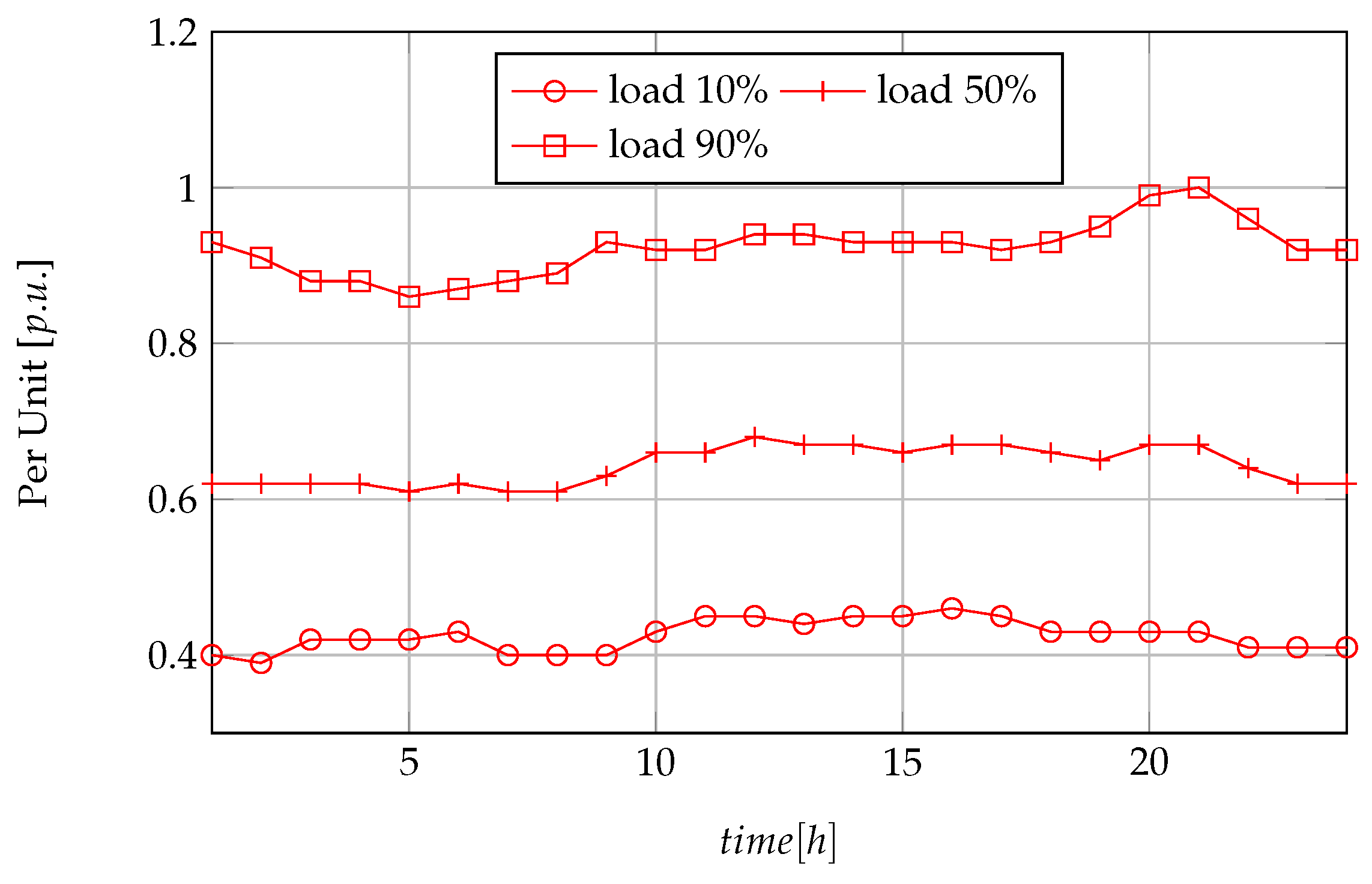
3.2. Electrical Load Forecasts

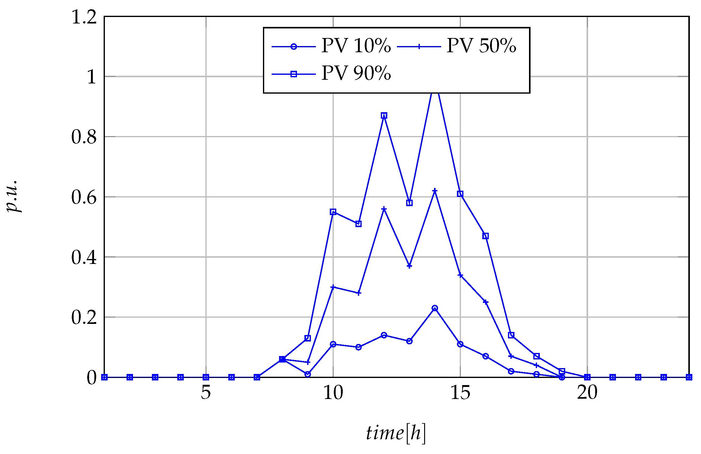
First, to form the offline dataset for the forecast, the recorded hourly electrical consumption from the smart meters located in a rural neighborhood in Evora, Portugal, was used. The data corresponded to 226 households; hence, 226 time series were obtained for 8760 h during the year 2015. In order to fit the parameters of the forecast model, the defined training period was the range 1 January–30 September, resulting in 6552 values. The test period corresponded to the range 1 October–31 December (2208 values).

The main input for the model was defined as: (1) the historical electrical consumption measurement; and (2) the local outside temperature. Regarding the historical demand measured with the smart meters, two values were taken into account: (a) the recorded measurement of demand for the same time period in the previous day: $D_{t-24}$, which provided information related to daily seasonality; and (b) the median of the measured data during the previous week: ${\overline{D}}_t=median(D_{t-24},\dots ,D_{t-168})$, to capture recent behavior. Regarding local outside temperature, a Numerical Weather Prediction Model (NWP) coming from the European Centre for Medium-Range Weather Forecasts (ECMWF) was used to feed the model with the predictions made on the previous day (${\widehat{T}}_t$).

The day-ahead probabilistic forecast was based on an additive model, which produced for each time-frame t quantile levels of hourly-forecasted electrical load. Three independent inputs, i.e., the measured demand 24 h before the forecast time-frame, the median of the demand during the previous week, and the outside temperature forecast, were used to obtain three smoothing spline functions ($\alpha$, $\beta$, $\gamma$), which were fitted to the data belonging to the training period and excluding data of the test period. A fit was carried out for each time-frame to obtain the quantile-demand forecast (${\widehat{D}}_t^{\tau }$) at levels $\tau =0.1,0.2,\dots 0.9$:

$${\widehat{D}}_t^{\tau }={\alpha }_h^{\tau }({\widehat{T}}_t)+{\beta }_h^{\tau }(D_{t-24})+{\gamma }_h^{\tau }({\overline{D}}_t)$$

(51)

To test the performance of the additive model, two scores were used: i.e., (1) reliability between two successive quantile levels; and (2) the Normalized Quantile Score (NQS). More details of the forecast model, the input data, and the performance can be found in [36].

3.3. PV Forecasts

The model proposed to obtain PV forecast was a conditional kernel density estimator of the power distribution based on the irradiance level forecast. A statistical model to forecast the PV production was considered by using the information from NWP of surface solar irradiance. The parameters were estimated for the corresponding time-frame in order to integrate interaction between the Sun’s trajectory, the PV panels’ orientation, and the shadow effect. It also allowed taking into account the influence of the temperature on the efficiency of the PV system. The data of surface solar irradiation came from the ECMWF, and the dataset of PV production came from the smart meter roll-out. Offline data corresponded one year of readings from 20 April 2014–20 April 2015.

To assess the performance of the probability forecasts, two criteria were used: reliability and sharpness. Reliability in this case was used to measure the percentage of observations that exceeded a certain quantile forecast during the evaluation period, with respect to the total number of observations. Sharpness measures the degree of concentration of the distribution, which was expected to be low for good forecast models.

The obtained probabilistic forecasts were associated with quantiles $10\%,20\%,\dots ,90\%$, similar to the ones obtained for electrical load forecast. For more details on the PV forecast method, the work in [37] is suggested as complementary reading.

An example of the forecasts of electrical load and PV used in this paper is shown in Figure 4 and Figure 5.

3.4. Thermal Load Forecasts

To model users’ thermal consumption, a normalized thermal load pattern was taken from [27] and scaled with the total forecast demand in each household. This was done given the absence of data for thermal load in the real-life demonstrator. An example of the obtained synthetic data is shown in Figure 6. These data can also be interpreted as the thermal comfort interval of each household. This information is especially useful for defining comfort confidence intervals in robust optimization formulations, as shown in Section 3.

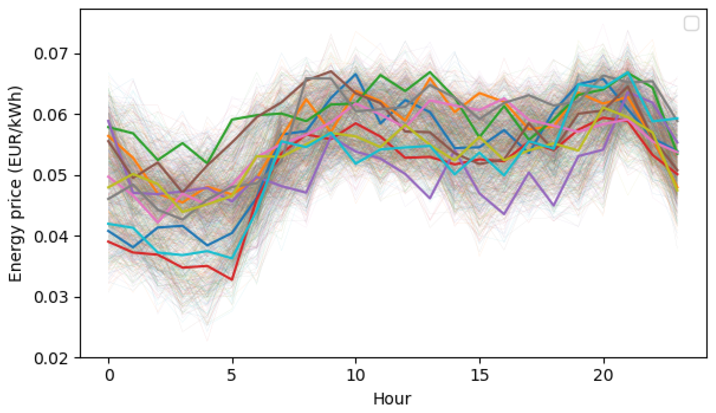
3.5. Energy Price Forecasts

The ENTSOEdatabase [38] was used to source hourly electricity prices, and the data were formed by the last three months prior to the day of dispatch. For a particular simulation, the prices for the same weekday over the three previous months were used to train the model and obtain a price forecast trajectory. The dataset belonged to the Portuguese market and for the period comprising August 2015–November 2015. The period of time was selected to have available input for 90 days and to match the period of price forecasts with the available PV and load forecasts (November 2015) to have a coherent set of data for simulations.

The Python package “scikit-learn” [39] was used to train a KDE model. The KDE was used to obtain percentiles 10% and 90%, which served to create the uncertainty intervals for the ARO. The estimation can also be used to create scenarios that are afterwards fed into the reduction technique and then used in stochastic optimization as explained at the beginning of Section 3.1.

The motivation for using this approach to create price forecasts was three-fold:

• We wanted to avoid over-simplified calculations of the uncertainty set for the robust optimization models, such as arbitrary deviations from the mean or expected forecasted values, which is a common practice in the literature [9,15,30,40] for creating confidence intervals when using robust optimization approaches.
• The dataset of 90 days was used to capture the seasonality of price-trajectories. In addition, given the obvious higher presence of weekdays in the dataset, the decision of using the same weekday to create the forecasts and not the complete 90-day data as input responded to: (a) avoiding price trajectories that mimic weekday behavior when the analysis is performed on a weekend day; or (b) avoiding the presence of the low price values that typically result during weekends, when analyzing weekdays.
• Although the focus of this paper is not on advanced forecast techniques, our approach allows creating the confidence interval with realistic information that is suitable for the practical optimization problem. This way, we avoid the heavy burden on complex forecast tools and detailed probabilistic information, which is one of the advantages of using robust optimization, as explained in Section 1.

3.6. Performance Evaluation

Performance aims to evaluate the ability of the aggregator to comply with the committed day-ahead energy while minimizing the total operation cost when faced with multiple sources of uncertainty. Monte Carlo simulation was used to test the robustness of the proposed approach for several patterns of random generated prices, consumption, and PV production during the operation day. The total cost calculation when these random values were generated and used as input was given by the day-ahead energy payments, the equivalent cycling cost of the batteries, and the penalization due to imbalances produced by real-time production/consumption in each household. The Monte Carlo simulation returned a measure of the performance in terms of average cost and Standard Deviation (SD), as a measure of the risk related to a particular robust bidding strategy. Each particular strategy was formed by a set of values of the budget of uncertainty $\Gamma$ and used as the input for a robust optimization problem, which in turn returned a set of values of the energy committed in the day-ahead energy market.

The outline of the performance methodology is presented in Figure 7. The number of simulations (stop criteria) was limited to the maximum between (a) 1000 trials and (b) the number of trials to achieve a margin of error of a maximum of 1% with a confidence interval of 95%.

The cost of each trial is given in the following expression:

$$C^{trial}=C^{ws}+C^{cyc}$$

(52)

where $C^{ws}$ is the result of solving the following optimization problem:

$$\begin{array}{cc} & \mathrm{minimize}{C}^{ws}=(26)\end{array}$$

(53)

$$\begin{array}{cc}\hfill \mathrm{s}.\mathrm{t}.& \\ & \mathrm{constraints}:(2)–(14)\end{array}$$

(54)

Given that each trial corresponded to a deterministic optimization problem, cycling Constraints (17)–(25) were included in the model, but the equivalent degradation cost ($C^{cyc}$) was calculated after the optimization process with the last term of Equation (26). This helps to reduce computational time while taking the equivalent degradation costs into account in the performance evaluation.

4. Simulations and Results

4.1. Input Data

The 25 households in the aggregation were located in an LV-rural network in Evora, Portugal. In total, there were 25 PV panels, 16 batteries, and 15 EWHs.

Fifteen batteries were rated 3 kW/3.3 kWh, and one was rated 10 kW/20 kWh. PV panels were rated 1.5 kWp. The cycling behavior of BESS was taken from the technical sheet in [41], and the initial cost was 500 €/kWh [42]. The rated power/energy for the EWHs was 1.5 kW/3 kWh according to the information available from the real-life demonstrator and typical values from technical specifications, and thermal resistance/capacitance was 568 (°C/kW)/0.3483 (kWh/°C), in line with [24]. Python was used as the programming language to set up the simulations and solve the optimization problems.

4.2. Simulation Setup

The input for each optimization was composed of the information of the devices, the forecasts, and the uncertainty budget $\Gamma :\{{\Gamma }^{DA},{\Gamma }^{D/PV},{\Gamma }^{th}\}$. For unified ARO schemes, ${\Gamma }^D$ was used, and ${\Gamma }^{PV}$ was used for separated approaches. The outcome of each uncertainty budget analyzed was an energy schedule to be purchased or sold in the wholesale market $P^E$. This solution was then tested with the performance scheme described in Section 3.6 such that an average cost and an SD deviation were obtained. These two results describe the performance of each robust solution.

There were four main robust optimization problems according to the alternatives defined in Section 3, which corresponded to solving the following problems:

• Unified Complete ARO (UCARO):

  $$\begin{array}{c}\mathrm{minimize}(27)\end{array}$$

  (55)

  $$\begin{array}{cc}\hfill \mathrm{s}.\mathrm{t}.& \\ & \mathrm{constraints}:(5)–(10),(12)–(14),(17)–(25),(28)–(37),(39)–(41)\end{array}$$

  (56)

  which corresponds to the robust counterpart when all sources of uncertainty are treated with ARO and PV and demand uncertainty are compacted in the form of net load. The resulting single parameter ${\Gamma }^D$ was employed to model these two sources of uncertainty.
• Separated Complete ARO (SCARO):

  $$\begin{array}{c}\mathrm{minimize}(27)\end{array}$$

  (57)

  $$\begin{array}{cc}\hfill \mathrm{s}.\mathrm{t}.& \\ & \mathrm{constraints}:(5)–(10),(12)–(14),(17)–(25),(28)–(34),(46)–(50),(39)–(41)\end{array}$$

  (58)

  which is the robust counterpart when all sources of uncertainty are treated with ARO and PV and demand uncertainty are treated in separate forms, resulting in two different uncertainty budgets, i.e., ${\Gamma }^{PV}$ and ${\Gamma }^D$. In this case, it was assumed that ${\Gamma }^{th}={\Gamma }^D$, to reflect equal uncertainty budget values for both electrical and thermal demand.
• Unified Hybrid Stochastic Robust Optimization (UHSRO):

  $$\begin{array}{c}\mathrm{minimize}(44)\end{array}$$

  (59)

  $$\begin{array}{cc}\hfill \mathrm{s}.\mathrm{t}.& \\ & \mathrm{constraints}:(5)–(10),(12)–(14),(17)–(25),(35)–(37),(39)–(41)\end{array}$$

  (60)
  This problem corresponds to the robust counterpart when stochastic optimization is used to model price uncertainty and ARO is used to model thermal consumption, PV, and electrical demand uncertainty, with the latter two treated in a unified form.
• Separated Hybrid Stochastic Robust Optimization (SHSRO):

  $$\begin{array}{c}\mathrm{minimize}(44)\end{array}$$

  (61)

  $$\begin{array}{cc}\hfill \mathrm{s}.\mathrm{t}.& \\ & \mathrm{constraints}:(5)–(10),(12)–(14),(17)–(25),(46)–(50),(39)–(41)\end{array}$$

  (62)
  This is the robust counterpart when stochastic optimization is used to model price uncertainty and ARO is used to model thermal consumption, PV, and electrical demand uncertainty, with the latter two treated in a separate form.

Comparisons were performed as a result of considering several combinations of aspects according to the different formulations, i.e., complete ARO versus hybrid stochastic/robust approaches, traditional $\Gamma$ versus ${\Gamma }^2$, and unified robust parameter versus separated PV-load robust parameter. All of the combinations resulted in eight alternatives to be evaluated, which are detailed as follows:

• Alternative 1: UCARO scheme with traditional $\Gamma$.
• Alternative 2: SCARO scheme with traditional $\Gamma$.
• Alternative 3: UCARO scheme with ${\Gamma }^2$.
• Alternative 4: SCARO scheme with ${\Gamma }^2$.
• Alternative 5: UHSRO scheme with traditional $\Gamma$.
• Alternative 6: SHSRO scheme with traditional $\Gamma$.
• Alternative 7: UHSRO scheme with ${\Gamma }^2$.
• Alternative 8: SHSRO scheme with ${\Gamma }^2$.

The eight alternatives were evaluated with several combinations of budgets of uncertainty to calculate average cost and SD. The solutions with the best trade-off between cost and SD from the Pareto optimality standpoint were selected as the best solutions; hence, eight Pareto fronts can be found and depicted, each belonging to each alternative.

As stated in the Introduction, the robust formulation in [30] was a building block in this paper and corresponds more specifically to Alternative 1. However, even if the philosophy of the robust mathematical model followed the same line, direct comparison of the specific numerical results with [30] is not adequate, provided that:

• Both robust models were fed with different information, specifically for prices. In [30], the price forecasts were obtained with a persistence model and a deviation of 10% from the central value. In this paper, the KDE and quantile calculation were used to create the confidence interval. The difference in the input data regarding the uncertainty set will lead the optimization of the algorithm towards different setpoints in a different search space; hence, the direct comparison is not adequate.
• In [30], random price values for the performance evaluation were generated using a uniform distribution around a central value that came from the same persistence model. In this paper, we propose a different approach based on KDE, which will lead to a misleading comparison of average cost and SD values after Monte Carlo simulation, given the different nature of the data.

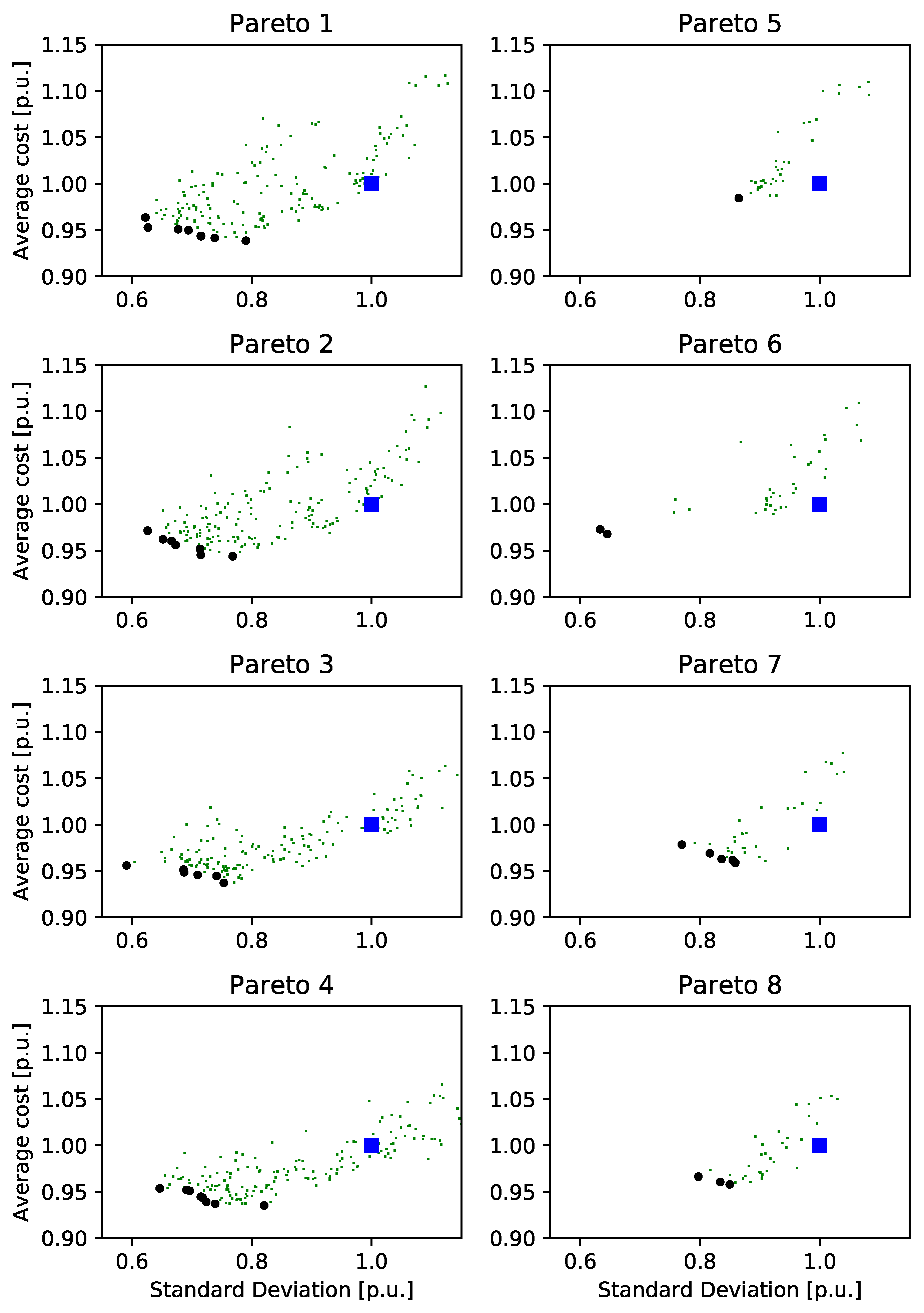
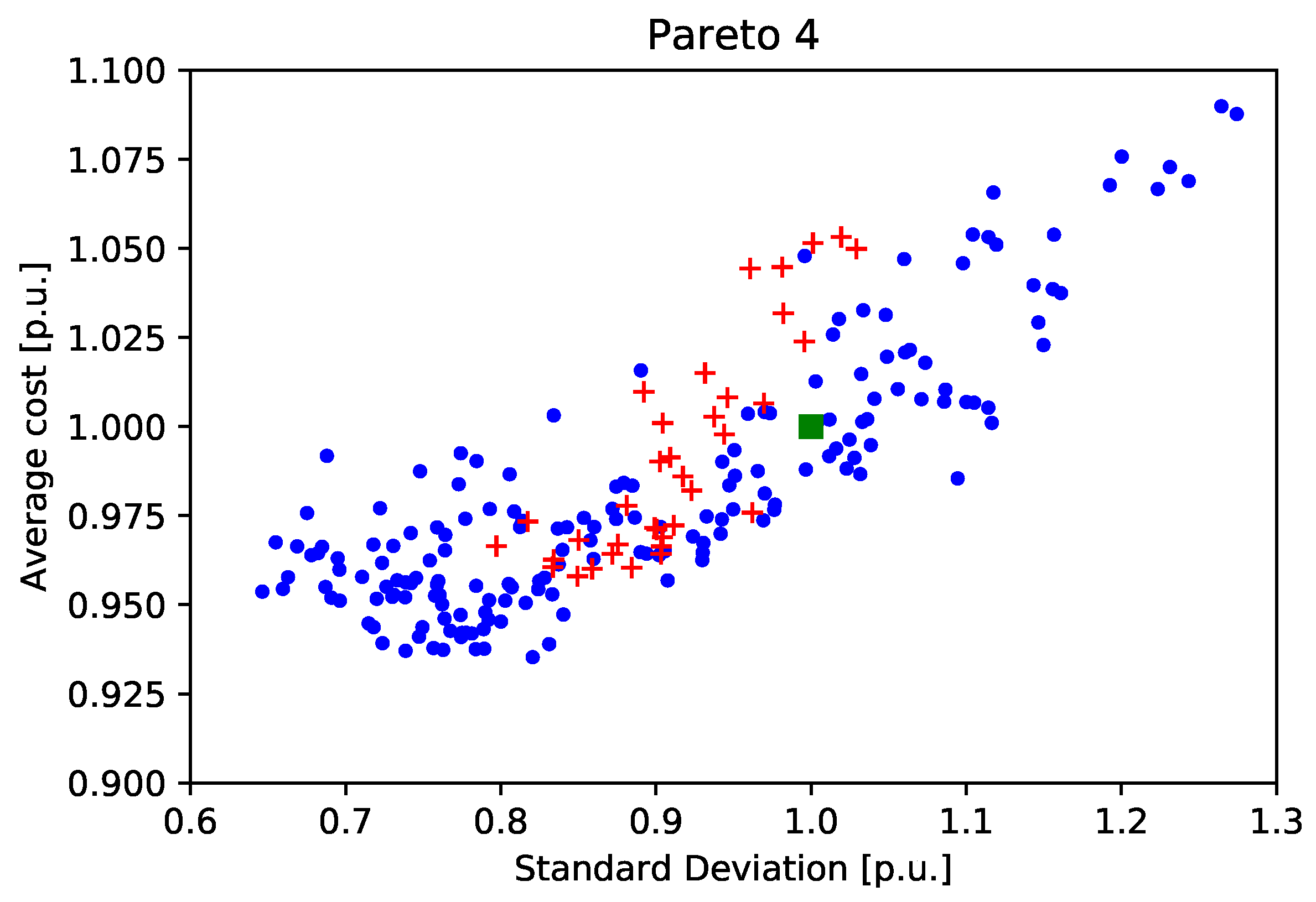
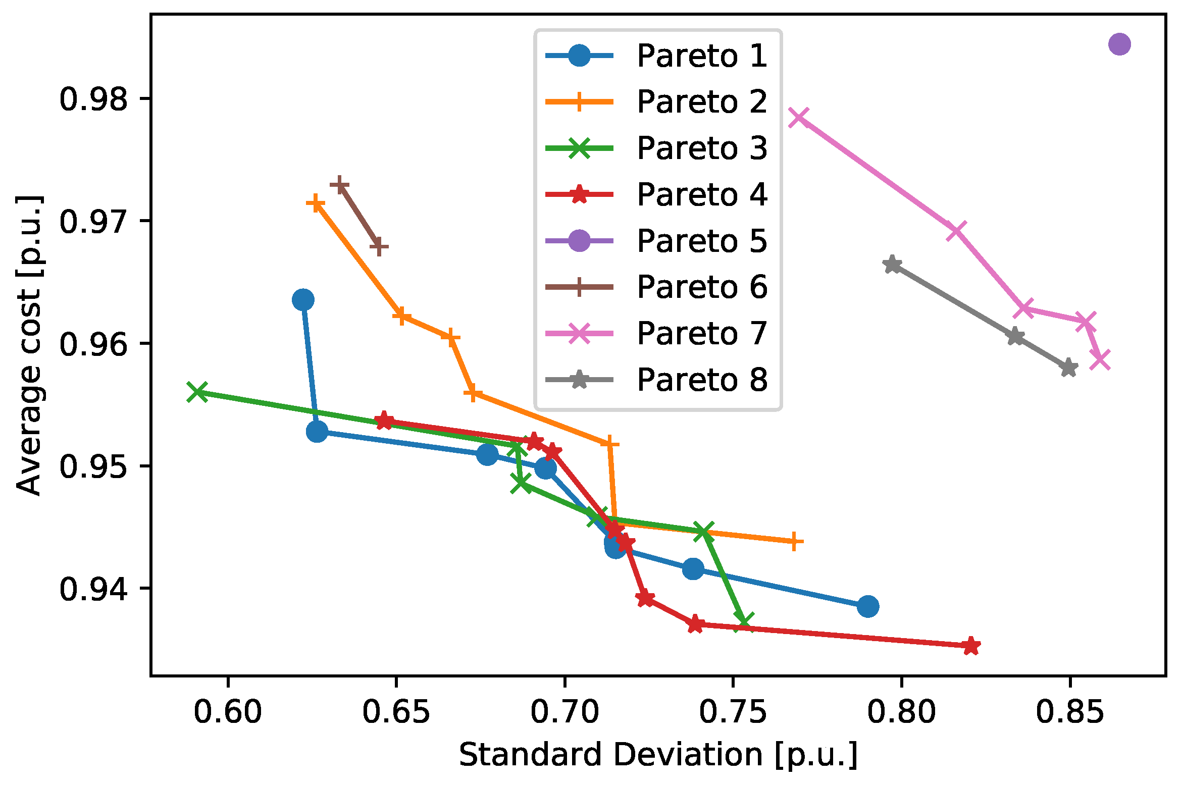
A sensitivity analysis of the impact of scenarios was carried out to analyze the behavior of the stochastic formulation. A number of samples were first created by using the KDE, and afterwards, the scenario reduction technique was used to run several stochastic optimization problems ranging from 3–50 scenarios. In this case, uncertainty in PV and demand was neglected to isolate price scenarios’ impact and visualize stabilization of the solution. The solution for 50 scenarios was taken as the base value to calculate the error of each stochastic problem. The result is shown in Figure 8.

The error showed a decreasing behavior as the number of scenarios increased. For the simulations run, the range of 10–20 scenarios ensured, for the most part, errors below 0.5%. In the case of the present paper, we used 12 scenarios to solve the hybrid stochastic/robust formulations (Alternatives 5–8). With this selection, low values of error were achieved while avoiding an increase in the problem size and the consequent increase in computational effort.

4.3. Simulations

The performance of the alternatives was calculated based on the algorithm presented in Section 3.6. To define the uncertainty budgets to be evaluated, a step of six was defined for ${\Gamma }^{DA}$, resulting in the following values: 0, 6, 12, 18, and 24, provided that cardinality was 24, i.e., the maximum number of parameters that can deviate from central values. For the remaining $\Gamma$s, a step of 0.2 was used, resulting in the set of values: 0, 0.2, 0.4, 0.6, 0.8, and 1. All of these values were combined in order to map and analyze different levels of robustness and to determine which combinations were the best from the cost and SD standpoint. For complete ARO schemes (Alternatives 1–4), there were $5\times 6\times 6=180$ possible combinations of budgets. For the hybrid, there were $6\times 6=36$ combinations provided that there was no uncertainty budget for prices.

Figure 9 shows the eight Pareto fronts (black dots •) for the proposed alternatives. The green dots (•) represent dominated solutions (from the Pareto-optimality perspective) associated with different combinations’ uncertainty budget, but that, in all cases, turned out to be less attractive from the cost or SD point of view. The deterministic solution is depicted as a blue square (■).

In all cases, solutions always exist that result in more attractive cost and SD at the time, compared to the deterministic solution. This means that certain combinations of ${\Gamma }^{DA}$, ${\Gamma }^{D/PV}$, and ${\Gamma }^{th}$ exist that outperform deterministic and some other conservative robust solutions. These solutions are of particular interest to define an appropriate day-ahead energy commitment plan in the wholesale market, as they can guarantee lower operational cost and risk when facing uncertainty during real-time operation. The selection of a particular solution, corresponding to a particular uncertainty budget, will depend on the aggregator and its strategy to prioritize expected cost or decrease risk. In general, complete robust approaches (Alternatives 1–4) present lower associated costs than hybrid schemes (Alternatives 5–8). In addition, Pareto fronts were formed, in general, by a higher number of points, also for Alternatives 1–4.

Table 1. Details of the Pareto front values and improvements with respect to the deterministic solution. * ${\Gamma }^D$ is valid for the unified approach, and ${\Gamma }^{PV}$ is valid for the separated approach.

Pareto Front	${\mathbf{\Gamma }}^{\mathit{DA}}$/${\mathbf{\Gamma }}^{\mathit{D}/\mathit{PV}}$ */${\mathbf{\Gamma }}^{\mathit{th}}$	Cost (p.u.)	SD (p.u.)
Pareto 1	${\Gamma }_1^1$: 12/0/0.6	0.941	0.738
	${\Gamma }_2^1$: 12/0.2/0.2	0.938	0.790
	${\Gamma }_3^1$: 12/0.2/0.8	0.949	0.694
	${\Gamma }_4^1$: 12/0.2/1	0.950	0.677
	${\Gamma }_5^1$: 12/0.4/0	0.943	0.714
	${\Gamma }_6^1$: 12/0.4/0.6	0.943	0.715
	${\Gamma }_7^1$: 12/0.4/0.8	0.952	0.626
	${\Gamma }_8^1$: 12/0.6/0.6	0.964	0.622
Pareto 2	${\Gamma }_1^2$: 12/0/0.4	0.952	0.713
	${\Gamma }_2^2$: 12/0/0.6	0.962	0.651
	${\Gamma }_3^2$: 12/0.2/0.2	0.944	0.768
	${\Gamma }_4^2$: 12/0.2/0.4	0.945	0.715
	${\Gamma }_5^2$: 12/0.4/0.6	0.972	0.626
	${\Gamma }_6^2$: 12/0.6/0	0.956	0.673
	${\Gamma }_7^2$: 12/0.8/0.2	0.961	0.666
Pareto 3	${\Gamma }_1^3$: 12/0/0.4	0.937	0.753
	${\Gamma }_2^3$: 12/0/1	0.956	0.591
	${\Gamma }_3^3$: 12/0.2/0	0.945	0.741
	${\Gamma }_4^3$: 12/0.2/0.2	0.949	0.710
	${\Gamma }_5^3$: 12/0.2/0.6	0.949	0.687
	${\Gamma }_6^3$: 12/0.2/1	0.952	0.686
Pareto 4	${\Gamma }_1^4$: 12/0/0	0.945	0.715
	${\Gamma }_2^4$: 12/0.2/0.2	0.937	0.739
	${\Gamma }_3^4$: 12/0.8/0	0.951	0.696
	${\Gamma }_4^4$: 18/0/0.2	0.943	0.718
	${\Gamma }_5^4$: 18/0/0.4	0.952	0.691
	${\Gamma }_6^4$: 18/0.2/0.4	0.954	0.646
	${\Gamma }_7^4$: 18/0.6/0	0.939	0.724
	${\Gamma }_8^4$: 18/0.6/0.2	0.935	0.821
Pareto 5	${\Gamma }_1^5$: Stochastic/0.2/0.2	0.984	0.864
Pareto 6	${\Gamma }_1^6$: Stochastic/0.0/0.4	0.968	0.645
	${\Gamma }_2^6$: Stochastic/0.2/0	0.973	0.633
Pareto 7	${\Gamma }_1^7$: Stochastic/0.0/0.8	0.959	0.859
	${\Gamma }_2^7$: Stochastic/0.2/0	0.963	0.836
	${\Gamma }_3^7$: Stochastic/0.2/0.4	0.969	0.816
	${\Gamma }_4^7$: Stochastic/0.2/0.6	0.962	0.855
	${\Gamma }_5^7$: Stochastic/0.4/0.2	0.978	0.769
Pareto 8	${\Gamma }_1^8$: Stochastic/0.0/0.2	0.958	0.850
	${\Gamma }_2^8$: Stochastic/0.2/0	0.966	0.797
	${\Gamma }_3^8$: Stochastic/0.4/0	0.961	0.834

shows the values of $\Gamma$ that led to the points of each Pareto. Each of the $\Gamma$ configurations present in the Pareto front can be read in the following form: ${\Gamma }_m^n$ represents the $m^{\mathrm{th}}$ point in the $n^{\mathrm{th}}$ Pareto front, or in alternative n. For instance, for Pareto Front 1 in Table 1, there were eight points, denoted by Super-index 1. The points in this Pareto front were the best obtained with the complete robust approach (UCARO, Alternative 1).

When inspecting each of the found Pareto fronts, it can be seen that complete ARO formulations (Alternatives 1–4) outperformed HSR approaches (Alternatives 5–8). The best obtained solution from the perspective of average cost was ${\Gamma }_8^4$, which belongs to Alternative 4: SCARO formulation with ${\Gamma }^2$. This solution improved the cost performance of the deterministic solution by 6.5%. The best obtained solution from the perspective of SD was ${\Gamma }_2^3$, which belongs to Alternative 3: UCARO formulation with ${\Gamma }^2$. This solution improved the SD of the deterministic solution by 40.9%.

It was also found that the number of iterations in the Monte Carlo simulation to achieve performance convergence was related to the chosen alternative for $\Gamma$. For instance, the number of Monte Carlo iterations before convergence for each of the Alternatives 1–8 was respectively: 766, 762, 389, 394, 920, 872, 403, 402. By inspecting this result, the lower number of iterations was associated with Alternatives 3, 4, 7, and 8, which are those related to ${\Gamma }^2$.

Other descriptors used to assess the performance of each individual alternative are shown in

Table 2. Descriptors and assessment of each alternative. * Number of points/participation of each alternative in the global merged Pareto.

Alt.	Av. Cost All Points	Av. Cost Pareto	Median Cost All Points	Av. SD All Points	Av. SD Pareto	Median SD All Points	Global Pareto *	Best Cost?	Best SD?
1	0.994	0.948	0.985	0.8355	0.697	0.817	4	No	No
2	0.995	0.956	0.985	0.8426	0.688	0.810	0	No	No
3	0.986	0.947	0.976	0.870	0.695	0.834	3	No	Yes
4	0.982	0.945	0.972	0.890	0.719	0.855	4	Yes	No
5	1.029	0.984	1.012	0.946	0.865	0.928	0	No	No
6	1.025	0.970	1.012	0.925	0.639	0.934	0	No	No
7	0.997	0.966	0.980	0.902	0.827	0.874	0	No	No
8	0.991	0.962	0.979	0.913	0.827	0.904	0	No	No

. In this case, there were nine descriptors based on the results shown in Figure 9, which are described as follows:

• Average cost of all points: average value of the y-axis points belonging to each alternative.
• Average cost of Pareto points: average value of the y-axis Pareto points belonging to each alternative.
• Median cost of all points: median of the y-axis points belonging to each alternative.
• Average SD of all points: average value of the x-axis points belonging to each alternative.
• Average SD of Pareto points: average value of the x-axis Pareto points belonging to each alternative.
• Median SD of all points: median of the x-axis points belonging to each alternative.
• Number of points in the global Pareto: when all points of the performance of each alternative are combined, the number of points present in the global Pareto from each alternative.
• Best cost: identifies if the alternative was able to find the best global cost.
• Best SD: identifies if the alternative was able to find the best global SD.

Table 2 shows the results of the descriptors calculated for each individual alternative. The results show that Alternative 4 tended to perform better than the rest for the cost-related descriptors. In addition, this alternative presented four points in the final global Pareto front after combining all of the alternatives. Moreover, only one descriptor associated with hybrid approaches performed better, which was the case for Alternative 6.

When we analyzed the results in Table 2 from the perspective of the proposed modifications to the model, i.e., complete ARO or hybrid ARO, separated or unified budget, $\Gamma$ or ${\Gamma }^2$, the following results were obtained. Complete ARO schemes were present in 8/9 of the best-ranked descriptors’ values. In addition, separate alternatives were present in 7/9 of the best values obtained for the descriptors. Finally, ${\Gamma }^2$ modifications participated in 6/9 best values. Additionally, as mentioned before, better convergence capabilities in the performance evaluation were shown by option ${\Gamma }^2$. The results demonstrate the clear advantage of using complete ARO schemes versus hybrid, showing that separate formulations performed better than unified approaches and that ${\Gamma }^2$ outperformed $\Gamma$. These three performing features identified were all present together in Alternative 4, which is in fact the most interesting alternative from the perspective of cost-related descriptors.

If the information contained in Pareto 4 and 8 are analyzed, the different solutions obtained for Alternatives 4 and 8 can be detailed. Figure 10 shows this information. It can be seen that the dominant points from the standpoint of average cost and SD were associated with the ARO formulation (blue dots). Although some solutions for the HSR approach (red crosses) outperformed the deterministic solution and some ARO solutions, Alternative 4 always featured better solutions.

Figure 11 shows the eight obtained Pareto fronts combined in the same axis. This figure allows us to visualize the descriptor “Global Pareto”, which helps to determine the best global solutions from the cost and SD standpoints. For instance, the best trade-off set of solutions was formed by 11 points, four belonging to Alternative 1 (blue circles), three to Alternative 3 (green X), and four to Alternative 4 (red stars). These 11 solutions contained the best combinations of both measured quantities after the performance evaluation. The remaining points represent dominated solutions, i.e., one can always find at least one point among the 11 trade-off solutions that is better in both objectives at the same time. It can also be visualized that hybrid solutions (Alternatives 5–8) are less attractive when compared to robust approaches.

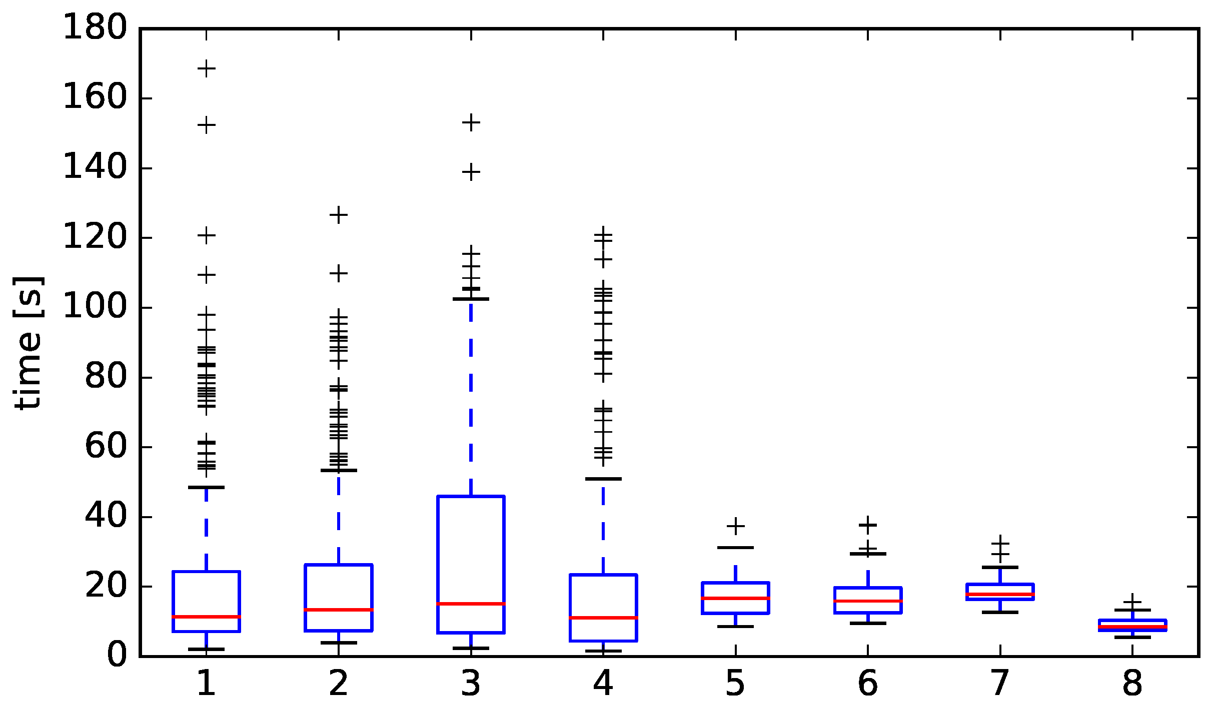
4.4. Some Remarks about Computational Times

Figure 12 presents the boxplots of computational times for the eight alternatives presented in the previous subsection. In general, Alternatives 1–4 presented higher dispersion of data in several cases with computational times ranging from 1–3 min. These solutions are related to the combinations of robust parameters mainly for ${\Gamma }^{DA}$ different from zero. Hybrid stochastic/robust (Alternatives 5–8) solutions had more consistent computational times even if the median was in some cases higher than those obtained for complete ARO cases (Alternatives 1–4). Due to the combinations of control parameters, 180 robust optimization problems had to be solved for Alternatives 1–4, and 36 hybrid problems had to be solved for Alternatives 5–8, leading to more intensive overall times for complete robust approaches.

Table 3. Details of computational time for each alternative.

Alternative	1	2	3	4	5	6	7	8
Overall computational time (s)	4274	4323	5717	4004	631	631	686	321
Median (s)	11	13	15	11	16	15	17	8
Average (s)	23	24	31	22	17	17	19	9

shows a summary of different obtained values for each alternative.

Higher overall times for Alternatives 1–4 are explained by the fact that more individual optimization problems had to be solved to cope with the combinations of budgets of uncertainty. Moreover, lower median values were obtained for complete robust alternatives. However, average times were higher when compared to hybrid schemes. This is explained by the presence of high-value outliers for Alternatives 1–4. Although the hybrid schemes had more attractive overall computational times, the quality of the solutions obtained remained a drawback when compared to complete robust approaches, as explained in detail in the previous subsection.

5. Conclusions

When using strong duality to obtain the robust counterpart of the deterministic model, and for the specific case of PV and electrical load, an additional calculation was established to obtain net load in each time-step. This formulation allows for a more compact energy balance equation, provided that two sources of uncertainty are converted into one. This results in one unified uncertainty budget to control net load conservatism. In addition, $3\times T$ dual variables and $2\times T$ new constraints were introduced. An alternative was also explored by maintaining separate budgets and dual variables for electrical load and PV. Although this formulation resulted in a larger optimization problem, in some cases, separate handling of both sources of uncertainty impacted the performance of the solutions and had better mitigation of over-conservatism.

Alternative 1 presented in this paper was the one more directly related to the formulation in [30]. However, here, we present the advantage of expanding and exploring modified formulations in a more complete framework with multiple descriptors to assess each alternative. The general idea of the advantage of using robust models to avoid imbalances (and penalties) remains as a key finding in both works.

In general, ARO ensures a guaranteed minimum cost and lower imbalances. Depending on the market design for aggregators and imbalance prices to settle deviations, overall performance and absolute values of cost and SD decrease can vary.

The proposed performance analysis consisted of detecting the combination of robust parameters yielded in the set of Pareto-optimal solutions from the standpoint of cost and standard deviation, when the obtained solution was subject to random realizations of the uncertain variables. Hybrid stochastic/robust and complete robust alternatives were compared. For some combinations of robust parameters, the deterministic solution outperformed some HSR and complete ARO solutions. Nonetheless, HSR and complete ARO solutions can always be found in such a way that both cost and SD outperform the deterministic approach.

For the case of HSR, price scenarios were created using KDE. A backward reduction technique based on the Kantorovich distance was used to obtain a reduced set of scenarios. For the run simulations, the hybrid approach performed better than the deterministic approach and some of the ARO solutions. However, some ARO solutions performed better than the HSR from both average cost and SD standpoints.

In particular, Alternative 4, separated complete ARO with ${\Gamma }^2$, performed better than the other alternatives in several of the measured descriptors. In also presented the lowest average operational cost of all of the simulations that we ran. In this case, separate treatment of uncertainty for load and PV identified a dual equivalent (robust counterpart) and hence two separate robust parameters to adjust and achieve lower costs and SDs. In addition, this alternative led to lower Monte Carlo simulations to achieve convergence under the performance evaluation.

References

1. Carreiro, A.M.; Jorge, H.M.; Antunes, C.H. Energy management systems aggregators: A literature survey. Renew. Sustain. Energy Rev. 2017, 73, 1160–1172. [Google Scholar] [CrossRef]
2. European Commission. Proposal for a Regulation of the European Parliament and of the Council on the Internal Market for Electricity; Publications Office of the European Union: Brussels, Belgium, 2016. [Google Scholar]
3. Bessa, R.; Moreira, C.; Silva, B.; Matos, M. Handling renewable energy variability and uncertainty in power systems operation. Wiley Interdiscip. Rev. Energy Environ. 2014, 3, 156–178. [Google Scholar] [CrossRef]
4. Alizadeh, M.; Moghaddam, M.P.; Amjady, N.; Siano, P.; Sheikh-El-Eslami, M. Flexibility in future power systems with high renewable penetration: A review. Renew. Sustain. Energy Rev. 2016, 57, 1186–1193. [Google Scholar] [CrossRef]
5. Burger, S.; Chaves-Ávila, J.P.; Batlle, C.; Pérez-Arriaga, I.J. A review of the value of aggregators in electricity systems. Renew. Sustain. Energy Rev. 2017, 77, 395–405. [Google Scholar] [CrossRef]
6. Liang, H.; Zhuang, W. Stochastic Modeling and Optimization in a Microgrid: A Survey. Energies 2014, 7, 2027–2050. [Google Scholar] [CrossRef]
7. Birge, J.R.; Louveaux, F. Introduction to Stochastic Programming, 2nd ed.; Springer: New York, NY, USA, 2011. [Google Scholar]
8. Bertsimas, D.; Sim, M. Robust discrete optimization and network flows. Math. Program. Ser. B 2003, 98, 49–71. [Google Scholar] [CrossRef] [Green Version]
9. Liu, G.; Xu, Y.; Tomsovic, K. Bidding Strategy for Microgrid in Day-Ahead Market Based on Hybrid Stochastic/Robust Optimization. IEEE Trans. Smart Grid 2016, 7, 227–237. [Google Scholar] [CrossRef]
10. Wang, R.; Wang, P.; Xiao, G. A robust optimization approach for energy generation scheduling in microgrids. Energy Convers. Manag. 2015, 106, 597–607. [Google Scholar] [CrossRef]
11. Wang, J.; Zhong, H.; Tang, W.; Rajagopal, R.; Xia, Q.; Kang, C.; Wang, Y. Optimal bidding strategy for microgrids in joint energy and ancillary service markets considering flexible ramping products. Appl. Energy 2017, 205, 294–303. [Google Scholar] [CrossRef]
12. Hu, W.; Wang, P.; Gooi, H.B. Toward Optimal Energy Management of Microgrids via Robust Two-Stage Optimization. IEEE Trans. Smart Grid 2018, 9, 1161–1174. [Google Scholar] [CrossRef]
13. Liu, G.; Starke, M.; Xiao, B.; Tomsovic, K. Robust optimization-based microgrid scheduling with islanding constraints. IET Gener. Transm. Distrib. 2017, 11, 1820–1828. [Google Scholar] [CrossRef]
14. Wang, L.; Li, Q.; Ding, R.; Sun, M.; Wang, G. Integrated scheduling of energy supply and demand in microgrids under uncertainty: A robust multi-objective optimization approach. Energy 2017, 130, 1–14. [Google Scholar] [CrossRef]
15. Kuznetsova, E.; Li, Y.F.; Ruiz, C.; Zio, E. An integrated framework of agent-based modeling and robust optimization for microgrid energy management. Appl. Energy 2014, 129, 70–88. [Google Scholar] [CrossRef]
16. Gupta, R.; Gupta, N.K. A robust optimization based approach for microgrid operation in deregulated environment. Energy Convers. Manag. 2015, 93, 121–131. [Google Scholar] [CrossRef]
17. Wang, J.; Li, P.; Fang, K.; Zhou, Y. Robust Optimization for Household Load Scheduling with Uncertain Parameters. Appl. Sci. 2018, 8, 575. [Google Scholar] [CrossRef]
18. Diekerhof, M.; Peterssen, F.; Monti, A. Hierarchical Distributed Robust Optimization for Demand Response Services. IEEE Trans. Smart Grid 2018, 9, 6018–6029. [Google Scholar] [CrossRef]
19. Zhou, Y.; Wei, Z.; Sun, G.; Cheung, K.W.; Zang, H.; Chen, S. A robust optimization approach for integrated community energy system in energy and ancillary service markets. Energy 2018, 148, 1–15. [Google Scholar] [CrossRef]
20. Bertsimas, D.; Brown, D.B.; Caramanis, C. Theory and Applications of Robust Optimization. SIAM Rev. 2011, 53, 464–501. [Google Scholar] [CrossRef] [Green Version]
21. Kilkki, O.; Seilonen, I.; Zenger, K.; Vyatkin, V. Optimizing residential heating and energy storage flexibility for frequency reserves. Int. J. Electr. Power Energy Syst. 2018, 100, 540–549. [Google Scholar] [CrossRef]
22. Li, J.; Wu, Z.; Zhou, S.; Fu, H.; Zhang, X.P. Aggregator service for PV and battery energy storage systems of residential building. CSEE J. Power Energy Syst. 2015, 1, 3–11. [Google Scholar] [CrossRef]
23. Comodi, G.; Giantomassi, A.; Severini, M.; Squartini, S.; Ferracuti, F.; Fonti, A.; Nardi, D.; Morodo, M.; Polonara, F. Multi-apartment residential microgrid with electrical and thermal storage devices: Experimental analysis and simulation of energy management strategies. Appl. Energy 2015, 137, 854–866. [Google Scholar] [CrossRef]
24. Good, N.; Karangelos, E.; Navarro-Espinosa, A.; Mancarella, P. Optimization under Uncertainty of Thermal Storage-Based Flexible Demand Response with Quantification of Residential Users’ Discomfort. IEEE Trans. Smart Grid 2015, 6, 2333–2342. [Google Scholar] [CrossRef]
25. Xu, Z.; Guan, X.; Jia, Q.S.; Wu, J.; Wang, D.; Chen, S. Performance Analysis and Comparison on Energy Storage Devices for Smart Building Energy Management. IEEE Trans. Smart Grid 2012, 3, 2136–2147. [Google Scholar] [CrossRef]
26. Ouammi, A. Optimal Power Scheduling for a Cooperative Network of Smart Residential Buildings. IEEE Trans. Sustain. Energy 2016, 7, 1317–1326. [Google Scholar] [CrossRef]
27. Li, X.; Borsche, T.; Andersson, G. PV integration in Low-Voltage feeders with Demand Response. In Proceedings of the 2015 IEEE Eindhoven PowerTech, PowerTech 2015, Eindhoven, The Netherlands, 29 June–2 July 2015. [Google Scholar]
28. Xu, B.; Zhao, J.; Zheng, T.; Litvinov, E.; Kirschen, D.S. Factoring the Cycle Aging Cost of Batteries Participating in Electricity Markets. IEEE Trans. Power Syst. 2018, 33, 2248–2259. [Google Scholar] [CrossRef] [Green Version]
29. Xu, B.; Shi, Y.; Kirschen, D.S.; Zhang, B. Optimal regulation response of batteries under cycle aging mechanisms. In Proceedings of the 2017 IEEE 56th Annual Conference on Decision and Control (CDC), Melbourne, VIC, Australia, 12–15 December 2017; pp. 751–756. [Google Scholar]
30. Correa-Florez, C.A.; Michiorri, A.; Kariniotakis, G. Robust optimization for day-ahead market participation of smart home aggregators. Appl. Energy 2018, 229, 433–445. [Google Scholar] [CrossRef]
31. He, G.; Chen, Q.; Kang, C.; Pinson, P.; Xia, Q. Optimal Bidding Strategy of Battery Storage in Power Markets Considering Performance-Based Regulation and Battery Cycle Life. IEEE Trans. Smart Grid 2016, 7, 2359–2367. [Google Scholar] [CrossRef]
32. Ortega-Vazquez, M.A. Optimal scheduling of electric vehicle charging and vehicle-to-grid services at household level including battery degradation and price uncertainty. IET Gener. Transm. Distrib. 2014, 8, 1007–1016. [Google Scholar] [CrossRef]
33. Duggal, I.; Venkatesh, B. Short-Term Scheduling of Thermal Generators and Battery Storage With Depth of Discharge-Based Cost Model. IEEE Trans. Power Syst. 2015, 30, 2110–2118. [Google Scholar] [CrossRef]
34. Bertsimas, D.; Sim, M. The Price of Robustness. Oper. Res. 2004, 52, 35–53. [Google Scholar] [CrossRef]
35. Razali, N.M.M.; Hashim, A.H. Backward reduction application for minimizing wind power scenarios in stochastic programming. In Proceedings of the 2010 4th International Power Engineering and Optimization Conference (PEOCO), Shah Alam, Malaysia, 23–24 June 2010; pp. 430–434. [Google Scholar]
36. Gerossier, A.; Girard, R.; Bocquet, A.; Kariniotakis, G. Robust Day-Ahead Forecasting of Household Electricity Demand and Operational Challenges. Energies 2018, 11, 3503. [Google Scholar] [CrossRef]
37. Bocquet, A.; Michiorri, A.; Bossavy, A.; Girard, R.; Kariniotakis, G. Assessment of probabilistic PV production forecasts performance in an operational context. In Proceedings of the 6th Solar Integration Workshop—International Workshop on Integration of Solar Power into Power Systems, Vienna, Austria, 14–15 November 2016. [Google Scholar]
38. ENTSOE Transparency. Central Collection and Publication of Electricity Generation, Transportation and Consumption Data and Information for the Pan-European Market, Day-Ahead Prices. Available online: https://transparency.entsoe.eu/transmission-domain/r2/dayAheadPrices/show (accessed on 25 January 2018).
39. Pedregosa, F.; Varoquaux, G.; Gramfort, A.; Michel, V.; Thirion, B.; Grisel, O.; Blondel, M.; Prettenhofer, P.; Weiss, R.; Dubourg, V.; et al. Scikit-learn: Machine Learning in Python. J. Mach. Learn. Res. 2011, 12, 2825–2830. [Google Scholar]
40. Ampatzis, M.; Nguyen, P.H.; Kamphuis, I.G.; van Zwam, A. Robust optimization for deciding on real-time flexibility of storage-integrated photovoltaic units controlled by intelligent software agents. IET Renew. Power Gener. 2017, 11, 1527–1533. [Google Scholar] [CrossRef]
41. SAFT Batteries Lithium Ion Battery Life. May 2014. Available online: saftbatteries.com/force_download/li_ion_battery_life__TechnicalSheet_en_0514 _Protected.pdf (accessed on 20 April 2017).
42. IRENA International Renewable Energy Agency. Battery Storage for Renewables: Market Status and Technology Outlook; International Renewable Energy Agency: Abu Dhabi, UAE, 2015. [Google Scholar]
Figure 1. Schematic diagram of the proposed aggregation of resources.
Energies 12 01019 g001
Figure 2. Fitted curve for a real-life Li-ion battery.
Energies 12 01019 g002
Figure 3. Example of Kernel Density Estimation (KDE) sampling and scenarios obtained after the backward reduction technique for energy prices.
Energies 12 01019 g003
Figure 4. Example of normalized electrical load probabilistic forecasts.
Energies 12 01019 g004
Figure 5. Example of normalized PV probabilistic forecasts.
Energies 12 01019 g005
Figure 6. Example of normalized thermal load probabilistic forecasts.
Energies 12 01019 g006
Figure 7. Performance evaluation procedure for predefined values of robust parameters Γ D A , Γ D / P V , Γ t h . * Γ D is valid for the unified approach, and Γ P V is valid for the separated approach.
Energies 12 01019 g007
Figure 8. Error evolution as a function of price scenarios for the stochastic solution for three independent trials.
Energies 12 01019 g008
Figure 9. Performance points (green dots) and Pareto fronts (•) for each Alternative 1–8. Deterministic solution in blue squares.
Energies 12 01019 g009
Figure 10. Performance points for alternative 4 (blue dots) and Alternative 8 (red crosses). Deterministic solution in green square.
Energies 12 01019 g010
Figure 11. Comparison of all Pareto points.
Energies 12 01019 g011
Figure 12. Computational time boxplots for each optimization alternative. Each datum corresponds to the optimization time for a given combination of control parameters.
Energies 12 01019 g012