Developing and Comparing Different Strategies for Combining Probabilistic Photovoltaic Power Forecasts in an Ensemble Method

Abstract

Accurate probabilistic forecasts of renewable generation are drivers for operational and management excellence in modern power systems and for the sustainable integration of green energy. The combination of forecasts provided by different individual models may allow increasing the accuracy of predictions; however, in contrast to point forecast combination, for which the simple weighted averaging is often a plausible solution, combining probabilistic forecasts is a much more challenging task. This paper aims at developing a new ensemble method for photovoltaic (PV) power forecasting, which combines the outcomes of three underlying probabilistic models (quantile k-nearest neighbors, quantile regression forests, and quantile regression) through a weighted quantile combination. Due to the challenges in combining probabilistic forecasts, the paper presents different combination strategies; the competing strategies are based on unconstrained, constrained, and regularized optimization problems for estimating the weights. The competing strategies are compared to individual forecasts and to several benchmarks, using the data published during the Global Energy Forecasting Competition 2014. Numerical experiments were run in MATLAB and R environments; the results suggest that unconstrained and Least Absolute Shrinkage and Selection Operator (LASSO)-regularized strategies exhibit the best performances for the datasets under study, outperforming the best competitors by 2.5 to 9% of the Pinball Score.

1. Introduction

Load demand and non-controllable generation powers are the main sources of uncertainty in modern electrical grids and forecasting of these issues is of the greatest interest during planning and operation stages. In particular, disposing of accurate load and generation predictions is mandatory in order to tackle and solve a large variety of power system tasks, such as market bidding, energy dispatch in smart grids and microgrids, replacement reserve scheduling, virtual power plant aggregation, and sizing of battery energy storage systems [1,2,3,4,5,6,7].

Relevant literature on load and generation forecasting is quite heterogeneous; this is highlighted by the comparative dissertations in reviews and surveys [8,9], clearly showing that no method outperforms the others in every aspect. Major efforts have been devoted to point prediction, for which researchers and practitioners often individuate Artificial Neural Networks (ANN) [10,11], K-Nearest Neighbors (KNN) [12], support vector regression [13], Random Forests (RF) [14], and multiple linear regression models [15] as the best solutions.

Historically, research efforts have often been dedicated to load forecasting, since the generation has been mainly constituted by dispatchable fossil-fueled and hydroelectric plants. Today, instead, the widespread penetration of renewable generation, and in particular of photovoltaic (PV) and wind systems, makes forecasting renewable generation essential to cope with the new power system tasks, addressing the uncertainty of the energy source. Moreover, due to the intrinsic randomness of the physical phenomenon, probabilistic PV power forecasting is more adequate to deal with the management and operation of electrical networks under uncertainties [16,17]; however, only a minor part of the existing literature has dealt with PV power forecasting under a probabilistic framework. Relevant existing approaches are based on Quantile K-Nearest Neighbors (QKNN) [18], Quantile Regression Forests (QRFs) [19], Quantile Regression (QR) [20,21], and Gradient Boosting Regression Trees [18]; these models proved their effectiveness also in recent energy forecasting competitions [16,22], since the forecasting systems developed by the highest-ranking teams were based on these nonparametric probabilistic models.

New trends in probabilistic PV power forecasting individuate the probabilistic combination of individual forecasts as a suitable solution, in order to improve the accuracy of the results [9,20,23]. Probabilistic forecast combination is not as straightforward as it seems to be at first inspection. In contrast to combining point forecasts, for which the simple weighted averaging is often a plausible solution, combining probabilistic forecasts is a much more challenging task; the combined probabilistic forecasts indeed must retain adequate properties in terms of reliability and sharpness [20,24], and the main features of a probabilistic forecast (e.g., the ascending order of predictive quantiles) must be retained also by the combined forecasts [23].

Relevant literature has addressed these aspects under different points of view [9]. Individual probabilistic forecasts can be indeed merged: (i) by a combination of the predictive cumulative distribution functions [20]; or (ii) by a combination of the predictive quantiles [23]. The first combination type has already been applied to PV power forecasting, whereas the second combination type has yet to be applied to PV power forecasting (it has been presented in [23] only for load forecasting). Nevertheless, within these two types of approach, several strategies and architectures can be developed to combine forecasts, so there is room for further investigation and improvement.

In this context, this paper aims to provide a further contribution on the probabilistic combination of PV power forecasts. The paper develops and compares different forecast combination strategies applied to three individual probabilistic models (QKNN [18], QRF [19], and QR [20,21]), which are selected among the state-of-the-art nonparametric solutions for probabilistic forecasting. The outcomes of these models are properly combined under a competitive ensemble framework, based on a weighted combination of predictive quantiles.

Estimating the combination weights is a challenging task; several estimation strategies and architectures are therefore analyzed in this paper, in order to check the effectiveness of the model combination from different perspectives, and to allow picking the best solution for combining forecasts. In particular, the competing strategies are based on unconstrained, constrained, and regularized optimization problems for estimating the weights used to combine the predictive quantiles.

To guarantee the reproducibility of the experiments, the data published in the framework of the Global Energy Forecasting Competition 2014 (GEFCOM2014) [16] are used in this paper. In order to validate the proposal, the results are compared to relevant probabilistic benchmarks in actual scenarios.

Eventually, the main contributions of this paper are:

• the development of a new competitive ensemble method that combines the outcomes of three probabilistic models, selected among the ones which have proved consistency in probabilistic PV power forecasting;
• a critical analysis of different strategies and architectures to estimate the weights of the predictive quantile combination;
• a comparison of the results of the numerical experiments, based on the data published in the framework of the GEFCOM2014, with state-of-the-art probabilistic benchmarks.

The paper is organized as it follows. Section 2 provides an overview of the competitive ensemble method; Section 3 briefly describes the underlying probabilistic models; Section 4 presents the combination architectures and strategies analyzed in this paper; Section 5 shows benchmarks used for the comparison; Section 6 shows the results of the numerical experiments; and our conclusions are in Section 7.

2. Overview of the Proposed Competitive Ensemble Method for Forecasting PV Power

The forecasts of the underlying probabilistic models are combined in this paper in a competitive ensemble method, illustrated in Figure 1. Historical PV power and weather data, together with calendar qualitative variables, are the inputs of the procedure. These inputs are used by the underlying probabilistic models in order to build individual probabilistic forecasts of PV power, provided in terms of predictive quantiles. Eventually, the predictive quantiles returned from the underlying models are fed as inputs of the ensemble model, in order to be properly combined. In the forecast combination step, calendar variables may or may not be used; this differentiates the parameter estimation, as will be discussed in Section 4. The outputs of the procedure are probabilistic PV power forecasts, given in terms of predictive quantiles.

3. Probabilistic Underlying Models

Three probabilistic underlying models are selected and used to build individual forecasts. They are based on the QKNN, QRF, and QR techniques; all of these underlying models provide probabilistic forecasts in terms of predictive quantiles.

A brief description of these models is provided hereinafter. For each model, we assume that the same, following training data are available at the forecast origin $t$: (i) $N$ historical values $P_{t-\left(N-1\right)},P_{t-\left(N-2\right)},\dots ,P_t$ of PV power; (ii) $N$ vectors ${\mathit{z}}_{t-\left(N-1\right)},{\mathit{z}}_{t-\left(N-2\right)},\dots ,{\mathit{z}}_t$ of $M$ predictors, corresponding to each of the $N$ historical values of PV power. In particular, the generic $j$th vector of predictors is ${\mathit{z}}_j=\left\{z_{1_j},\dots ,z_{M_j}\right\}$, for $j=t-\left(N-1\right),t-\left(N-2\right),\dots ,t$.

3.1. Quantile K-Nearest Neighbors

K-Nearest Neighbors (KNN) models are widely used in regression problems, due to their versatility and ease of use. Extending KNN to the probabilistic framework, thus formulating the QKNN model, is quite straightforward.

QKNN models are based on similarity effects. Given the predictors ${\mathit{z}}_{t+k}$ (related to the forecast time horizon $t+k$, but known at the forecast origin $t$), the KNN model individuates, among the $N$ predictor vectors, a subset ${\mathcal{Z}}_{t+k}=\left\{{\mathit{z}}_1^{*},\dots ,{\mathit{z}}_K^{*}\right\}$ made of the $K$ predictor vectors that are closest to the predictors ${\mathit{z}}_{t+k}$. In this paper, the proximity relationship is mathematically expressed using the Euclidean metric, defined as:

$$d\left({\mathit{z}}_{t+k},{\mathit{z}}_i\right)=\sqrt{{{{\displaystyle \sum }}_{m=1}^M\left(z_{m_{t+k}},z_{m_i}\right)}^2}.$$

(1)

The subset ${\mathcal{P}}_{t+k}=\left\{p_1^{*},\dots ,p_K^{*}\right\}$ of measured PV powers, corresponding to the subset ${\mathcal{Z}}_{t+k}$, is straightforwardly individuated. The QKNN forecast ${\hat{\mathcal{P}}}_{t+k}^{\left(QKNN\right)}$(q_i) at level q_i is then obtained as the sample q_i-quantile of the subset ${\mathcal{P}}_{t+k}$.

The hyper-parameter K (i.e., the number of neighbors) is selected in this paper in a cross-validation procedure.

3.2. Quantile Regression Forests

QRFs are groups of $D$ decision trees, where individual trees are built by randomly selecting bagged subsets from the available pool of predictor variables.

Given the predictors ${\mathit{z}}_{t+k}$ (related to the forecast time horizon $t+k$, but known at the forecast origin $t$), one leaf of each tree is univocally individuated. In particular, for the generic $d$th tree, it is denoted as ${ℒ}_d\left({\mathit{z}}_{t+k}\right)$. In QRF, all of the outcomes contained in the $D$ leaves, which have been individuated, concur to form the probabilistic forecast for the time horizon $t+k$.

The QRF predictive distribution is estimated as:

$$\widehat{F}\left(P_{t+k}\le P^{*}|{\mathit{z}}_{t+k}\right)={{\displaystyle \sum }}_{n=1}^N{w}_n\left({\mathit{z}}_{t+k}\right)1\left\{P_{t-\left(n-1\right)}\le P^{*}\right\},$$

(2)

where $1\{·\}=1$ if the condition in the brackets is true, $1\{·\}=0$ if the condition is false, and a weight coefficient $w_n\left({\mathit{z}}_{t+k}\right)$ is estimated for each of the $N$ historical vectors of predictors, as:

$$w_n\left({\mathit{z}}_{t+k}\right)=\frac{1}{D}{{\displaystyle \sum }}_{d=1}^D\frac{1\left\{z_{t-\left(n-1\right)}\in {\mathrm{R}}_{{ℒ}_d\left(z_{t+k}\right)}\right\}}{{{\displaystyle \sum }}_{n=1}^{N}1\left\{z_{t-\left(n-1\right)}\in {\mathrm{R}}_{{ℒ}_d\left(z_{t+k}\right)}\right\}},$$

(3)

and ${\mathrm{R}}_{{ℒ}_d\left(z_{t+k}\right)}$ is the rectangular subspace of ${ℝ}^M$ in which the leaf ${ℒ}_d\left({\mathit{z}}_{t+k}\right)$ finds its values.

Obtaining the QRF forecast ${\mathcal{P}}_{t+k}^{\left(QRF\right)}$(q_i) at level q_i is straightforward from (2); it is:

$${\widehat{P}}_{t+k}^{\left(QRF\right)}\left(q_i\right)=\inf \left\{P^{*}:\widehat{F}\left(P_{t+k}\le P^{*}|{\mathit{z}}_{t+k}\right)\ge q_i\right\}.$$

(4)

The hyper-parameter $D$ (i.e., the number of trees in the forest) is selected in this paper in a cross-validation procedure.

3.3. Quantile Regression

QR is a multiple linear regression model, the parameters of which are not estimated in a traditional ordinary least square approach, but instead they are estimated by minimizing the Pinball Score (PS) [16,25] in the training period. The PS is a proper score [25], which simultaneously accounts for reliability and sharpness of the probabilistic forecasts; it is the most common index in evaluating probabilistic forecasts, and is therefore used in all of the comparative analyses in this paper.

The analytic formulation of the QR model is:

$$P_{t+k}={\mathit{z}}_{t+k}{\mathit{\beta }}^{\left(q_i\right)}+{\epsilon }_{t+k}^{\left(q_i\right)},$$

(5)

where ${\mathit{\beta }}^{\left(q_i\right)}$ is the vector of parameters to be estimated, and ${\epsilon }_{t+k}^{\left(q_i\right)}$ is the residual. Parameters are estimated from:

$${\widehat{\mathit{\beta }}}^{\left(q_i\right)}=\underset{{\mathit{\beta }}^{\left(q_i\right)}}{\mathrm{argmin}}{{\displaystyle \sum }}_{n=1}^N{\epsilon }_{t-\left(n-1\right)}^{\left(q_i\right)}·(q_i-1\{{\epsilon }_{t-\left(n-1\right)}^{\left(q_i\right)}<0\}).$$

(6)

The unconstrained nonlinear programming problem in (6) can be put in a constrained linear programming problem [26]; this allows to increase the computational efficiency. It is represented as:

$$\begin{gathered} {\widehat{\mathit{\beta }}}^{\left(q_i\right)},{\widehat{\mathit{\epsilon }}}^{{\left(q_i\right)}^{+}},{\widehat{\mathit{\epsilon }}}^{{\left(q_i\right)}^{-}}=\underset{{\mathit{\beta }}^{\left(q_i\right)}, {\mathit{\epsilon }}^{{\left(q_i\right)}^{+}},{\mathit{\epsilon }}^{{\left(q_i\right)}^{-}}}{\mathrm{argmin}}{q}_i{\mathbf{1}}_{\left[N\mathrm{x}1\right]}{\mathit{\epsilon }}^{{\left(q_i\right)}^{+}}+\left(1-q_i\right){\mathbf{1}}_{\left[N\mathrm{x}1\right]}{\mathit{\epsilon }}^{{\left(q_i\right)}^{-}}, \\ \mathrm{s}.\mathrm{t}. {\mathit{z}}_{t-\left(n-1\right)}{\mathit{\beta }}^{\left(q_i\right)}+{\epsilon }_{t-\left(n-1\right)}^{{\left(q_i\right)}^{+}}-{\epsilon }_{t-\left(n-1\right)}^{{\left(q_i\right)}^{-}}, \forall n, \\ {\epsilon }_{t-\left(n-1\right)}^{{\left(q_i\right)}^{+}}, {\epsilon }_{t-\left(n-1\right)}^{{\left(q_i\right)}^{-}}\ge 0, \forall n, \end{gathered}$$

(7)

where ${\mathbf{1}}_{\left[N\mathrm{x}1\right]}$ is a $\left[N\mathrm{x}1\right]$ vector of ones, and:

$${\epsilon }_{t-\left(n-1\right)}^{{\left(q_i\right)}^{+}}={\epsilon }_{t+k}^{\left(q_i\right)}·1\left\{{\epsilon }_{t-\left(n-1\right)}^{\left(q_i\right)}\ge 0\right\},$$

(8)

$${\epsilon }_{t-\left(n-1\right)}^{{\left(q_i\right)}^{-}}=-{\epsilon }_{t+k}^{\left(q_i\right)}·1\{{\epsilon }_{t-\left(n-1\right)}^{\left(q_i\right)}<0\}.$$

(9)

The QR forecast ${\widehat{P}}_{t+k}^{\left(QR\right)}\left(q_i\right)$ at level $q_i$ is then obtained as:

$${\widehat{P}}_{t+k}^{\left(QR\right)}\left(q_i\right)={\mathit{z}}_{t+k}{\widehat{\mathit{\beta }}}^{\left(q_i\right)}.$$

(10)

4. The Competitive Ensemble Model for Forecast Combination

The competitive ensemble model is based on the Quantile Weighted Sum (QWS), which has recently been applied to probabilistic load forecasting with interesting results [23]. Eight different strategies are proposed and compared in this paper:

• the Pure Quantile Weighted Sum (PQWS);
• the Hourly Quantile Weighted Sum (HQWS);
• the Pure Constrained Quantile Weighted Sum (PCQWS);
• the Hourly Constrained Quantile Weighted Sum (HCQWS);
• the Pure Quantile Weighted Sum with Least Absolute Shrinkage and Selection Operator (LASSO) Regularization (PQWSLR);
• the Hourly Quantile Weighted Sum with LASSO Regularization (HQWSLR);
• the Pure Quantile Weighted Sum with Ridge Regularization (PQWSRR);
• the Hourly Quantile Weighted Sum with Ridge Regularization (HQWSRR).

In the “pure” approaches, weights are estimated without any differentiation in terms of daily periodicity, whereas in the “hourly” approaches weights are estimated using only same-hour observations; thus the weights are differentiated by the hour of the day to account for the daily periodicity of the PV power pattern. The last four approaches are extended in this paper starting from the Least Absolute Shrinkage and Selection Operator (LASSO) quantile regression [27] and from the Ridge quantile regression [28], respectively, which allow regularizing the weights by assigning a penalty linked to the magnitude of the weights.

In the PQWS and HQWS strategies, the weights are estimated without any constraint or regularization loss. Compared to the constrained or regularized strategies, the PQWS and HQWS strategies return the smallest in-sample PS, since the minimization problem is unconstrained. However, there is no assurance that these weights are the best picks for out-of-sample forecasts. This is a common issue for regression applied to forecasting, in which overfitting the training data has negative consequences when the model is used to forecast unknown data.

Therefore, in this paper, we compare the results of the unconstrained, non-regularized strategies to constrained and regularized strategies, in order to check their performances and to pick the best strategy to be used in practical applications.

The PCQWS and the HCQWS are the constrained strategies, in which weights are forced to sum for the unity. This ensures that the predictive quantiles of the combined forecasts do not oddly deviate from the average value of the three predictive quantiles of the individual predictors. The in-sample PS of the PCQWS (HCQWS) strategy is obviously greater than the corresponding in-sample PS of the PQWS (HQWS) strategy, but the out-of-sample performances may be very different.

The PQWSLR, the HQWSLR, the PQWSRR, and the HQWSRR strategies were instead developed in order to estimate weights having a regularized magnitude (in absolute value). Indeed, regularization of the parameters is a well-known strategy in order to avoid overfitting by penalizing the returned objective function (in this case, the PS), adding a loss term which directly depends on the magnitude of the parameters. In this paper, both the LASSO and the Ridge regularization are tested, in order to provide a comprehensive analysis. Note that, in these cases, the in-sample PSs of the PQWSLR/PQWSRR (HQWSLR/HQWSRR) strategies are obviously greater than the corresponding in-sample PS of the PQWS (HQWS) strategy, but the out-of-sample performances may be very different.

All of the strategies developed in this paper are presented in the following subsections.

4.1. Pure Quantile Weighted Sum

PQWS combination returns predictive quantiles at a given level $q_i$, by summing the predictive quantiles (at the same level $q_i$) of the underlying models, multiplied for coefficients ${\mathit{\omega }}^{\left(q_i\right)}=\left\{{\omega }_1^{\left(q_i\right)},{\omega }_2^{\left(q_i\right)},{\omega }_3^{\left(q_i\right)}\right\}$ that are estimated in the training step.

Starting from the PQWS approach, two strategies are separately analyzed in this paper: a combination of all of the three individual forecasts (PQWS3) and a combination of the two best individual forecasts (PQWS2). This differentiated analysis is run in order to check whether the addition of a third individual forecast, which is clearly worse than the other two, may add useful information when building the ensemble. In the following formulation, we will refer to the PQWS3 strategy, since its extension to the PQWS2 is trivial. The model is:

$$P_{t+k}^{\left(PQWS3\right)}\left(q_i\right)={\omega }_1^{\left(q_i\right)}{\widehat{P}}_{t+k}^{\left(QKNN\right)}\left(q_i\right)+{\omega }_2^{\left(q_i\right)}{\widehat{P}}_{t+k}^{\left(QRF\right)}\left(q_i\right)+{\omega }_3^{\left(q_i\right)}{\widehat{P}}_{t+k}^{\left(QR\right)}\left(q_i\right).$$

(11)

The weights are estimated from:

$${\widehat{\mathit{\omega }}}^{\left(q_i\right)}=\left\{{\widehat{\omega }}_1^{\left(q_i\right)},{\widehat{\omega }}_2^{\left(q_i\right)},{\widehat{\omega }}_3^{\left(q_i\right)}\right\}=\underset{{\mathit{\omega }}^{\left(q_i\right)}}{\mathrm{argmin}}{\displaystyle \sum }_{l=1}^L\left[P_l-P_l^{\left(PQWS3\right)}\left(q_i\right)\right]·(q_i-1\{P_l<P_l^{\left(PQWS3\right)}\left(q_i\right)\})$$

(12)

that is, by minimizing the PS in the training interval, which is made of $L$ observed points.

The hyper-parameter $L$ is the length of the dataset used to train the weights of the combination models; it could be optimized by means of a model selection procedure (e.g., cross-validation). However, no selection procedure was run in this paper to pick the optimal hyper-parameter $L$; our purpose was instead to provide an exhaustive comparative analysis on the variation of the forecast errors with respect to this hyper-parameter. Nevertheless, the results of the comparative analysis can be used by the forecaster to build subsequent out-of-sample forecasts, picking the optimal result.

4.2. Hourly Quantile Weighted Sum

The daily seasonality of the PV power time series is taken into account in the HQWS approach. For the same purposes enunciated beforehand, two strategies were developed from the HQWS approach and separately analyzed: a combination of all of the three individual forecasts (HQWS3) and a combination of the two best individual forecasts (HQWS2). We present the HQWS3 strategy, since the extension to the HQWS2 case is trivial. The model is:

$$P_{t+k}^{\left(PQWS3\right)}\left(q_i\right)={{\displaystyle \sum }}_{h=1}^{24}\left[{\omega }_{h_1}^{\left(q_i\right)}{\widehat{P}}_{t+k}^{\left(QKNN\right)}\left(q_i\right)+{\omega }_{h_2}^{\left(q_i\right)}{\widehat{P}}_{t+k}^{\left(QRF\right)}\left(q_i\right)+{\omega }_{h_3}^{\left(q_i\right)}{\widehat{P}}_{t+k}^{\left(QR\right)}\left(q_i\right)\right]·ho{d}_{t+k}^{\left(h\right)},$$

(13)

where $ho{d}_{t+k}^{\left(h\right)}=1$ if the forecast horizon $t+k$ is the $h$th hour of the day, and $ho{d}_{t+k}^{\left(h\right)}=0$ otherwise. The weights are estimated from:

$$\begin{gathered} {\widehat{\mathit{\omega }}}^{\left(q_i\right)}=\left\{{\widehat{\omega }}_{1_1}^{\left(q_i\right)},{\widehat{\omega }}_{1_2}^{\left(q_i\right)},{\widehat{\omega }}_{1_3}^{\left(q_i\right)},\dots ,{\widehat{\omega }}_{{24}_1}^{\left(q_i\right)},{\widehat{\omega }}_{{24}_2}^{\left(q_i\right)},{\widehat{\omega }}_{{24}_3}^{\left(q_i\right)}\right\}= \\ =\underset{{\mathit{\omega }}^{\left(q_i\right)}}{\mathrm{argmin}}{{\displaystyle \sum }}_{l=1}^L\left[P_l-P_l^{\left(PQWS3\right)}\left(q_i\right)\right]·(q_i-1\{P_l<P_l^{\left(PQWS3\right)}\left(q_i\right)\}). \end{gathered}$$

(14)

The daily periodicity of the PV power pattern is therefore also accounted for in the forecast combination; Equation (14) is a new formulation proposed in this paper to account for it in PV power forecast combination. This new HQWS approach is indeed expected to improve the forecast combination, by differentiating the weights not only for different quantiles but also for different hours of the day.

4.3. Pure and Hourly Constrained Quantile Weighted Sum

The PCQWS and the HCQWS approaches are based on a constrained optimization formulation, in which the sum of the weights is constrained to the unity. Also, for these approaches we differentiate between a combination of all of the three individual forecasts (PCQWS3 and HCQWS3 strategies) and a combination of the two best individual forecasts (PCQWS2 and HCQWS2 strategies).

For the PCQWS3 strategy, the model is analogous to Equation (11), but the weights are estimated from:

$$\begin{gathered} {\widehat{\mathit{\omega }}}^{\left(q_i\right)}=\left\{{\widehat{\omega }}_1^{\left(q_i\right)},{\widehat{\omega }}_2^{\left(q_i\right)},{\widehat{\omega }}_3^{\left(q_i\right)}\right\}=\underset{{\omega }^{\left(q_i\right)}}{\mathrm{argmin}}{\displaystyle \sum }_{l=1}^L\left[P_l-P_l^{\left(PQWS3\right)}\left(q_i\right)\right]·(q_i-1\{P_l<P_l^{\left(PQWS3\right)}\left(q_i\right)\}) \\ \mathrm{s}.\mathrm{t}. {\omega }_1^{\left(q_i\right)}+{\omega }_2^{\left(q_i\right)}+{\omega }_3^{\left(q_i\right)}=1. \end{gathered}$$

(15)

For the HCQWS3 strategy, the model is analogous to Equation (13), but the weights are estimated from:

$$\begin{gathered} {\widehat{\mathit{\omega }}}^{\left(q_i\right)}=\left\{{\widehat{\omega }}_{1_1}^{\left(q_i\right)},{\widehat{\omega }}_{1_2}^{\left(q_i\right)},{\widehat{\omega }}_{1_3}^{\left(q_i\right)},\dots ,{\widehat{\omega }}_{{24}_1}^{\left(q_i\right)},{\widehat{\omega }}_{{24}_2}^{\left(q_i\right)},{\widehat{\omega }}_{{24}_3}^{\left(q_i\right)}\right\}= \\ =\underset{{\mathit{\omega }}^{\left(q_i\right)}}{\mathrm{argmin}}{{\displaystyle \sum }}_{l=1}^L\left[P_l-P_l^{\left(PQWS3\right)}\left(q_i\right)\right]·(q_i-1\{P_l<P_l^{\left(PQWS3\right)}\left(q_i\right)\}) \\ \mathrm{s}.\mathrm{t}. {\omega }_{1_1}^{\left(q_i\right)}+{\omega }_{1_2}^{\left(q_i\right)}+{\omega }_{1_3}^{\left(q_i\right)}=1 \\ ⋮ \\ {\omega }_{{24}_1}^{\left(q_i\right)}+{\omega }_{{24}_2}^{\left(q_i\right)}+{\omega }_{{24}_3}^{\left(q_i\right)}=1. \end{gathered}$$

(16)

4.4. Quantile Weighted Sum with LASSO Regularization

The PQWSLR and the HQWSLR approaches are based on the regularization of the weights through the LASSO [27]. In contrast to the constrained approaches, in which the sum of the weights is assigned, the regularization of parameters in the PQWSLR and HQWSLR approaches is an output of the model itself (which indeed requires no pre-assignment from the forecaster). Due to the intrinsic capability of the LASSO in reducing the impact of uninformative predictors by assigning smaller (or even zero) weights to them [16], these two approaches were developed and tested only for the combination of all three of the individual forecasts, thus each of them straightforwardly identifies one combination strategy.

For the PQWSLR strategy, the model is analogous to Equation (11), but the weights are estimated from:

$$\begin{gathered} {\widehat{\mathit{\omega }}}^{\left(q_i\right)}=\{{\widehat{\omega }}_1^{\left(q_i\right)},{\widehat{\omega }}_2^{\left(q_i\right)},{\widehat{\omega }}_3^{\left(q_i\right)}\}= \\ =\underset{{\mathit{\omega }}^{\left(q_i\right)}}{\mathrm{argmin}}{{\displaystyle \sum }}_{l=1}^L\left[P_l-P_l^{\left(PQWS3\right)}\left(q_i\right)\right]·(q_i-1\{P_l<P_l^{\left(PQWS3\right)}\left(q_i\right)\})+{\lambda }_L{{\displaystyle \sum }}_{j=1}^3\left|{\omega }_j\right|. \end{gathered}$$

(17)

For the HQWSLR strategy, the model is analogous to Equation (13), but the weights are estimated from:

$$\begin{gathered} {\widehat{\mathit{\omega }}}^{\left(q_i\right)}=\{{\widehat{\omega }}_{1_1}^{\left(q_i\right)},{\widehat{\omega }}_{1_2}^{\left(q_i\right)},{\widehat{\omega }}_{1_3}^{\left(q_i\right)},\dots ,{\widehat{\omega }}_{{24}_1}^{\left(q_i\right)},{\widehat{\omega }}_{{24}_2}^{\left(q_i\right)},{\widehat{\omega }}_{{24}_3}^{\left(q_i\right)}\}= \\ =\underset{{\mathit{\omega }}^{\left(q_i\right)}}{\mathrm{argmin}}{{\displaystyle \sum }}_{l=1}^L\left[P_l-P_l^{\left(PQWS3\right)}\left(q_i\right)\right]·(q_i-1\{P_l<P_l^{\left(PQWS3\right)}\left(q_i\right)\})+{\lambda }_L{{\displaystyle \sum }}_{j=1}^3{{\displaystyle \sum }}_{u=1}^{24}\left|{\omega }_{u_j}\right| \end{gathered}$$

(18)

The selection of the penalty coefficient ${\lambda }_L$ (which is an important hyper-parameter in LASSO regression) is performed in this paper in 5-fold cross-validation.

4.5. Quantile Weighted Sum with RIDGE Regularization

The PQWSRR and HQWSRR approaches are based on the Ridge regularization [28]. The models are very similar to the LASSO-based ones, and also, in this case, the intrinsic capability in reducing the impact of uninformative predictors by assigning smaller weights to them [28] lead us to develop and test the PQWSRR and HQWSRR approaches only for the combination of all of the three individual forecasts, developing one strategy for each approach.

For the PQWSRR strategy, the model is analogous to Equation (11), but the weights are estimated from:

$$\begin{gathered} {\widehat{\mathit{\omega }}}^{\left(q_i\right)}=\{{\widehat{\omega }}_1^{\left(q_i\right)},{\widehat{\omega }}_2^{\left(q_i\right)},{\widehat{\omega }}_3^{\left(q_i\right)}\}= \\ =\underset{{\mathit{\omega }}^{\left(q_i\right)}}{\mathrm{argmin}}{{\displaystyle \sum }}_{l=1}^L\left[P_l-P_l^{\left(PQWS3\right)}\left(q_i\right)\right]·(q_i-1\{P_l<P_l^{\left(PQWS3\right)}\left(q_i\right)\})+{\lambda }_R{{\displaystyle \sum }}_{j=1}^3{\omega }_j^2. \end{gathered}$$

(19)

For the HQWSRR strategy, the model is analogous to Equation (13), but the weights are estimated from:

$$\begin{gathered} {\widehat{\mathit{\omega }}}^{\left(q_i\right)}=\{{\widehat{\omega }}_{1_1}^{\left(q_i\right)},{\widehat{\omega }}_{1_2}^{\left(q_i\right)},{\widehat{\omega }}_{1_3}^{\left(q_i\right)},\dots ,{\widehat{\omega }}_{{24}_1}^{\left(q_i\right)},{\widehat{\omega }}_{{24}_2}^{\left(q_i\right)},{\widehat{\omega }}_{{24}_3}^{\left(q_i\right)}\}= \\ =\underset{{\mathit{\omega }}^{\left(q_i\right)}}{\mathrm{argmin}}{{\displaystyle \sum }}_{l=1}^L\left[P_l-P_l^{\left(PQWS3\right)}\left(q_i\right)\right]·(q_i-1\{P_l<P_l^{\left(PQWS3\right)}\left(q_i\right)\})+{\lambda }_R{{\displaystyle \sum }}_{j=1}^3{{\displaystyle \sum }}_{u=1}^{24}{\omega }_{u_j}^2. \end{gathered}$$

(20)

The selection of the penalty coefficient ${\lambda }_R$ (which is an important hyper-parameter in Ridge regression) is performed in this paper in 5-fold cross-validation.

5. Benchmarks

The ensemble combination of probabilistic individual forecasts was mainly assessed in terms of relative improvement with respect to individual predictions. However, three relevant benchmarks were also added for comparison. They are briefly recalled in the following subsections.

5.1. Naïve Benchmark

A Naïve Benchmark (NB), was provided by the GEFCOM2014 organizers [16]. It consists of point forecasts which are repeated for the 99 predictive quantiles. This benchmark was added in this paper in order to provide a direct comparison with outcomes of the GEFCOM2014.

5.2. Quantile Artificial Neural Network

An ANN-based probabilistic benchmark (QANN) is the second benchmark, which was added to provide a comparison with an artificial intelligence technique. The QANN consists of a feedforward neural network, which was trained upon the 70% of the available training data by minimizing the PS using a particle-swarm optimization algorithm. The hyper-parameter optimization was performed on the remaining 30% of the available training data, reserved for validation. A dedicated neural network was trained for each predictive quantile level, in order to improve the performances. The QANN was performed by the neural network toolbox in MATLAB.

5.3. Gradient Boosting Regression Trees

A Gradient-Boosting Regression Tree (GBRT) benchmark, which was added due to the great performances showed in the winner methods during the GEFCOM2014. Also, in this case a dedicated model was trained for each quantile level. The GBRT was developed using the gbm package in R [29].

5.4. Bayesian Method

A Bayesian (BAY) benchmark was adapted from the methods presented in [20,30], in order to suit the forecasting scheme of the GEFCOM2014. In particular, the underlying deterministic model selected to forecast the expected values of the posterior predictive distributions consists of an average of a GBRT model and of a RF model; exogenous time series approaches indeed performed quite poorly, due to the monthly forecast horizons. The BAY benchmark is an hybrid parametric model, and it was specifically added in the comparative analysis in order to also provide a parametric reference for the results.

6. Numerical Application

The strategies for combining individual probabilistic forecasts are quantitatively assessed in this Section, using actual PV power data provided in the context of an energy forecasting competition [16]. First, we present the data used for the numerical experiments and the accuracy of the results of individual forecasts; later we assess the accuracy of the forecast combination strategies. The PS values are used to quantitatively estimate the forecast performances [16,23].

6.1. Characteristics of the Data

The PV power data refers to three zones, which are geographically correlated; each time series was collected in a time interval ranging from April 2012 to June 2014. For reproducibility, we follow the same division kept by the organizers of the competition: the first year of data (April 2012–March 2013) was used only for training the underlying models; each of the remaining 15 months (April 2013–June 2014) constitutes a forecasting task. In order to improve the performances of the underlying models and of the forecast combination, and to maintain consistency between the outcomes of different forecast approaches, we selected a 1-year constant-length window for training underlying models at each task; the window shifts towards the most recent task.

The forecast combination is trained upon different numbers of tasks (i.e., using a different hyper-parameter $L$). Also in this case, once the hyper-parameter $L$ is iteratively assigned, the time window used for training the combination weights has a constant length, and it shifts towards the most recent task. We reserve the last 5 tasks (February 2014–June 2014) to test the out-of-sample performances.

Table 1. Statistical properties of the PV data considered.

Zone	Statistical Parameter [-]
	Mean	Median	Standard Deviation
1	0.1693	0.0026	0.2588
2	0.1879	0.0022	0.2756
3	0.1939	0.0028	0.2821

shows the main statistical properties (mean, median, and variance) of the three PV datasets considered, as a whole. Note that all of the data provided by the competition organized are normalized. More details can be found in [16].

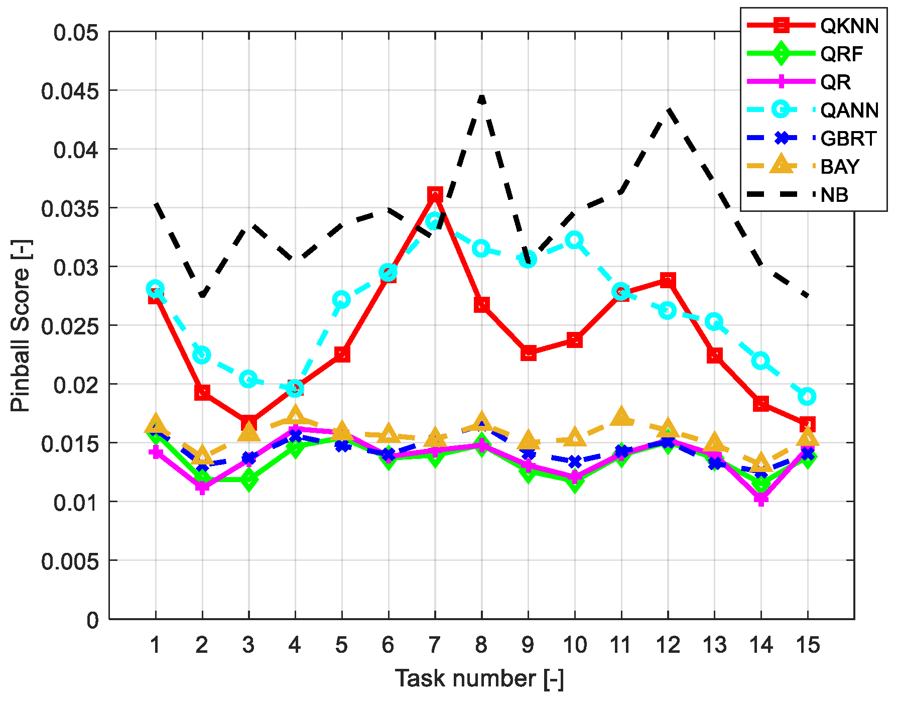
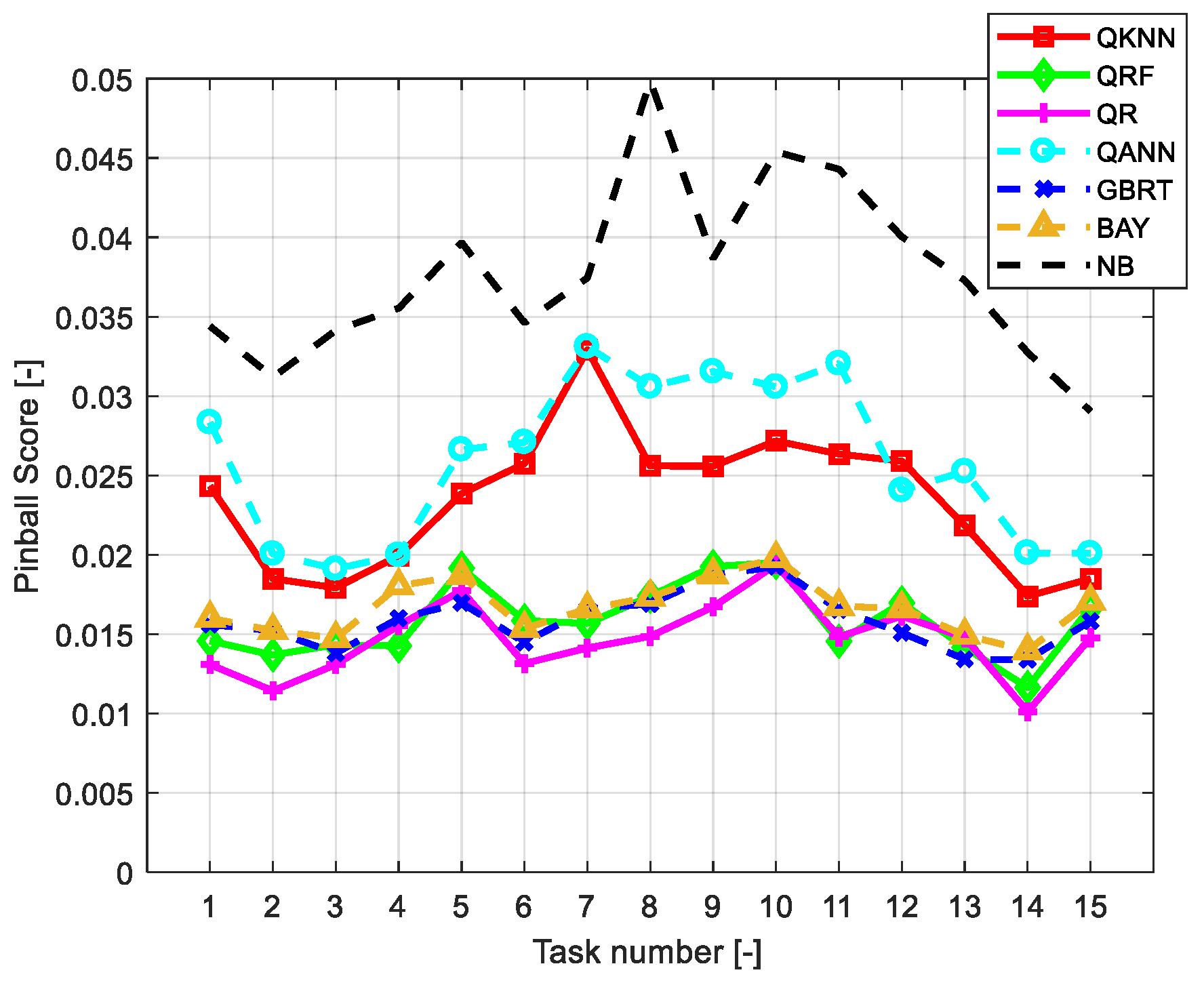
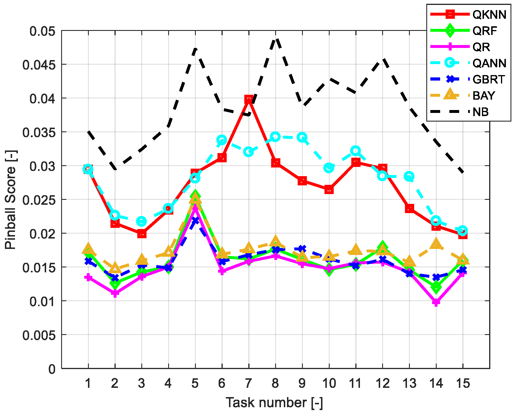
6.2. Assessment of the Accuracy of Individual Forecasts

We investigated the accuracy of the individual forecasts in all of the 15 tasks. The results during the last 5 tasks were also used as benchmarks, to compare the performances of the forecast combination approaches in the test step. Figure 2, Figure 3 and Figure 4 show the plots of the PSs obtained using the QKNN, the QRF, and the QR, to the 15 considered tasks, for the zones 1, 2, and 3, respectively. The benchmark PS values of the QANN, of the GBRT, of the BAY, and of the NB are also shown as a reference.

Figure 2, Figure 3 and Figure 4 clearly highlight the superior performances of QRF, QR, GBRT, and BAY models, with respect to the other models. For zone 1, QRF and QR perform very similarly, whereas for zones 2 and 3 the QR on average outperforms the QRF. The GBRT benchmark exhibits performances, on average, slightly worse than the QRF and QR; however, it outperforms the QANN and the QKNN for all of the zones considered. The BAY benchmark is, on average, slightly worse than the QRF, QR, and GBRT, whereas it outperforms QKNN, QANN, and NB.

Table 2. Pinball Score values averaged over tasks 11–15.

Method	Pinball Score [-]
	Zone 1	Zone 2	Zone 3
QKNN	0.0228	0.0220	0.0249
QRF	0.0136	0.0148	0.0152
QR	0.0136	0.0141	0.0139
QANN	0.0240	0.0243	0.0262
GBRT	0.0138	0.0149	0.0147
BAY	0.0153	0.0159	0.0169
NB	0.0349	0.0367	0.0376

shows the PS values of the individual forecasts and of the NB forecasts, averaged over tasks 11–15 (i.e., the tasks reserved for comparing the out-of-sample combination results). The PS values in Table 2 confirm the considerations made on the basis of the graphical inspection of Figure 2, Figure 3 and Figure 4.

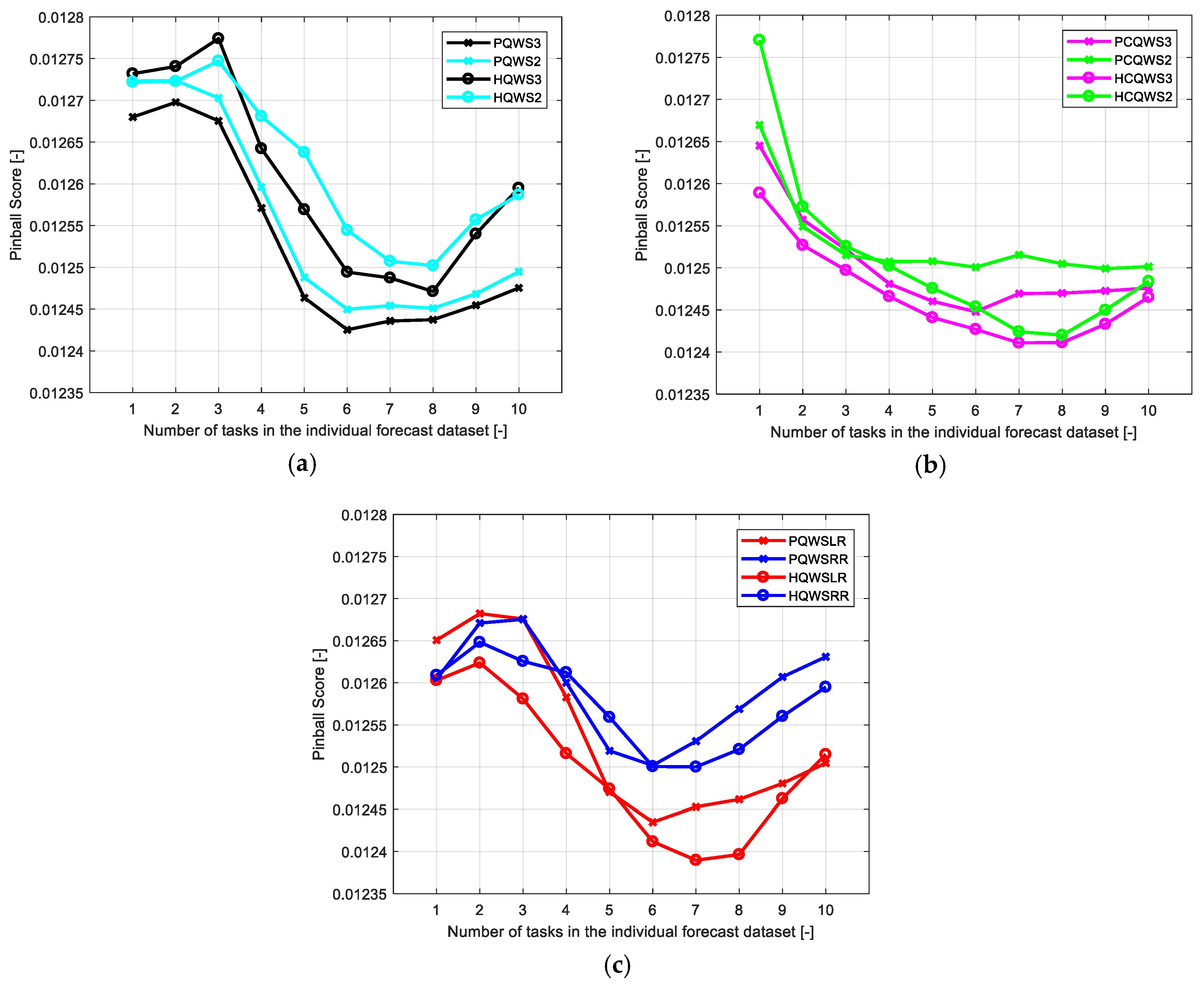
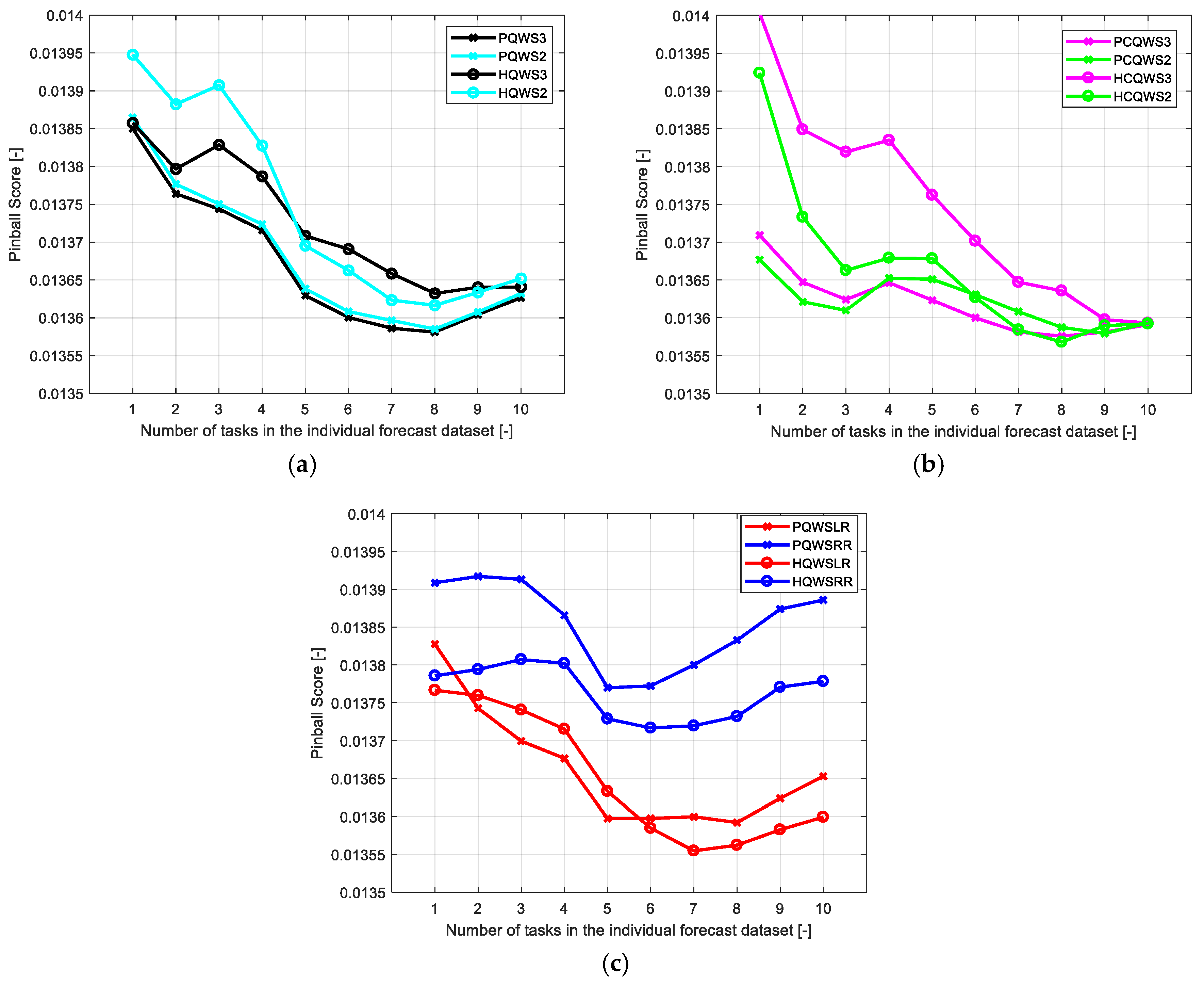
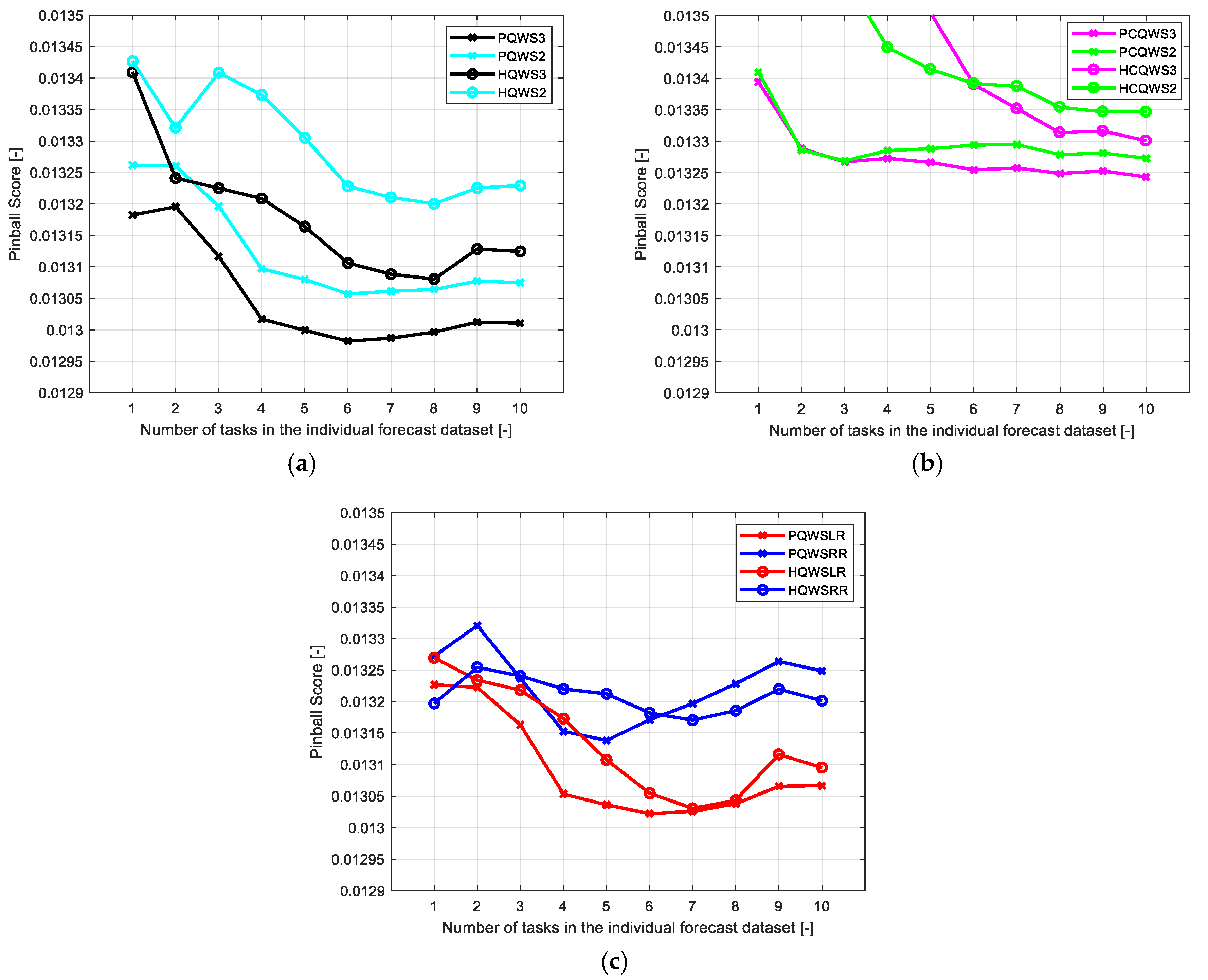
6.3. Assessment of the Accuracy of Combined Forecasts

PQWS2, PQWS3, HQWS2, HQWS3, PCQWS2, PCQWS3, HCQWS2, HCQWS3, PQWSLR, HQWSLR, PQWSRR, and HQWSRR forecasts are analyzed in this sub-Section. Different values of hyper-parameter $L$ (i.e., the length of the dataset used to train the weights of the combination models) are considered separately; in particular, they cover the 1, 2, …, 10 most recent tasks.

Figure 5, Figure 6 and Figure 7 show, for zones 1, 2, and 3, the PS values of the forecasts to the number of tasks considered to form the individual forecast dataset. In particular, Figure 5, Figure 6 and Figure 7a illustrate the PQWS2, PQWS3, HQWS2, HQWS3 results; Figure 5, Figure 6 and Figure 7b illustrate the PCQWS2, PCQWS3, HCQWS2, HCQWS3 results; and Figure 5, Figure 6 and Figure 7c illustrate the PQWSLR, HQWSLR, PQWSRR, HQWSRR results.

These figures clearly highlight that the PQWS3 outperforms the unconstrained, non-regularized strategies for all of the tasks considered. For zone 1, the HCQWS3 outperforms the other constrained strategies, whereas PCQWS3 performs better than the other constrained strategy for zone 3. Note, however, that the constrained strategies, compared to the unconstrained and regularized strategies, have quite similar results for zones 1 and 2, whereas the constrained strategies are definitely less accurate than the unconstrained and the regularized strategies for zone 3.

The smallest error score among all of the options considered is obtained for the zones 1 and 2 by using the HQWSLR with 7 tasks in the individual forecast dataset, whereas the best forecasts among all of the options considered for zone 3 are obtained through the PQWS3 with 6 tasks in the individual forecast dataset.

The trends of the PS of the combined forecasts are quite similar, as the performances significantly increase by using more than four tasks to form the individual forecast dataset; this improvement is at maximum around 6–8 tasks, and it slightly decreases with more tasks.

Altogether, the PQWS approaches outperform the HQWS ones, thus a more general model works better than a model with too much differentiation in the unconstrained, non-regularized estimation. Things change when the weight estimation is subject to constraints or to regularization; the hourly differentiation improves the performances of the forecasting ensemble for zones 1 and 2.

We now analyze in detail the best competitors for the three zones: the HQWSLR for zone 1 and 2, and the PQWS3 for zone 3. In particular, for both strategies we consider only the best-case scenario and the worst-case scenario, in terms of number of tasks in the individual forecast dataset. For the PQWS3, the optimal number of tasks selected to train upon the individual forecast datasets was 6, 8, and 6, for zones 1, 2, and 3, respectively; the worst performances of the PQWS3 were instead obtained with 2, 1, and 2 tasks for zones 1, 2, and 3, respectively. For the HQWSLR, the optimal number of tasks selected to train upon the individual forecast datasets was 7 for all of the zones; the worst performances of the HQWSLR were instead obtained with 2, 1, and 1 tasks for zones 1, 2, and 3, respectively.

The comprehensive

Table 3. Pinball Score values averaged over the tasks 11–15. Bold values highlight the best results for each zone.

Method	Pinball Score [-]
	Zone 1	Zone 2	Zone 3
QKNN	0.0228	0.0220	0.0249
QRF	0.0136	0.0148	0.0152
QR	0.0136	0.0141	0.0139
QANN	0.0240	0.0243	0.0262
GBRT	0.0138	0.0149	0.0147
BAY	0.0153	0.0159	0.0169
NB	0.0349	0.0367	0.0376
Best PQWS3	0.0124	0.0136	0.0130
Worst PQWS3	0.0127	0.0138	0.0132
Best HQWSLR	0.0124	0.0135	0.0130
Worst HQWSLR	0.0126	0.0138	0.0133

compares the corresponding PS values of these best- and worst-case scenarios to the ones obtained for the individual forecasts and for the benchmark (see Table 2). It is evident from these results that the forecast combination, either through the PQWS3 or the HQWSLR, always improves the skill of the forecasts.

We quantitatively assessed the results of the PQWS3 and of the HQWSLR by comparing them to the most competitive benchmarks for each zone, which are the QRF for the zone 1, and the QR for the zones 2 and 3. In the best-case scenario, the PS obtained through the PQWS3 is about 9%, 3.5%, and 6.5% smaller than the corresponding PS of the most competitive benchmark for zones 1, 2, and 3, respectively; in the worst-case scenario, the PS obtained through the PQWS3 is about 6.5%, 2%, and 5% smaller the corresponding PS of the most competitive benchmark for zones 1, 2, and 3, respectively. The improvement of the HQWSLR towards the most competitive benchmark for each zone is instead about 9%, 4.5%, and 6.5% in the best-case scenario, and about 7.5%, 2.5%, and 4.5% in the worst-case scenario, for zones 1, 2, and 3 respectively.

7. Conclusions

This paper discusses several strategies that have been developed to combine individual probabilistic PV power forecasts, aimed at building combined forecasts which are more accurate than individual predictions. Several types of combination strategies and architectures were developed in a competitive ensemble framework; all of them are based on the weighted quantile combination. The proposal was validated through numerical experiments based on PV power data published during the GEFCOM2014; several benchmarks are also presented, in order to compare the results.

The comparison of different forecast strategies for three different generation zones suggests that:

• the weighted quantile combination was effective in improving the accuracy of forecasts; it is able to outperform the accuracy of individual probabilistic forecasts, which is the main aim of competitive ensemble methods.
• The forecast combination improved the skill of the forecasts in all of the scenarios considered, with a reduction in terms of PS that is up to 9%.
• On average, the best results were obtained using the HQWSLR combination strategy for zones 1 and 2, and the PQWS3 combination strategy for the zone 3; the optimal length of the dataset used to train the weights of the combination models always ranges between 6 and 8 tasks.
• Adding the forecasts of an individual model which has worse performances than the other individual models appears to provide useful diversity in the ensemble approach; this appears to be valid both for unconstrained, non-regularized strategies and for constrained strategies.
• Adding too much dispersion to the forecast combination by estimating weights for each hour of the day does not improve the quality of the results for unconstrained, non-regularized regression; vice versa, constraints and/or regularization allow taking benefit from this hourly differentiation.

References

1. Toubeau, J.F.; Bottieau, J.; Vallee, F.; De Greve, Z. Deep learning-based multivariate probabilistic forecasting for short-term scheduling in power markets. IEEE Trans. Power Syst. 2018, 34, 1203–1215. [Google Scholar] [CrossRef]
2. Javadi, M.; Marzband, M.; Funsho Akorede, M.; Godina, R.; Saad Al-Sumaiti, A.; Pouresmaeil, E. A centralized smart decision-making hierarchical interactive architecture for multiple home microgrids in retail electricity market. Energies 2018, 11, 3144. [Google Scholar] [CrossRef]
3. Marzband, M.; Azarinejadian, F.; Savaghebi, M.; Pouresmaeil, E.; Guerrero, J.M.; Lightbody, G. Smart transactive energy framework in grid-connected multiple home microgrids under independent and coalition operations. Renew. Energy 2018, 126, 95–106. [Google Scholar] [CrossRef]
4. Capizzi, G.; Lo Sciuto, G.; Napoli, C.; Tramontana, E. Advanced and adaptive dispatch for smart grids by means of predictive models. IEEE Trans. Smart Grid 2018, 9, 6684–6691. [Google Scholar] [CrossRef]
5. Matos, M.; Bessa, R.J.; Botterud, A.; Zhou, Z. Forecasting and setting power system operating reserves. In Renewable Energy Forecasting: From Models to Applications, 1st ed.; Kariniotakis, G., Ed.; Woodhead Publishing: Duxford, UK, 2017; pp. 279–308. [Google Scholar]
6. Camal, S.; Michiorri, A.; Kariniotakis, G. Optimal offer of automatic frequency restoration reserve from a combined PV/wind virtual power plant. IEEE Trans. Power Syst. 2018, 33, 6155–6170. [Google Scholar] [CrossRef]
7. Carpinelli, G.; Mottola, F.; Proto, D. Probabilistic sizing of battery energy storage when time-of-use pricing is applied. Electr. Power Syst. Res. 2016, 141, 73–83. [Google Scholar] [CrossRef]
8. Van der Meer, D.W.; Widén, J.; Munkhammar, J. Review on probabilistic forecasting of photovoltaic power production and electricity consumption. Renew. Sustain. Energy Rev. 2018, 81, 1484–1512. [Google Scholar] [CrossRef]
9. Ren, Y.; Suganthan, P.N.; Srikanth, N. Ensemble methods for wind and solar power forecasting—A state-of-the-art review. Renew. Sustain. Energy Rev. 2015, 50, 82–91. [Google Scholar] [CrossRef]
10. Muralitharan, K.; Sakthivel, R.; Vishnuvarthan, R. Neural network based optimization approach for energy demand prediction in smart grid. Neurocomputing 2018, 273, 199–208. [Google Scholar] [CrossRef]
11. Alobaidi, M.H.; Chebana, F.; Meguid, M.A. Robust ensemble learning framework for day-ahead forecasting of household based energy consumption. Appl. Energy 2018, 212, 997–1012. [Google Scholar] [CrossRef]
12. Mangalova, E.; Agafonov, E. Wind power forecasting using the k-nearest neighbors algorithm. Int. J. Forecast. 2014, 30, 402–406. [Google Scholar] [CrossRef]
13. Shang, C.; Wei, P. Enhanced support vector regression based forecast engine to predict solar power output. Renew. Energy 2018, 127, 269–283. [Google Scholar] [CrossRef]
14. Tato, J.H.; Brito, M.C. Using smart persistence and random forests to predict photovoltaic energy production. Energies 2018, 12, 100. [Google Scholar] [CrossRef]
15. Bracale, A.; Carpinelli, G.; De Falco, P.; Hong, T. Short-term industrial reactive power forecasting. Int. J. Electr. Power Energy Syst. 2019, 107, 177–185. [Google Scholar] [CrossRef]
16. Hong, T.; Pinson, P.; Fan, S.; Zareipour, H.; Troccoli, A.; Hyndman, R.J. Probabilistic energy forecasting: Global energy forecasting competition 2014 and beyond. Int. J. Forecast. 2016, 32, 896–913. [Google Scholar] [CrossRef]
17. Hong, T. Energy forecasting: Past, present, and future. Foresight 2014, 32, 43–48. [Google Scholar]
18. Huang, J.; Perry, M. A semi-empirical approach using gradient boosting and k-nearest neighbors regression for GEFCom2014 probabilistic solar power forecasting. Int. J. Forecast. 2016, 32, 1081–1086. [Google Scholar] [CrossRef]
19. Almeida, M.P.; Perpiñán, O.; Narvarte, L. PV power forecast using a nonparametric PV model. Sola. Energy 2015, 115, 354–368. [Google Scholar] [CrossRef] [Green Version]
20. Bracale, A.; Carpinelli, G.; De Falco, P. A probabilistic competitive ensemble method for short-term photovoltaic power forecasting. IEEE Trans. Sustain. Energy 2017, 8, 551–560. [Google Scholar] [CrossRef]
21. Juban, R.; Ohlsson, H.; Maasoumy, M.; Poirier, L.; Kolter, J.Z. A multiple quantile regression approach to the wind, solar, and price tracks of GEFCom2014. Int. J. Forecast. 2016, 32, 1094–1102. [Google Scholar] [CrossRef]
22. Hong, T.; Pinson, P.; Fan, S. Global Energy Forecasting Competition 2012. Int. J. Forecast. 2014, 39, 357–363. [Google Scholar] [CrossRef]
23. Wang, Y.; Zhang, N.; Tan, Y.; Hong, T.; Kirschen, D.S.; Kang, C. Combining probabilistic load forecasts. IEEE Trans. Smart Grid 2018, in press. [Google Scholar] [CrossRef]
24. Golestaneh, F.; Pinson, P.; Gooi, H.B. Very short-term nonparametric probabilistic forecasting of renewable energy generation—With application to solar energy. IEEE Trans. Power Syst. 2016, 31, 3850–3863. [Google Scholar] [CrossRef]
25. Gneiting, T.; Raftery, A.E. Strictly proper scoring rules, prediction, and estimation. J. Am. Stat. Assoc. 2007, 102, 359–378. [Google Scholar] [CrossRef]
26. Møller, J.K.; Nielsen, H.A.; Madsen, H. Time-adaptive quantile regression. Comput. Stat. Data Anal. 2008, 52, 1292–1303. [Google Scholar] [CrossRef]
27. Ziel, F.; Liu, B. Lasso estimation for GEFCom2014 probabilistic electric load forecasting. Int. J. Forecast. 2016, 32, 1029–1037. [Google Scholar] [CrossRef] [Green Version]
28. Gaillard, P.; Goude, Y.; Nedellec, R. Additive models and robust aggregation for GEFCom2014 probabilistic electric load and electricity price forecasting. Int. J. Forecast. 2016, 32, 1038–1050. [Google Scholar] [CrossRef]
29. R Gbm Package: Generalized Boosted Regression Models. Available online: https://CRAN.R-project.org/package=gbm (accessed on 4 March 2019).
30. Bracale, A.; Carpinelli, G.; De Falco, P.; Rizzo, R.; Russo, A. New advanced method and cost-based indices applied to probabilistic forecasting of photovoltaic generation. J. Renew. Sustain. Energy 2016, 8, 023505. [Google Scholar] [CrossRef]
Figure 1. Overview of the proposed competitive ensemble method for forecasting photovoltaic (PV) power.
Energies 12 01011 g001
Figure 2. Pinball Score values of individual forecasts for zone 1.
Energies 12 01011 g002
Figure 3. Pinball Score values of individual forecasts for zone 2.
Energies 12 01011 g003
Figure 4. Pinball Score values of individual forecasts for zone 3.
Energies 12 01011 g004
Figure 5. Pinball Score values of combined forecasts for the zone 1: (a) PQWS2, PQWS3, HQWS2, and HQWS3 strategies; (b) PCQWS2, PCQWS3, HCQWS2, HCQWS3 strategies; (c) PQWSLR, HQWSLR, PQWSRR, HQWSRR strategies.
Energies 12 01011 g005
Figure 6. Pinball Score values of combined forecasts for the zone 2: (a) the Pure Quantile Weighted Sum (PQWS)2, PQWS3, Hourly Quantile Weighted Sum (HQWS)2, and HQWS3 strategies; (b) Pure Constrained Quantile Weighted Sum (PCQWS)2, PCQWS3, Hourly Constrained Quantile Weighted Sum (HCQWS)2, HCQWS3 strategies; (c) Pure Quantile Weighted Sum with Least Absolute Shrinkage and Selection Operator (LASSO) Regularization (PQWSLR), Hourly Quantile Weighted Sum with LASSO Regularization (HQWSLR), Pure Quantile Weighted Sum with Ridge Regularization (PQWSRR), Hourly Quantile Weighted Sum with Ridge Regularization (HQWSRR) strategies.
Energies 12 01011 g006
Figure 7. Pinball Score values of combined forecasts for the zone 3: (a) PQWS2, PQWS3, HQWS2, and HQWS3 approaches; (b) PCQWS2, PCQWS3, HCQWS2, HCQWS3 approaches; (c) PQWSLR, HQWSLR, PQWSRR, HQWSRR approaches.
Energies 12 01011 g007