Optimal Sizing of Cascade Hydropower and Distributed Photovoltaic Included Virtual Power Plant Considering Investments and Complementary Benefits in Electricity Markets

Abstract

Due to an imminent fossil energy crisis and environmental pollution, renewable energy, such as photovoltaics, has been vigorously developing. However, the output of photovoltaic energy has strong volatility and intermittency. Thus, the photovoltaic generation system cannot constantly meet the load demand. To address this problem, a virtual power plant with hydro-photovoltaic-thermal generation is proposed in this paper. This virtual power plant utilizes the complementary characteristics of the output of the power sources to ensure a smooth and stable total output curve, and the power supply quality of the virtual power plant is improved. Further, the nonlinear operating cost model of the virtual power plant, with output changing over time, is established on the weighted output of hydro, photovoltaic, and thermal power; then, the corresponding marginal cost model of the virtual power plant is obtained. In the electricity market, three typical mid- to long-term electricity decomposition methods based on average, tracking load and spot price are constructed, and the spot price is predicted by the auto regressive moving average model (ARIMA) model, while the relationship between the spot price and the marginal cost of the virtual power plant is obtained; the marginal cost could also be adjusted based on the ARIMA model. Based on above factors, the sizing model of the virtual power plant is established, considering investment and complementary benefits. Finally, a case study is undertaken, where the sizing scheme for the increasing local load in the typical scenarios of the planning year and the corresponding annual rate of return are obtained. Sensitivity analysis of the influence for the above factors on the sizing of the virtual power plant is carried out. The optimal ratio of mid- to long-term electricity and its decomposition methods, as well as the capacity of the virtual power plant and the sizing ratio of hydropower, photovoltaic, and thermal power are obtained.

1. Introduction

Considering the depletion of fossil energy, such as oil and coal, and the elimination of environmental pollution, the energy crisis is required to be solved by alternative clean energy sources [1]. Renewable energy, such as photovoltaic energy, is a promising solution for continuous exploitation. 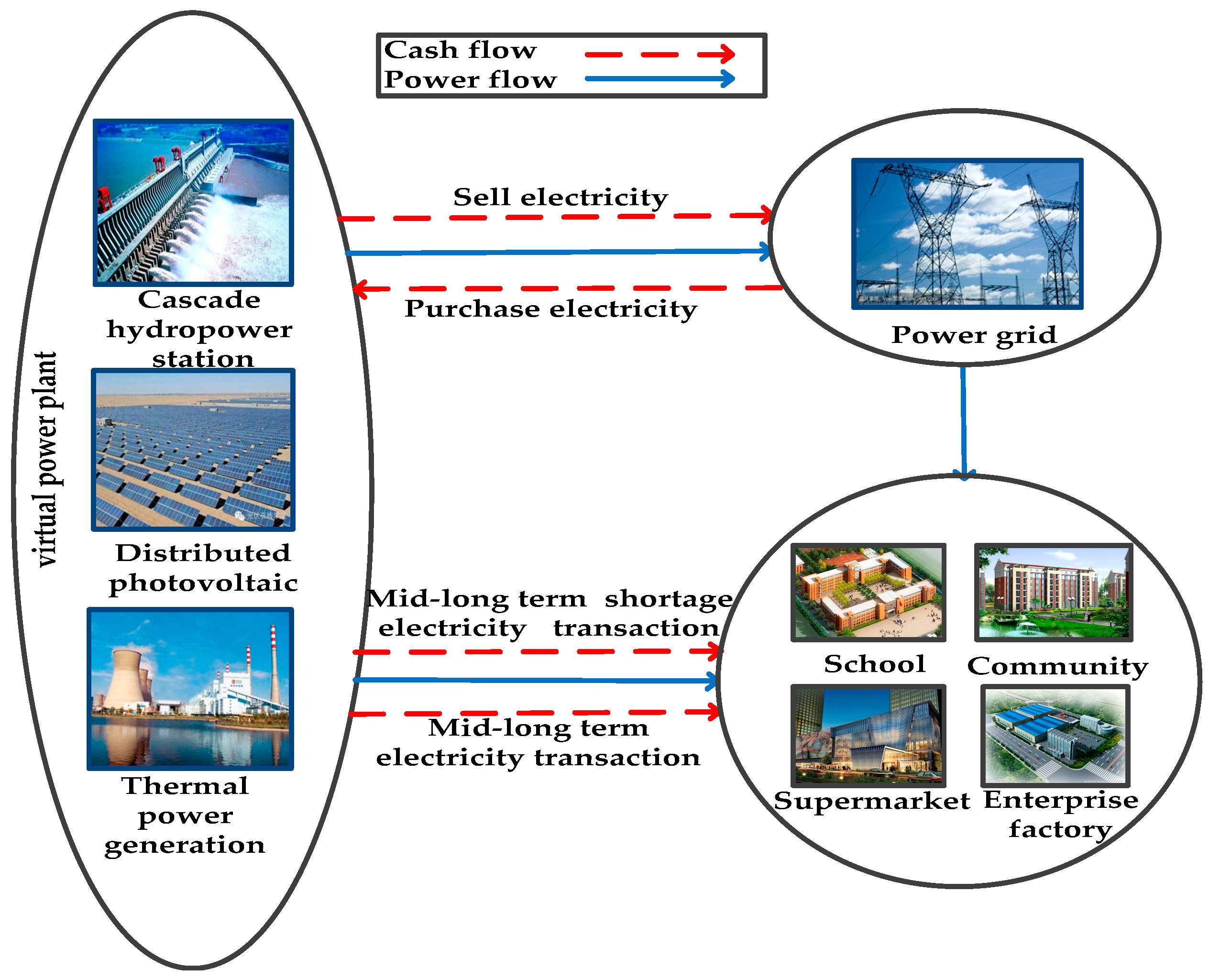However, due to the uncertain and intermittent output of renewable power generation, a single energy type cannot completely replace the role of traditional power plants in the power system [2]. A virtual power plant, including various power generating technologies, can improve the utilization and complementarity of various energy sources. For example, the volatility of photovoltaic output is complemented by a hydropower station, which has a fast response capability [3], while thermal power has better peak shaving performance. Therefore, a virtual power plant that includes hydropower, photovoltaic power, and thermal power could ensure a smooth and stable total power output curve, and the volatility of the renewable power generation system could be reduced when integrating to the grid, thereby improving the power supply quality [4].

At present, China has opened up the mid- to long-term power transaction market, and is working hard to promote the construction of the spot market in order to accelerate the reform of the electricity market. It is necessary to consider the interaction between the mid- to long-term market and the spot market. Particularly, the fluctuation of spot price, the electricity purchase ratio in two markets, and the decomposition of mid- to long-term electricity transactions bring significant challenges to the sizing of virtual power plants. For example, the high proportion of mid- to long-term electricity purchases could reduce the risk of price uncertainty in the spot market. However, a high spot price would restrict the profit margin of the virtual power plant. The lower the mid- to long-term electricity purchase ratio is, the more electricity would be exposed to the spot risk. In addition, with different decomposition modes, the electricity transaction’s curve would be different in the spot market; then, the purchase and sale of electricity would be affected in the spot market. Further, the profit from electricity sales and the cost from electricity purchases could be influenced by the matching degree between the spot electricity transaction’s curve and the spot price curve. Hence, the spot market’s risk could be effectively covered by the benefit gained from reasonable sizing planning for the virtual power plant.

There are limitations in different power supplies in the virtual power plant: The output of photovoltaic power has the randomness of its output greatly affected by light intensity [5]. The output of a hydropower station is restricted by the available water resources, which have a strong seasonal effect [6]. Therefore, the complementary effect of various power sources within a virtual power plant may not achieve the expected total output in different scenarios. Increasing the size of the virtual power plant would improve the capacity deployment and associated complementary effect of power supplies, while the investment cost would become an issue [7]. Therefore, by identifying the economic links and complementary effects between various power generating sources, together with a developed mutual constraint and coordinated operating strategy, the optimal sizing of the virtual power plant could make full use of the complementary between various power supplies, ensure the satisfaction of the total power output curve, enhance resource utilization, and achieve better economic profit in the electricity market.

So far, several studies on sizing and the economic operation of a virtual power plant with renewable energy have been done. In [8], a united dispatch center for a multi-energy generation system was proposed to obtain the appropriate sizing. The reasonable ratio of wind-photovoltaic to a conventional source was derived through multi-energy complementary characteristics, to achieve peak shift and high economics in [9]. Reference [10] researched the relationship between the cost-effectiveness and sizing of virtual power plants, and a sizing model based on economics and reliability combination was established. In [11], a virtual power plant including wind and photovoltaic power was analyzed in typical scenarios, and the sizing optimization model with the lowest investment cost and minimum power fluctuation was established. In [12], a sizing method for the virtual power plant based on a wavelet algorithm to suppress the randomness of short-term and long-term output of renewable energy was proposed. In [13], the characteristics of renewable energy were analyzed, and by using the complementarity of each energy source in time series, a hybrid renewable energy system, which improved energy utilization and social environment, was established. With large-scaled wind power integration, a unit commitment model was proposed to coordinate hydro and thermal power generation to support secure and economic wind power integration in [14]. In [15], by considering the unpredictable output characteristics of renewable energy, scheduling strategies for the virtual power plant were presented to determine the right balance between risks and benefits based on fuzzy chance-constrained scheduling model. In [16], the dependency between wind power and photovoltaic power was analyzed with the function copulas. Then, a sizing model for a multi-energy generation system was proposed to balance the cost and power fluctuation of wind and photovoltaic generation. In [17], a coordinated dispatch method with pumped-storage and battery-storage for compensating the variation of wind power was built to improve the safety issues for wind power systems. In [18], an optimal operation strategy for virtual power plants, based on demand response and game theory, was proposed. In [19], an optimal sizing strategy was proposed in the electricity spot market.

However, the above studies were insufficient to consider the planning and operation of a virtual power plant in an economic environment like the electricity market, particularly in both the mid- to long-term transaction market and the spot market. In this paper, the optimal sizing of the virtual power plant, considering the investment and complementary benefits for electricity market, is proposed. More specifically, this paper considers the electricity purchase ratio in mid- to long-term electricity, the decomposition method for mid- to long-term electricity transaction, the spot price uncertainty, and the convergence problems between long-term markets and the spot market. the economic and complementary coordination between these above factors on the sizing of virtual power plant are discussed.

The main contributions of the paper are as follows:

(1)

The output characteristic model of a virtual power plant is established by modeling each power source. The relationship and operating coordination between power supplies are studied to complement the intermittent photovoltaic output. The complementary evaluation indexes of the system are constructed to ensure a stable and controllable total power output curve from virtual power plant.

(2)

The operating cost model of virtual power plant and the marginal cost model are established based on the output ratio of each power source, which reflects the relationship intuitively between total output and operating cost, and the output is optimized by this.

(3)

In the electricity market, various typical mid- to long-term electricity decomposition methods were built, and the spot price was predicted by the auto regressive moving average model (ARIMA), and the correlation between output of virtual power plant and spot price was obtained.

(4)

Considering the above factors, the sizing model of a virtual power plant is proposed based on economic and complementary characteristics.

(5)

The rest of this paper is organized as followed. In Section 2, the output characteristic model of the virtual power plant and the complementary indexes of the virtual power plant are established. Section 3 represents the operating cost model of the virtual power plant. In Section 4, the sizing model of the virtual power plant in the electricity market is proposed. Section 5 represents the solution of the sizing method for the virtual power plant. In Section 6, numerical case studies verify the effectiveness of the proposed model. The conclusion is given in Section 7.

2. Output Characteristic Model of the Virtual Power Plant

The virtual power plant studied in this paper is composed of hydropower, thermal power and photovoltaic power. The flexibility of the short-term output of hydropower and the effective peak-shaving performance of thermal power can be used to compensate the random output of photovoltaic power [20].

In this work, the relationship between the virtual power plant, local load, and power grid is shown in Figure 1. The virtual power plant could sign a forward contract with the local load to trade electricity. This portion of electricity is settled as a mid- to long-term contract price to mitigate the risks from electricity price uncertainty. The rest-power demand for a local load is defined as a mid- to long-term shortage of electricity, which is settled at the spot market price. While meeting the local load demand, the surplus electricity of the virtual power plant would be exported to the power grid in the spot market. Oppositely, if the output of virtual power plant is insufficient to supply the local load, it is necessary to purchase electricity from power grid in the spot market.

2.1. Modeling of the Virtual Power Plant

2.1.1. Modeling of the Hydropower System

There is a time-lag relationship of water flow between the upper and lower stages of the hydropower stations. This time-lag means that the water flow from the upstream reservoir will flow into the downstream reservoir over a period of time. Then, the natural water quantity and reservoir water level constraints need to be considered for the model of cascade hydropower stations [21].

The amount of water available in a cascade hydropower basin is limited. The scheduling of a hydropower station at various time series is interrelated. The scheduling plan of the upper hydropower station would affect the water available for the lower-level hydropower stations to use, which would affect the overall dispatching plan. By considering the complex relationship between hydropower stations and the context of the scheduling for each time period, the model of hydropower stations is established [22]:

$$P_{hyd,i,t}=A{\eta }_i{H}_{i,t}{q}_{i,t}$$

(1)

where $P_{hyd,i,t}$ is the output of hydroelectric hydropower station $i$ at the period of $t$; the conversion coefficient $A$ between power and water is 0.0098, ${\eta }_i$ is the generation efficiency of the hydropower station $i$, $H_{i,t}$ is the hydrogen power generation head of the hydropower station $i$ at the period of $t$, and $q_{i,t}$ is the water flow of the hydropower station $i$ at the period of $t$.

Constraints of the hydropower station are as follows:

$$V_{i,t}=V_{i,t-1}+r_{i,t}-q_{i,t}-s_{i,t}+{\displaystyle \sum _{j\in U_i}(q_{j,t-{\tau }_j}+s_{j,t-{\tau }_j})}$$

(2)

$$V_{i,\min }\le V_{i,t}\le V_{i,\max }$$

(3)

$$q_{i,\min }\le q_{i,t}\le q_{i,\max }$$

(4)

$$P_{i,\min }\le P_{Hi,t}\le P_{i,\max }$$

(5)

where $V_{i,t}$ is the water quantity of the reservoir $i$ at the period of $t$, $r_{i,t}$ is the natural water quantity of the reservoir $i$ at the period of $t$, $q_{i,t}$ is the water flow of the hydropower station $i$ at the period of $t$, and $s_{i,t}$ is the abandoned water of the hydropower station $i$ at the period of $t$. $V_{i,t-1}$ is the water quantity of the reservoir $i$ at the period of $t-1$, $q_{j,t-{\tau }_j}$ is the water flow of the upstream hydropower station $j$ before ${\tau }_j$ hour, $s_{j,t-{\tau }_j}$ is the abandoned water of the upstream power station $j$ before ${\tau }_j$ hour, $V_{i,\min }$, and $V_{i,\max }$ are the respective minimum and maximum reservoir water volume of the upstream power station $i$. $q_{i,\min }$, $q_{i,\max }$ are the respective minimum and maximum water flow of the hydropower station $i$. $P_{i,\min }$, $P_{i,\max }$ are the minimum and maximum output of the hydropower station $i$.

2.1.2. Modeling of Distributed Photovoltaics

The output of distributed photovoltaic power is correlated with the light intensity and ambient temperature [23]. By taking the uncertainty into account, the total output model of distributed photovoltaic power is as follows:

$$P_{pv,t}={\displaystyle \sum _{i=1}^{n_{pv}}\{P_{pv,i}^m{\displaystyle \sum _{o=1}^O({\zeta }_{i,t}^o{L}_{AC,i,t}^o)}[1+}{k}_T(T_{c,i,t}-T_r)]/L_{stc}\}$$

(6)

$${\displaystyle \sum _{o=1}^O{\zeta }_{i,t}^o}=1$$

(7)

where ${\zeta }_{i,t}^o$ is the probability of the light intensity $L_{AC,i,t}^o$ at the period of $t$. $n_{pv}$ is the number of distributed photovoltaic power, $P_{pv,i}^m$ is the maximum output of distributed photovoltaic $i$ in a standard test environment, $k_T$ is the power-temperature coefficient; $T_{c,i,t}$ is the ambient temperature at the location of distributed photovoltaic $i$. The reference temperature ($T_r$) is 25 °C, and the test light intensity ($L_{stc}$) is 1000 W/m².

2.1.3. Modeling of Thermal Power System

The operating cost model of thermal power unit $i$ is as follow.

$$F_{the,i,t}=a_{the,i}{P}_{the,i,t}^2+b_{the,i}{P}_{the,i,t}+c_{the,i}$$

(8)

where $a_{the,i}$, $b_{the,i}$, $c_{the,i}$ are the coefficients of the thermal power unit $i$ operating cost model, and $P_{thei,t}$ is the output of the thermal power unit $i$ at the period of $t$.

Constraints of thermal power unit:

$$P_{the,i}^{\min }\le P_{thei,t}\le P_{the,i}^{\max }$$

(9)

$$\{\begin{array}{l}{P}_{Ti,t}-P_{Ti,t-1}\le \Delta tU{R}_{Ti}^{}\\ P_{Ti,t-1}-P_{Ti,t}\le \Delta tD{R}_{Ti}^{}\end{array}$$

(10)

where $P_{Ti}^{\min }$, $P_{Ti}^{\max }$ are the minimum and maximum output of unit $i$ respectively, where $\Delta t$ is the time interval in the scheduling period, and $U{R}_{Ti}^{}$, $D{R}_{Ti}^{}$ are the ramp-down limit and ramp-up limit of unit $i$ respectively.

2.2. The Complementary Indexes of the Virtual Power Plant

A virtual power plant with hydropower, photovoltaics, and thermal power utilizes the complementary characteristics among the various power supplies to ensure a smooth and stable output curve. The total power output is described as:

$${\displaystyle \sum _{t=1}^T{P}_{L,t}}={\displaystyle \sum _{i=1}^{n_{the}}{\displaystyle \sum _{t=1}^T{P}_{the,i,t}}}+{\displaystyle \sum _{i=1}^{n_{hyd}}{\displaystyle \sum _{t=1}^T{P}_{hyd,i,t}}}+{\displaystyle \sum _{i=1}^{n_{pv}}{\displaystyle \sum _{t=1}^T{P}_{pv,i,t}}}$$

(11)

where $n_{hyd}$ is the number of hydropower stations, $n_{the}$ is the number of thermal power units, and $T$ is the number of optimization period.

The amount of the change of hydropower, photovoltaic, and thermal power output is calculated as follows:

$$\begin{array}{c}{\alpha }_{hyd}^j=(P_{hyd}^{j+1}-P_{hyd}^j)\\ {\alpha }_{pv}^j=(P_{pv}^{j+1}-P_{pv}^j)\\ {\alpha }_{the}^j=(P_{the}^{j+1}-P_{the}^j)\end{array},j=1,2,\dots ,n-1$$

(12)

where ${\alpha }_{hyd}^j$, ${\alpha }_{pv}^j$, ${\alpha }_{the}^j$ are the changes of hydropower, photovoltaic respectively, $P_{hyd}^j$, $P_{pv}^j$, $P_{the}^j$ are sample values of the power output of hydropower, photovoltaic, and thermal power, respectively, and thermal power output, the time interval between each adjacent two sampling points is the same, and $n$ is the number of sampling points. The amount of the change of total power output ${\alpha }^j$ is as follows:

$${\alpha }^j={\alpha }_{hyd}^j+{\alpha }_{pv}^j+{\alpha }_{the}^j.$$

(13)

The virtual power plant coordinates hydropower and thermal power to complement the randomness of photovoltaic power, to ensure a smooth and stable output curve, by minimizing the rate of change of total power output as follows:

$$\left|\frac{{\alpha }^j}{\frac{1}{n}{\displaystyle \sum _{j=1}^n(P_{hyd}^j+P_{pv}^j+P_{the}^j)}}\le B_v\right|$$

(14)

$$\left|\frac{\min (P_{hyd}^j+P_{pv}^j+P_{the}^j)-\frac{1}{n}{\displaystyle \sum _{j=1}^n(P_{hyd}^j+P_{pv}^j+P_{the}^j)}}{\frac{1}{n}{\displaystyle \sum _{j=1}^n(P_{hyd}^j+P_{pv}^j+P_{the}^j)}}\right|\le B_g$$

(15)

$$\left|\frac{\max (P_{hyd}^j+P_{pv}^j+P_{the}^j)-\frac{1}{n}{\displaystyle \sum _{j=1}^n(P_{hyd}^j+P_{pv}^j+P_{the}^j)}}{\frac{1}{n}{\displaystyle \sum _{j=1}^n(P_{hyd}^j+P_{pv}^j+P_{the}^j)}}\right|\le B_f$$

(16)

where $B_v$, $B_f$, $B_g$ are the ratio of change of total power output curve, and the respective upper and lower limits.

3. Operating Cost Model of the Virtual Power Plant

The virtual power plant studied in this paper includes hydropower stations, distributed photovoltaics, and thermal power, in which hydropower stations and photovoltaics have no operating costs [24].

In order to reflect the relationship between the total output, and operating cost for the optimal scheduling of the virtual power plant, the operating cost model can be expressed as the following function

$$F_L=f(P_L).$$

(17)

The operating cost is proposed as a non-linear quadratic function model with the ratio of hydropower, photovoltaics, and thermal power output at each period.

$$F_L={\displaystyle \sum _{t=1}^T{F}_{L,t}}={\displaystyle \sum _{t=1}^T(a_{L,t}{P}_{L,t}{}^2+b_{L,t}{P}_{L,t}+c_{L,t})}$$

(18)

where, $P_L$ is the total output of the virtual power plant, $F_{L,t}$ is the operating cost of the virtual power plant at the period of $t$, and $a_{L,t}$, $b_{L,t}$, $c_{L,t}$ are the respective coefficients of the operating cost model. To solve the model coefficients, the following method is proposed.

Firstly, consider that the operating cost is equal to the thermal power unit operating cost, as follows:

$$a_{L,t}{({\displaystyle \sum _{i=1}^{n_{hyd}}{P}_{hyd,i,t}}+{\displaystyle \sum _{i=1}^{n_{the}}{P}_{the,i,t}}+{\displaystyle \sum _{i=1}^{n_{pv}}{P}_{pv,i,t}})}^2+b_{L,t}({\displaystyle \sum _{i=1}^{n_{hyd}}{P}_{hyd,i,t}}+{\displaystyle \sum _{i=1}^{n_{the}}{P}_{the,i,t}}+{\displaystyle \sum _{i=1}^{n_{pv}}{P}_{pv,i,t}})+c_{L,t}={\displaystyle \sum _{i=1}^{n_{the}}(a_{the,i}{P}_{the,i,t}{}^2+b_{the,i,t}{P}_{the,i,t}+c_{the,i,t})}$$

(19)

To map the quadratic part, the corresponding terms on both sides of the equation are equal, and the following formula is obtained:

$$a_{L,t}{({\displaystyle \sum _{i=1}^{n_{hyd}}{P}_{hyd,i,t}}+{\displaystyle \sum _{i=1}^{n_{the}}{P}_{the,i,t}}+{\displaystyle \sum _{i=1}^{n_{pv}}{P}_{pv,i,t}})}^2={\displaystyle \sum _{i=1}^{n_{the}}(a_{the,i}{P}_{the,i,t}{}^2)}$$

(20)

$$b_{L,t}({\displaystyle \sum _{i=1}^{n_{hyd}}{P}_{hyd,i,t}}+{\displaystyle \sum _{i=1}^{n_{the}}{P}_{the,i,t}}+{\displaystyle \sum _{i=1}^{n_{pv}}{P}_{pv,i,t}})={\displaystyle \sum _{i=1}^{n_{the}}(b_{the,i,t}{P}_{the,i,t})}$$

(21)

$$c_{L,t}={\displaystyle \sum _{i=1}^{n_{the}}{c}_{the,i,t}}.$$

(22)

In order to express the operating cost according to the power output ratio of hydropower, thermal power, and photovoltaic power, the output of one of thermal power units at the period of $t$ is set as benchmark, the output (p.u.) of the hydropower station, distributed photovoltaics, and thermal power units are respectively proposed as follows:

$${\lambda }_{hyd,i,t}=\frac{P_{hyd,i,t}}{P_{the,B,t}}$$

(23)

$${\lambda }_{pv,i,t}=\frac{P_{pv,i,t}}{P_{the,B,t}}$$

(24)

$${\lambda }_{the,i,t}=\frac{P_{the,i,t}}{P_{the,B,t}}.$$

(25)

Combining Equations (18)–(25), the coefficients of the operating cost model for the virtual power plant are as follows:

$$a_{L,t}=\frac{{\displaystyle \sum _{i=1}^{n_{the}}{a}_{the,i}{\lambda }_{the,i,t}^2}}{{({\displaystyle \sum _{i=1}^{n_{hyd}}{\lambda }_{hyd,i,t}}+{\displaystyle \sum _{i=1}^{n_{the}}{\lambda }_{the,i,t}}+{\displaystyle \sum _{i=1}^{n_{pv}}{\lambda }_{pv,i,t}})}^2}$$

(26)

$$b_{L,t}=\frac{{\displaystyle \sum _{i=1}^{n_{the}}{b}_{the,i}{\lambda }_{the,i,t}}}{({\displaystyle \sum _{i=1}^{n_{hyd}}{\lambda }_{hyd,i,t}}+{\displaystyle \sum _{i=1}^{n_{the}}{\lambda }_{the,i,t}}+{\displaystyle \sum _{i=1}^{n_{pv}}{\lambda }_{pv,i,t}})}.$$

(27)

Furthermore, the power output and marginal cost of the virtual power plant at the period of $t$ are obtained as follows:

$$P_{L,t}=({\displaystyle \sum _{i=1}^{n_{hyd}}{\lambda }_{hyd,i,t}+{\displaystyle \sum _{i=1}^{n_{the}}{\lambda }_{the,i,t}}+}{\displaystyle \sum _{i=1}^{n_{pv}}{\lambda }_{pv,i,t}})P_{the,B,t}$$

(28)

$$Z_{L,t}=2a_{L,t}{P}_{L,t}+b_{L,t}.$$

(29)

Once a relationship has been established between the operating cost output of the virtual power plant, the output and plant mix can be optimized to achieve the defined objective in operating cost. It is worth noting that the coefficients of the operating cost model would change with the mixed ratio of hydropower/photovoltaics/thermal power in a different period. Therefore, the operating cost model of the virtual power plant is assumed to be a nonlinear quadratic function that changes over time.

4. Sizing Model of the Virtual Power Plant in the Electricity Market

In the electricity market, based on different mid- to long-term electricity decomposition methods and spot price uncertainty, the sizing model of the virtual power plant, while considering investment and complementary benefits, is established.

4.1. Mid- to Long-Term Electricity Decomposition Method

The ratio of mid- to long-term electricity and its decomposition method would directly affect the purchase and sale of electricity, its profit, and its cost in the spot market, which in turn would affect the economics of sizing.

The mid- to long-term transaction contract is signed with a local load in the mid- to long-term transaction market:

$$P_{V,t}^{}=P_{v,t}^{}+P_{M,t}^{}$$

(30)

where $P_{M,t}^{}$ is the mid- to long-term electricity at the period of $t$, $P_{V,t}^{}$ is the actual local demand at the period of $t$, $P_{v,t}^{}$ is mid- to long-term shortage electricity at the period of $t$. Mid- to long-term electricity is settled as the mid- to long-term price, and the mid- to long-term shortage of electricity is settled at the spot price. A certain percentage of the local load should be selected to sign the mid- to long-term contracts. The remaining load demand will be met as the mid- to long-term shortage of electricity. The profit margin of the virtual power plant could be effectively improved, with the risk of mid- to long-term electricity deviation assessment effectively being avoided. The sizing of the virtual power plant would be affected by the decomposition method of mid- to long-term contracts, which typically includes the following three methods. The total mid- to long-term electricity in one day is known; electricity would be decomposed into various time periods by the following three methods.

4.1.1. Average Decomposition at Each Period

$$P_{M,t}=\frac{P_M}{T}$$

(31)

where $P_M$ is total mid- to long-term electricity in one day, $P_M$ is decomposed into various time periods ($T$); with this decomposition method, the mid- to long-term electricity curve trend of each period is the most stable.

4.1.2. Tracking Load Curve Decomposition

$$P_{M,t}=P_{V,t}\frac{P_M}{P_V}$$

(32)

where $P_V$ is the total electricity demand of the local load in one day; the mid- to long-term electricity at each time period would follow the load curve change with this decomposition method.

4.1.3. Decomposed by Spot Price

$$k^i=\frac{{\pi }_t}{{\displaystyle \sum _{t=1}^T{\pi }_t}}$$

(33)

where ${\pi }_t$ is the predicted spot price at the period of $t$; from Equation (31), the values of $k^i$ could be calculated, and they are sorted from small to large: $k_{}^1$, $k_{}^2$, $k_{}^3$…; The spot prices at various points are arranged from low to high, and the corresponding mid- to long-term decomposition amounts are ranked as the spot prices are arranged from low to high, and the corresponding mid- to long-term decomposition of electricity is obtained, $P_{M,t}^1$, $P_{M,t}^2$, $P_{M,t}^3$…,

$$P_{M,t}^j=k_{}^i{P}_M\begin{array}{cc}& (i+j=T+1)\end{array}$$

(34)

where $P_{M,t}^{}$ is the mid- to long-term decomposition electricity at each period. The mid- to long-term electricity at each period with this decomposition method is closely related to the spot price. The higher the spot price is, the lower the amount of mid- to long-term decomposition of electricity is. The lower the spot price is, the higher the amount of mid- to long-term decomposition of electricity is.

4.2. Analysis of the Uncertainty of Spot Price

In the day-ahead spot market, the virtual power plant would face the high risk caused by the uncertainty of the spot price, the prediction of the spot price is particularly important [25]. The accuracy of prediction would directly affect the economics of sizing.

The electricity price sequence in the spot market is a random time series. Through the extraction and analysis of historical electricity prices, the auto regressive integral moving average model ARIMA is used to predict the spot price [26]. The prediction model of spot price is as follows:

$${\pi }_t={\displaystyle \sum _{w=1}^W\left[{\zeta }_t^w(e_t+{\phi }_1{\pi }_{t-1}^w+{\theta }_1{\pi }_{t-1}^w+{\epsilon }_t)\right]}$$

(35)

$${\epsilon }_t~N(0,{\delta }_t^2)$$

(36)

$${\displaystyle \sum _{w=1}^W{\zeta }_t^w}=1$$

(37)

where ${\zeta }_t^w$ is the probability that the price is ${\pi }_t^w$ at the period of $t$, considering the uncertainty, ${\pi }_t$ is the expected value of the predicted spot price at the period of $t$; $e_t$ is the average price of the historical electricity prices; ${\phi }_1$ is the auto regressive coefficient of the electricity price sequence, ${\theta }_1$ is the moving average coefficient; ${\delta }_t^2$ is the variance of the electricity price series that changes over time; the expected value ${\epsilon }_t$ of the historical electricity prices is 0.

Based on the historical data of the spot market, the predicted spot price model can be solved. The predicted spot price is obtained in the day ahead spot market.

4.3. Sizing Model of the Virtual Power Plant

Considering the mid- to long-term electricity ratio and its decomposition, spot price uncertainty, and local load growth rate based on meeting the economic and complementary indexes of a virtual power plant, the sizing model for typical scenarios in the planning level year can be established.

The sizing scheme in year $y$ is as follows,

$$S^y=\left\{S_1^y,S_2^y,S_3^y,\dots \right\}.$$

(38)

The elements in the scheme are a system sizing in year $y$, and the annual yield of the virtual power plant, which is as follows:

$$\max r^y=\frac{R^y-F^y}{(Q_{the}^y{c}_{the}+Q_{hyd}^y{c}_{hyd}+Q_{pv}^y{c}_{pv})}$$

(39)

$$R^y={\displaystyle \sum _{l=1}^L\left\{D^l\left[{\displaystyle \sum _{t=1}^T({\pi }_{M,t}^{y,l}{P}_{M,t}^{y,l}+{\pi }_t^{y,l}{P}_{v,t}^{y,l}+{\pi }_t^{y,l}{\varphi }_t^{y,l}{P}_{\varphi ,t}^{y,l})}\right]\right\}}$$

(40)

$$F^y={\displaystyle \sum _{l=1}^L\left\{D^l\left[{\displaystyle \sum _{t=1}^T({\pi }_t^{y,l}{\mu }_t^y{P}_{\mu ,t}^{y,l}+F_{L,t}^{y,l})}\right]\right\}}$$

(41)

$$P_{L,t}^{y,l}=P_{M,t}^{y,l}+P_{v,t}^{y,l}+{\varphi }_t^{y,l}{P}_{\varphi ,t}^{y,l}-{\mu }_t^{y,l}{P}_{\mu ,t}^{y,l}$$

(42)

where $r^y$ is the rate of return in year $y$, $R^y$ is the revenue of the system in year $y$, $F^y$ is the sum of the total operating cost of the virtual power plant and the cost of purchasing electricity in year $y$, $F_{L,t}^{y,l}$ is the operating cost of the virtual power plant in period $t$ in typical scenarios; $l$ in year $y$, $c_{hyd}$, $c_{pv}$, $c_{the}$ are, respectively, the unit investment cost of hydropower, distributed photovoltaics, and thermal power units. $Q_{hyd}^y$, $Q_{pv}^y$, $Q_{the}^y$ are, respectively, the capacity deployment of hydropower, photovoltaic power, and thermal power in year $y$. $L$ is the number of typical scenes in one year. $D^l$ is the number of days of a typical scene $l$. $P_{L,t}^{y,l}$, $P_{V,t}^{y,l}$, $P_{v,t}^y$, $P_{\varphi ,t}^{y,l}$, $P_{\mu ,t}^y$ are, respectively, total output, local load demand, mid- to long-term shortage electricity, electricity sales, and the purchase of electricity in period $t$ in a typical scene $l$ in year $y$. ${\pi }_{M,t}^{y,l}$, ${\pi }_t^{y,l}$ are, respectively, the mid- to long-term price and spot price in a typical scene $l$ in year $y$. ${\varphi }_t^{y,l}$, ${\mu }_t^{y,l}$ are, respectively, the electricity purchase behavior and sales electricity behavior in a typical scene $l$ in year $y$.

In the future, considering the capacity deployment of hydropower units, photovoltaics and thermal power should be increased with the local load increasing. The model is established as follows:

$$P_{V,t}^{y,l}={(1+{\gamma }^{y,l}\%)}^y{P}_{V,t}^{0,l}$$

(43)

$$Q_{hyd}^y={(1+x_{hyd}^y\%)}^y{Q}_{hyd}^0$$

(44)

$$Q_{pv}^y={(1+x_{pv}^y\%)}^y{Q}_{pv}^0$$

(45)

$$Q_{the}^y={(1+x_{the}^y\%)}^y{Q}_{the}^0$$

(46)

where $P_{V,t}^{0,l}$ is local load demand in period $t$ in a typical scene $l$ in the horizontal year. $P_{V,t}^{y,l}$ is the local load demand in period $t$ in a typical scene $l$ in the $y$ year. ${\gamma }^{y,l}$ is the load growth rate in a typical scene $l$ in year $y$. $Q_{hyd}^0$, $Q_{pv}^0$, $Q_{the}^0$ are, respectively, the capacity deployment of hydropower, photovoltaics, and thermal power in the horizontal year. $x_{hyd}^y$, $x_{pv}^y$, $x_{the}^y$ are, respectively, the capacity deployment growth rate of hydropower, thermal power, and photovoltaic power in year $y$.

In the electricity market, firstly, the output of the virtual power plant should be larger than the mid- to long-term electricity. Then, it is necessary to optimize the output of the virtual power plant by adjusting the marginal cost on the spot price in the spot market; further, the purchase and sale of electricity must be obtained. The following constraints can be obtained:

$$P_{L,t}^y\ge P_{M,t}^y$$

(47)

$$Z_{L,t}^{y,l}\le {\pi }_{L,t}^{y,l}$$

(48)

$${\varphi }_t^{y,l}=\{\begin{array}{cc}1& P_{L,t}^{y.l}\ge P_{V,t}^y\\ 0& P_{L,t}^{y,l}<P_{V,t}^y\end{array}$$

(49)

$${\mu }_t^{y,l}=\{\begin{array}{cc}0& P_{L,t}^{y.l}\ge P_{V,t}^y\\ 1& P_{L,t}^{y,l}<P_{V,t}^y\end{array}$$

(50)

where $Z_{L,t}^{y,l}$ is the marginal cost, when $P_{L,t}^{y,l}<P_{V,t}^{y,l}$, ${\mu }_t^{y,l}$ is 1, to meet the local load demand during this period, the virtual power plant needs to purchase electricity from the day-ahead spot market. When $P_{L,t}^{y,l}>P_{V,t}^{y,l}$, ${\mu }_t^{y,l}$ is 1, the rest generated electricity of the virtual power plant could be sold in the day-ahead spot market.

The above nonlinear optimization model was performed using the professional optimization software, LINGO. By considering the mid- to long-term electricity ratio and its decomposition method and spot price, the optimized output of the virtual power plant and the sizing scheme and its corresponding annual rate of return based on economic and complementary characteristics are all obtained.

5. Sizing Method of the Virtual Power Plant

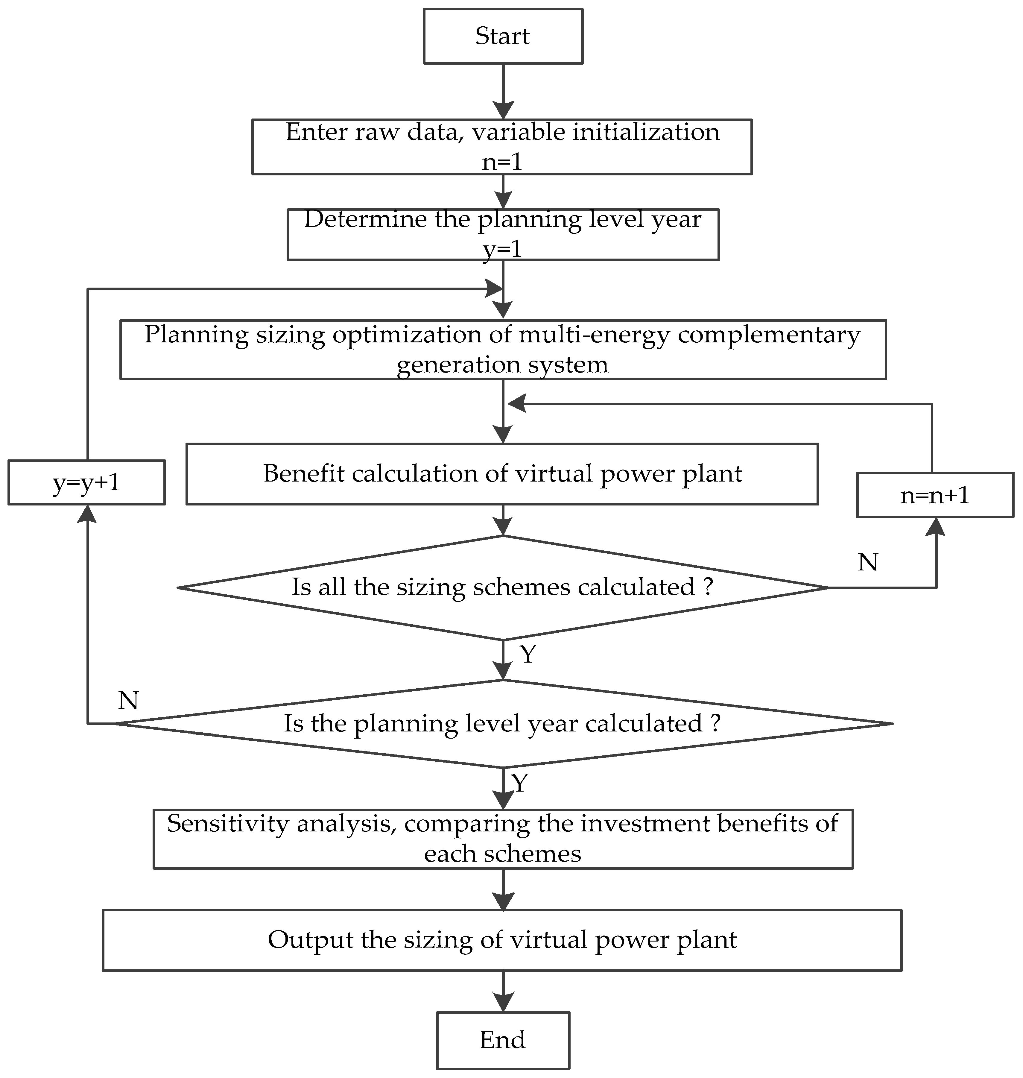
Within the increasing local load, this paper proposes a scheme set of sizing. Based on the output characteristic model of the virtual power plant in Equations (1)–(16), the operating cost model in Equations (17)–(29), the different mid- to long-term Equations electricity ratio and its decomposition methods in Equations (30)–(34), and the prediction model of spot price in Equations (35)–(37), the sizing model in Equations (38)–(50), which takes maximum annual profits and expected complementary indexes as its objective function, is established. Using this model, the rates of return for different schemes are all obtained. In contrast to these rates of return, the best scheme could be found in this planning set. The sizing flowchart is shown in Figure 2.

The specific process of the sizing is shown as follows:

• Input initial parameters include base load, hydropower, photovoltaics, and thermal power, complementary operation capacity deployment data, the parameters of the virtual power plant and its complementary indexes in Equations (11)–(16), the spot price, and the mid- to long-term price.
• Sizing of virtual power plant. The sizing scheme set is determined in Equation (38), according to the local load increase rate Equation (43) in a planning year.
• The rate of return for the sizing scheme in the set should be computed and contrasted against them.
• After calculating the rate of return, the sensitive analysis of some important parameters, such as the capacity deployment of hydropower, photovoltaic, and thermal power complementarity, different complementary modes, mid- to long-term contract price, spot market price, and mid- to long-term electricity ratio and its decomposition, need to be completed to derive their respective impact on the rate of return.
• Based on the contrast of rates of return for different sizing, the best scheme should be determined from a comprehensive consideration of economics and complementary effect.

In order to obtain the rate of return for every sizing scheme, first, the typical scenarios should be established according to the historical data of light intensity, water flow, mid- to long-term electricity price, spot market, etc. Then, considering other important factors, including different complementary indexes and operating costs, the mid- to long-term electricity ratio and its decomposition, the rate of return for every sizing could be derived from the system analog operation in typical scenarios. This process is shown as follows:

(1)

Input planning year data, such as load demand, thermal unit data, photovoltaic data, including light intensity and temperature, cascade hydropower stations installed, and storage capacity.

(2)

Calculate the investment cost of capacity deployment with a determined scheme in planning year.

(3)

According to the model of the virtual power plant in Equations (1)–(16), the virtual system source cost model in Equations (17)–(29), different mid- to long-term electricity ratio and its decomposition methods in Equations (30)–(34), and prediction model of spot price in Equations (35)–(37) calculate the rate of return.

(4)

Determine whether all sizing schemes are calculated. If all calculations are done, go to next step. Otherwise, return to step 2.

(5)

Output all the sizing results and corresponding rates of return.

6. Case Study

Considering the different ratios of mid-long term electricity and its decomposition methods, the operating cost of the virtual power plant, and the uncertainty of the spot price, with local load growing year by year in the planning cycle, the sizing scheme of the virtual power plant, based on economy and characteristic indexes, is obtained in this case study.

The virtual power plant is composed of three cascade hydropower stations, six thermal power units, and distributed photovoltaics. Parameters of hydropower stations, thermal power units and photovoltaic panels are respectively shown in

Table 1. Parameters of hydropower stations.

Number	Min Storage Capacity (104 m3)	Max Storage Capacity (104 m3)	Min Flow (m3/s)	Max Flow (m3/s)	Water Head (m)	Power Generation Efficiency
1	75.4	143.1	13.2	165.4	156.5	0.80
2	66.2	116.1	11.5	140.2	144.5	0.85
3	54.6	104.1	10.3	135.5	112.3	0.85

,

Table 2. Parameters thermal power units.

Number	aT ($/MW2h)	bT ($/MWh)	cT ($/h)	Pmax (MW)	Pmin (MW)	URi (MW/h)	DRi (MW/h)
1	0.002	19	260	600	130	110	110
2	0.0024	18	240	550	120	95	95
3	0.0026	16	210	500	100	90	90
4	0.0032	15	180	450	80	80	80
5	0.0036	14	175	350	70	60	60
6	0.004	13	160	300	50	50	50

and

Table 3. Parameters of photovoltaic panels.

Reference Temperature (°C)	Temperature Coefficient	Test Light Intensity (W/m2)
25	−0.5%	1000

. Finally, the sizing with the maximum investment benefit, based on the complementary indexes, is solved, and the system sizing scheme set in the planning cycle is obtained.

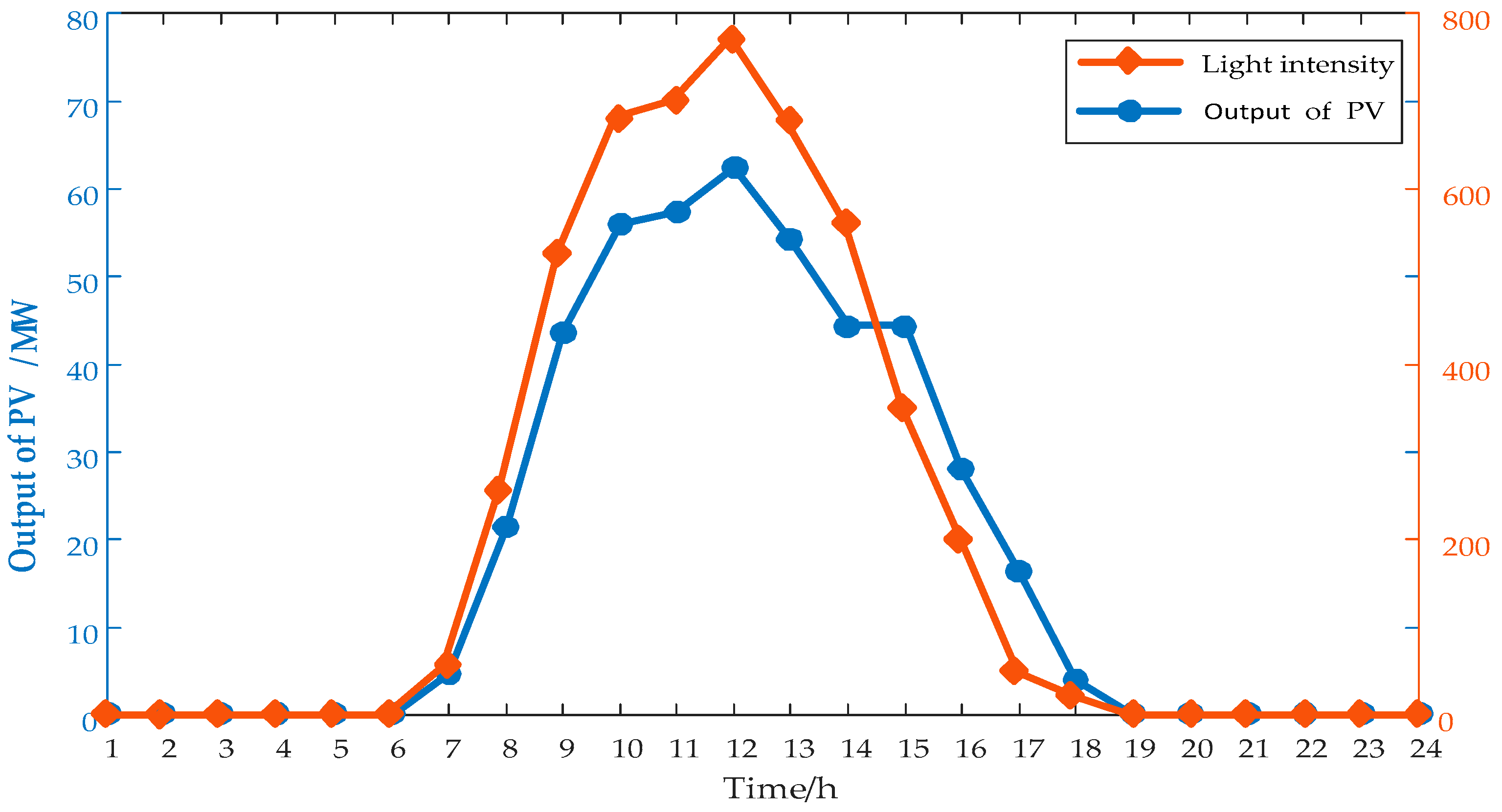
6.1. Predicted Output of Photovoltaics

As can be seen from Figure 3, the light intensity of the day changes constantly. The volatility of the output is larger, and at noon the output reaches its maximum. On the other hand, in this picture, the trend of the output of photovoltaics is basically consistent with the trend of changes in light intensity. The output of photovoltaic power is greatly affected by light intensity. The virtual power plant utilizes a wide range of outputs of the cascade hydropower station and the flexible adjustment capability of the thermal power to compensate for the output of photovoltaic power, so that the complementary effect of the system output is improved and the system power supply cooperability is enhanced

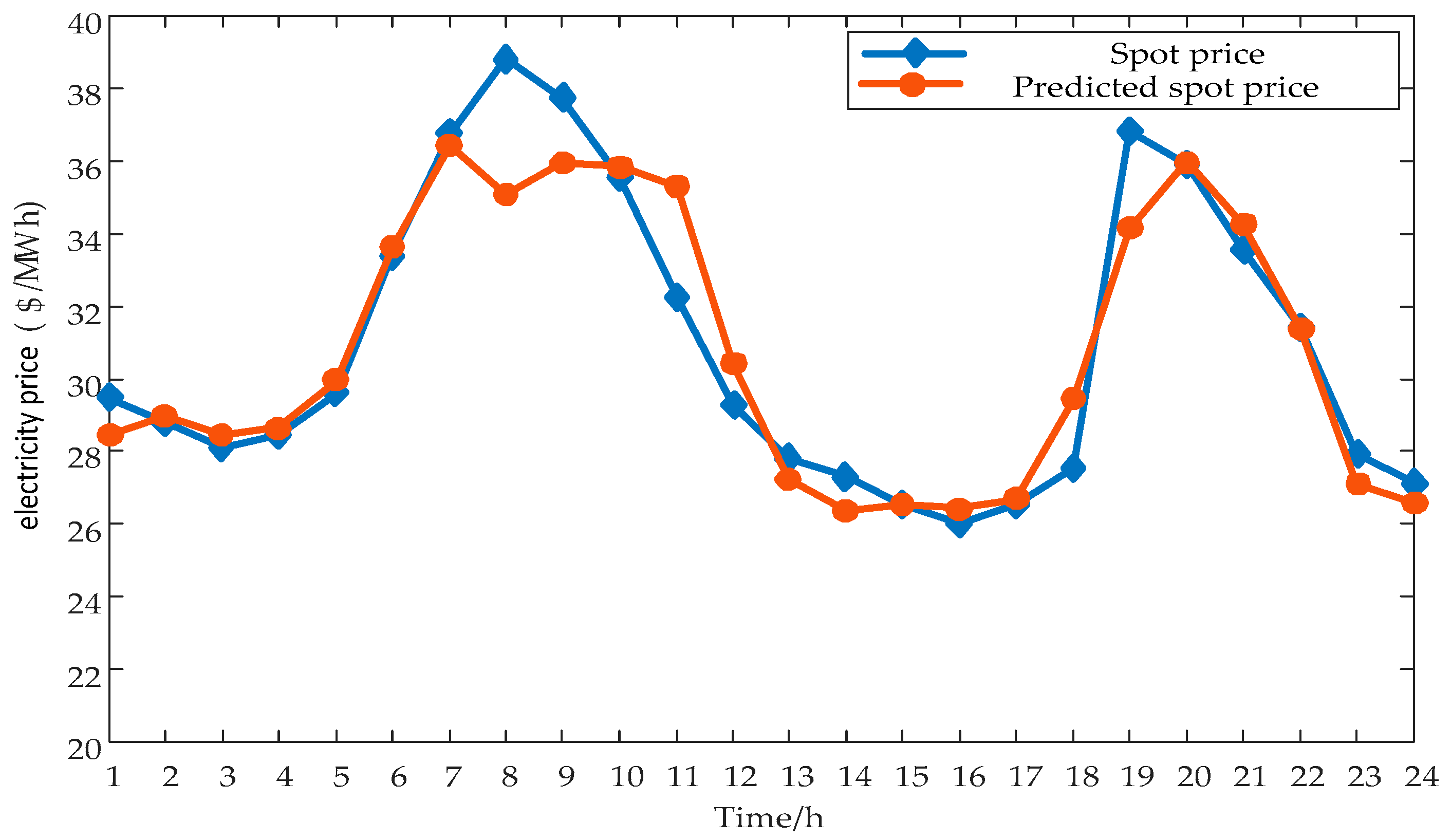
6.2. Prediction of Spot Price

In the electricity spot market, huge risks to market transactions are created by sharp fluctuations in spot prices, so the accuracy of a predicted spot price is very important. In this case, the 1632 spot prices of the California spot market from 1 January 2018 to 24 March 2018 were used as historical data to predict the spot price. The predicted spot price is shown in the following Figure 4. the predicted spot price curve is basically consistent with the true spot price curve, which confirms the accuracy of the method.

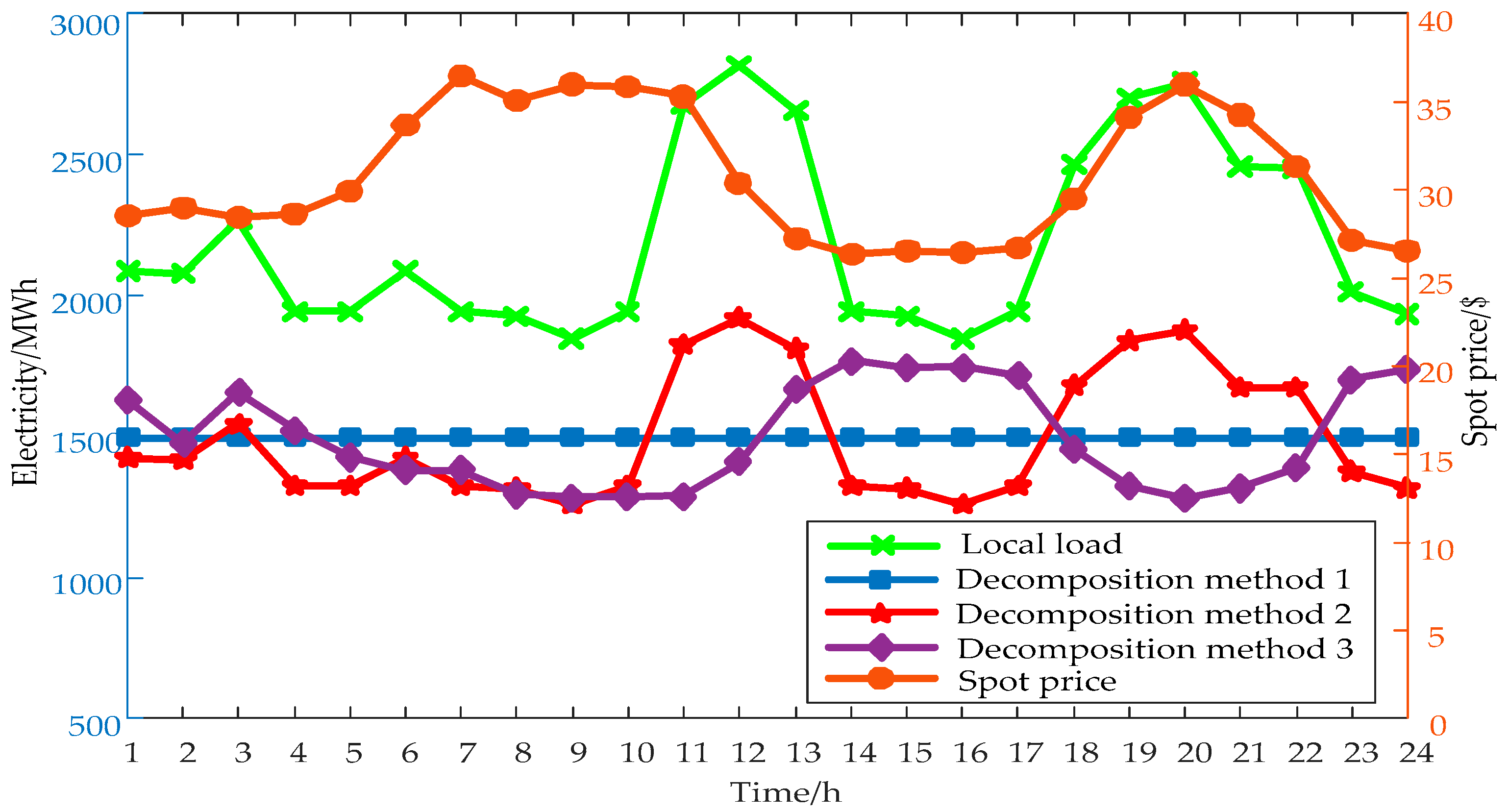
6.3. Three Typical Mid- to Long-Term Electricity Decomposition Curves

In the electricity market, the connection between the mid- to long-term market and the spot market is important. If the mid- to long-term price is stable, the spot market risk can be partly avoided through the mid- to long-term market. At the same time, with the decomposition method of mid- to long-term electricity, the long-term shortage of electricity and the spot price of electricity would be different at each period. The complementary indexes of the source end of the virtual power plant are $B_v$ = 0.15, $B_f$ = 0.18, $B_g$ = 0.15; 75% of the local load is mid- to long-term electricity. The mid- to long-term electricity with the three typical decomposition methods is shown in Figure 5.

As described in Figure 5, the mid- to long-term electricity curves with different decomposition modes have different trends. The space between the local load curve and mid- to long-term electricity curve is the mid- to long-term shortage electricity. There is a significant change in the amount of shortage electricity with different decomposition modes.

Decomposition method 1 is that the mid- to long-term electricity is decomposed evenly into each time period. This method is the simplest, and the mid- to long-term electricity in each period is the same. With decomposition method 2, the mid- to long-term electricity is decomposed by following the local load curve. If the shape of both curves is similar, the mid- to long-term shortage of electricity in this mode remains unchanged. With decomposition method 3, the mid- to long-term electricity is decomposed based on the spot price. This decomposition method is the most complicated. The mid- to long-term electricity curve is related to the predicted spot price, and the trend of the mid- to long-term electricity curve obtained in this mode is opposite to the predicted spot price curve. The higher the spot price is in a certain period, the less mid- to long-term electricity would be decomposed. At this time, more electricity would be sold at a higher spot price. Conversely, the lower the spot price is in a certain period, the more mid- to long-term electricity would be decomposed. At this time, the sale of low-price electricity is reduced.

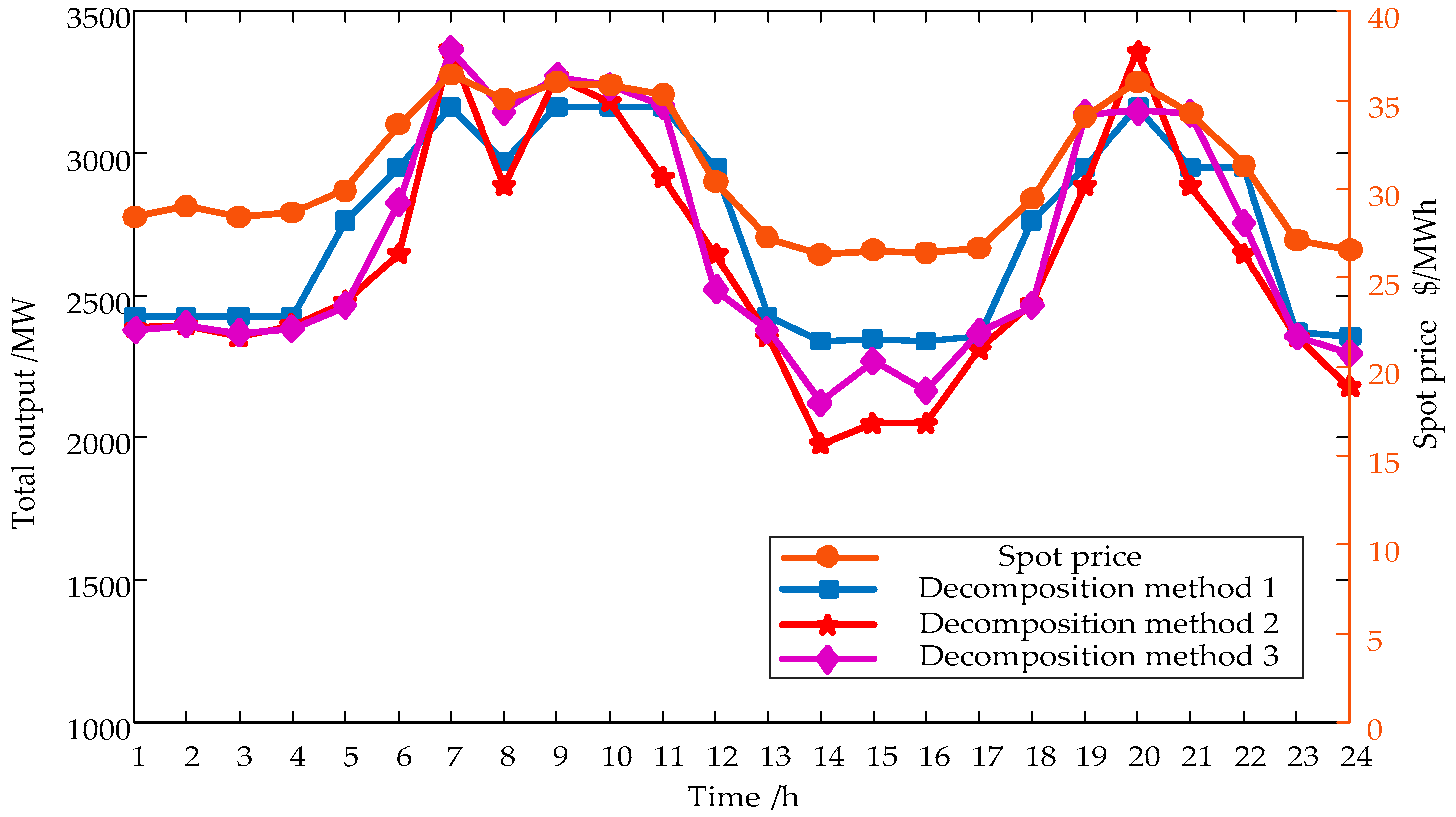
6.4. Characteristics of Output in the Spot Market

It is necessary that generated electricity of the virtual power plant is more than the mid- to long-term decomposition electricity in each period. Three different mid- to long-term decomposition methods are chosen, based on the relationship between the marginal cost of the virtual power plant and the spot price. The output was optimized until the marginal cost was equal to the spot price. The output curve of the virtual power plant and the three decomposition modes obtained are shown in Figure 6 below.

As shown in Figure 6, the trend of the output curve is basically consistent with the trend of the spot price curve. The higher the spot price is, the higher the output would be, which reflects the correlation between output and spot price. However, the output curve of the virtual power plant in each mode differs slightly.

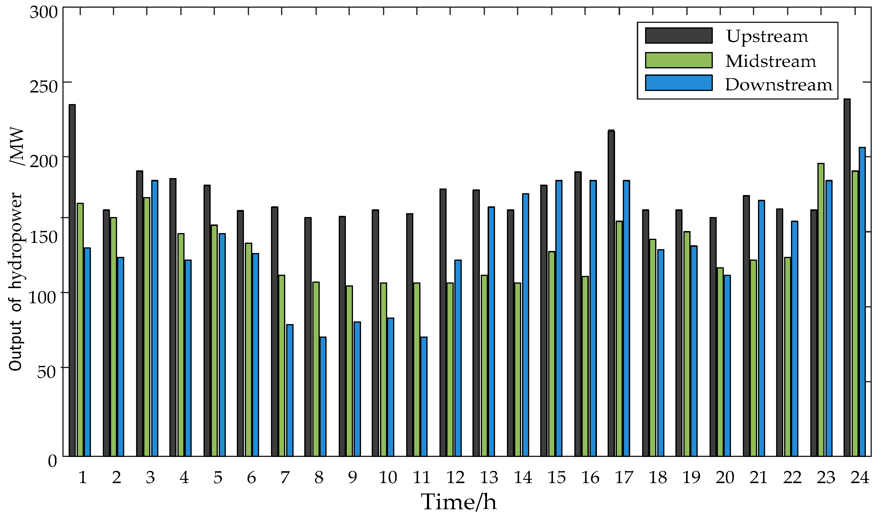
6.5. The Impact of Hydropower, Photovoltaic, Thermal Power Output Ratio on Profit

The virtual power plant is composed of cascade hydropower stations, thermal power units, and distributed photovoltaics. The total output of each part of the virtual power plant in each period constantly changes, so the operating cost of the virtual power plant would be changed synchronously; in this way, the profit would be affected. The complementary characteristic indexes of the virtual power plant are $B_v$ = 0.15, $B_f$ = 0.18, and $B_g$ = 0.15. The ratio of mid- to long-term electricity is 0.75, and the mid- to long-term electricity is decomposed according to method 3. The output of the hydropower station is attained, as shown in Figure 7. It can be seen that there is a correlation among the output of hydropower stations at all levels, and because the three cascade hydropower stations have storage capacity, they have certain adjustment capabilities.

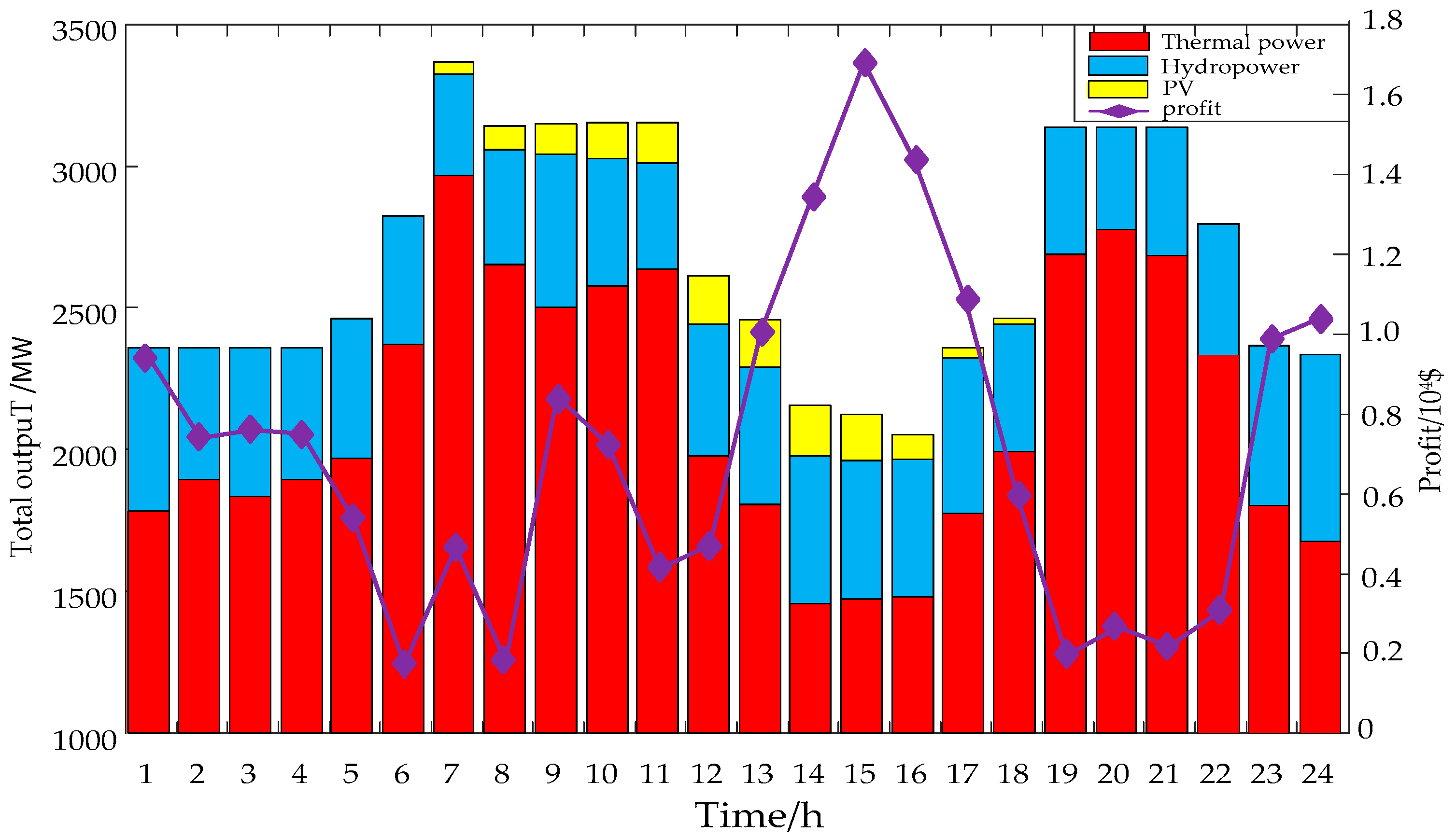
The total output of hydropower, photovoltaics, and thermal power at various time periods and their corresponding profits are shown in Figure 8. The output of photovoltaics, hydropower, and thermal power change constantly in various periods.

In Figure 8, it can be found that when the output of hydropower and photovoltaics change in each period, there is a significant impact on system profit, and the ratio of output in each period is different. When the output of hydropower and photovoltaics accounts for a relatively high proportion, the profit is relatively large. For example, between the eighth and ninth period, the total output of the virtual power plant was relatively stable. As the output of hydropower and photovoltaics increases, the profit shows a clear upward trend.

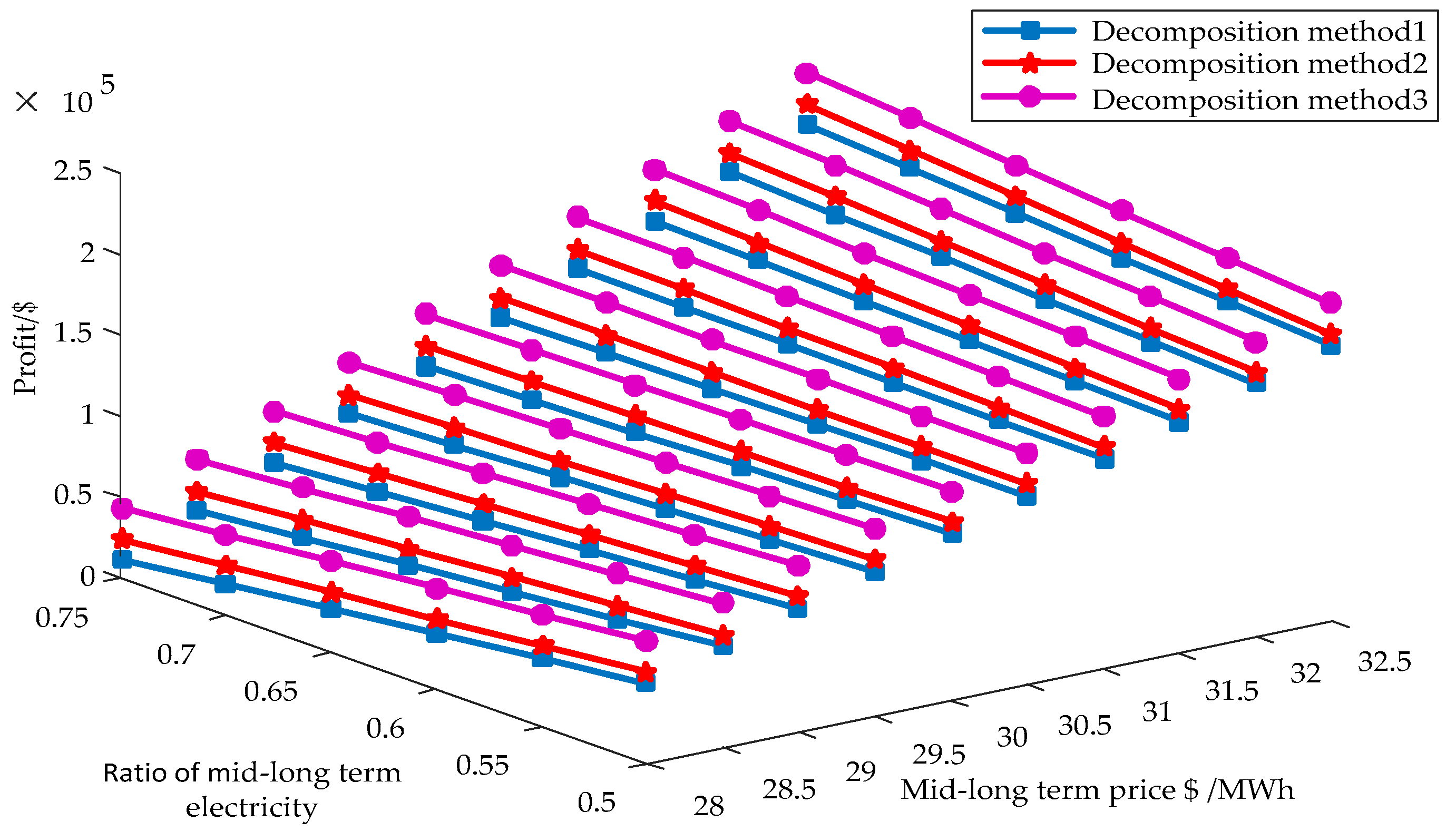
6.6. The Impact of Different Mid- to Long-Term Prices on Profit

Profit is closely related to the electricity price. To increase system profit while avoiding the risk of a virtual power plant, the ratio of mid- to long-term electricity and its decomposition methods needs to be selected based on a comprehensive consideration of mid- to long-term price and spot price. The profits of different mid- to long-term electricity ratios and their decomposition methods are shown in

Table 4. Profits with different mid- to long-term ratios and decompositions ($).

Mid- to Long-Term Electricity Price ($30.5/MWh)
Mid- to Long-Term Ratio α	Decomposition Method 1	Decomposition Method 2	Decomposition Method 3
0.50	1073856	1140375	1290034
0.55	1073040	1148685	1303119
0.60	1072225	1157110	1316383
0.65	1071409	1165654	1329829
0.70	1073040	1177004	1346531
0.75	1069777	1183110	1357283

and

Table 5. Profits with different mid- to long-term ratio and decompositions ($).

Mid- to Long-Term Electricity Price (30 $/MWh)
Mid- to Long-Term Ratio α	Decomposition Method 1	Decomposition Method 2	Decomposition Method 3
0.50	950327	1016847	1213742
0.55	936304	1011948	1204128
0.60	922111	1006997	1189191
0.65	907747	1001993	1177168
0.70	895248	999213	1165307
0.75	878485	991819	1153606

. while the mid- to long-term price is changed, the relationship between the profit and the ratio of mid- to long-term electricity is also different, as found in Figure 9.

It can be seen from Table 4 and Table 5, and Figure 9 above, that when the mid- to long-term price is low, the profit decreases as the proportion of mid- to long-term electricity increases. There are significant differences in the profit of systems with different mid- to long-term electricity ratios and their decomposition modes. In Table 5, the mid- to long-term price is $30.5/MWh, and with decomposition mode 1, the profit of the virtual power plant decreases with an increase in the ratio of mid- to long-term electricity, but with the decomposition mode 2 and decomposition mode 3, the profit of system increases with the ratio of the mid- to long-term electricity increasing, and the profit obtained is the highest with the decomposition mode 3; when the mid- to long-term electricity prices are different, the relationship between the profit of the system and the mid- to long-term ratio is be changed accordingly. For example, when the mid- to long-term price is $30/MWh, the profit would decrease as the mid- to long-term ratio increased.

With different mid- to long-term decomposition methods, the linear relationship among the profit and the ratio of the mid- to long-term price is shown in Figure 9. It can be seen that when the mid- to long-term price is low, the profit of the system decreases proportional to the mid- to long-term electricity increasing. When the mid- to long-term price is high, the profit of virtual power plant increases proportional to the mid- to long-term electricity increasing. This result is mainly determined by the mid- to long-term decomposition method and its mid- to long-term electricity price and spot price. With a certain mid- to long-term decomposition mode, and when the mid- to long-term price is high, a higher ratio of mid- to long-term electricity should be selected.

6.7. Analysis of Sizing Based on Economic and Complementary Indexes

The complementary indexes of the output carve are, respectively, $B_v$ = 0.15, $B_f$ = 0.18, $B_g$ = 0.15; the mid- to long-term electricity is decomposed on spot price, and the mid- to long-term electricity price is $30.5/MWh. The ratio of mid- to long-term electricity is selected as 0.75. The investment and complementary benefits of the virtual power plant are analyzed with different sizing ratios of hydropower, photovoltaics, and thermal power in the horizontal year. The specific sizing ratio is shown in

Table 6. Sizing ratio of hydropower, photovoltaic power, and thermal power.

Mode	Hydropower	PV	Thermal Power
ratio 1	17.50%	2.50%	80%
ratio 2	25%	5.00%	70%
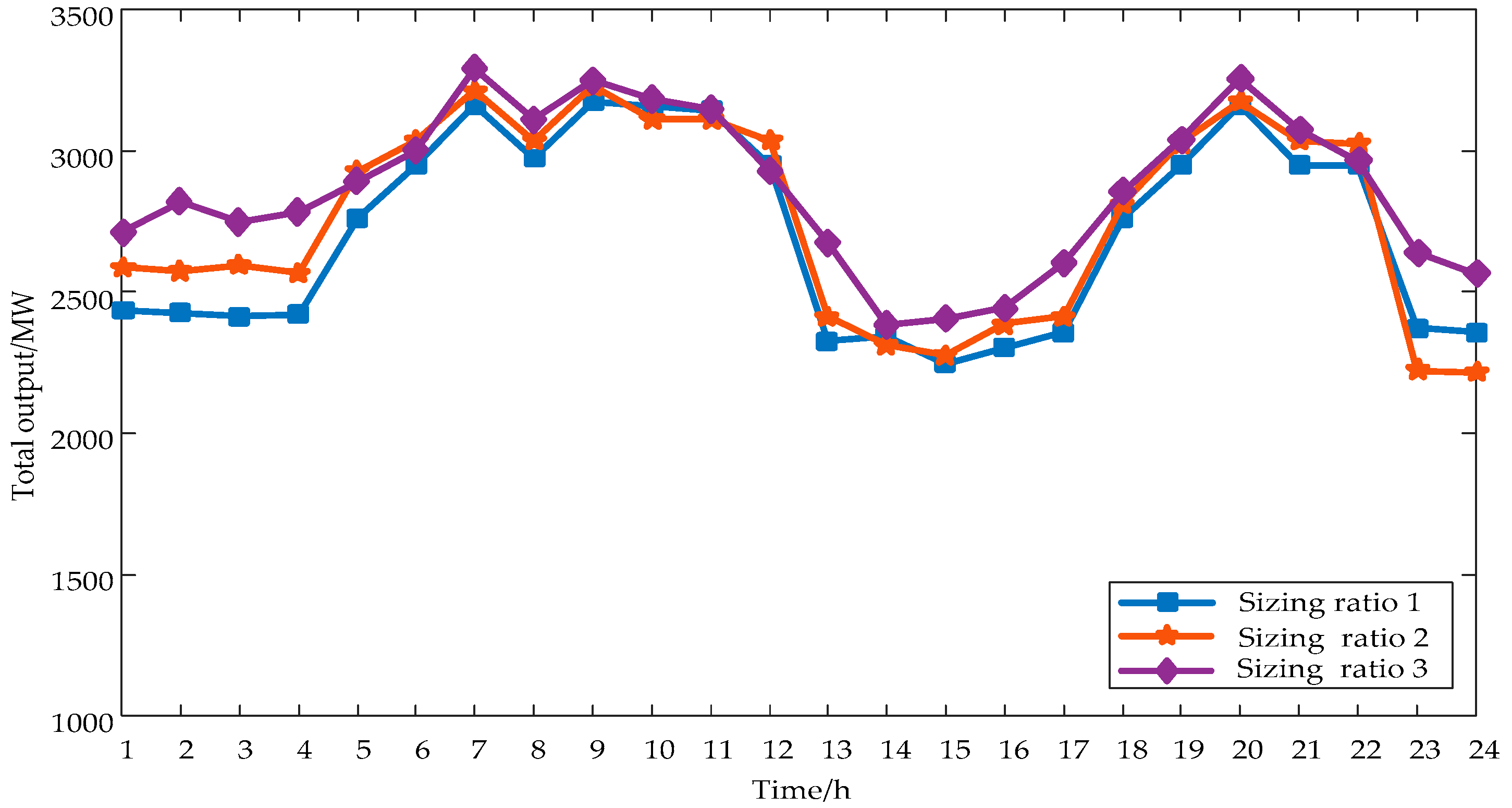
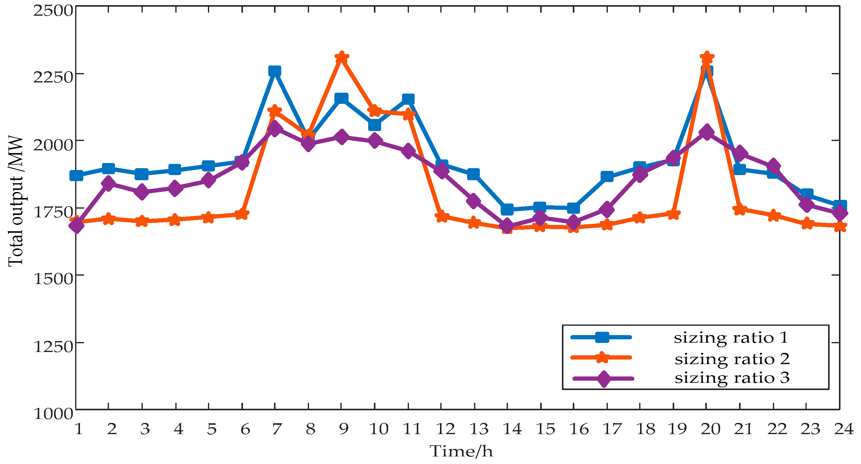
ratio 3	35%	7.50%	57.5%

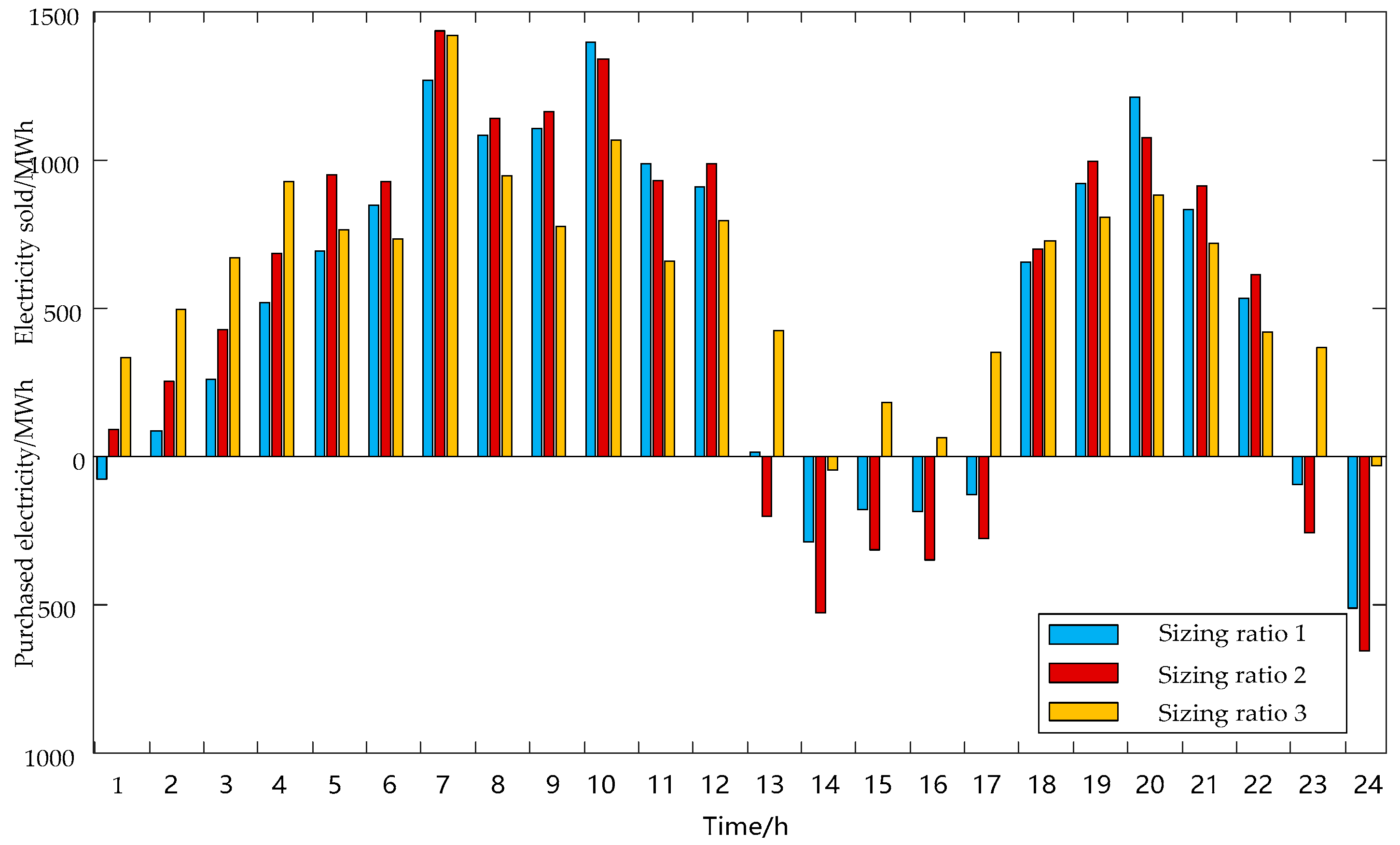
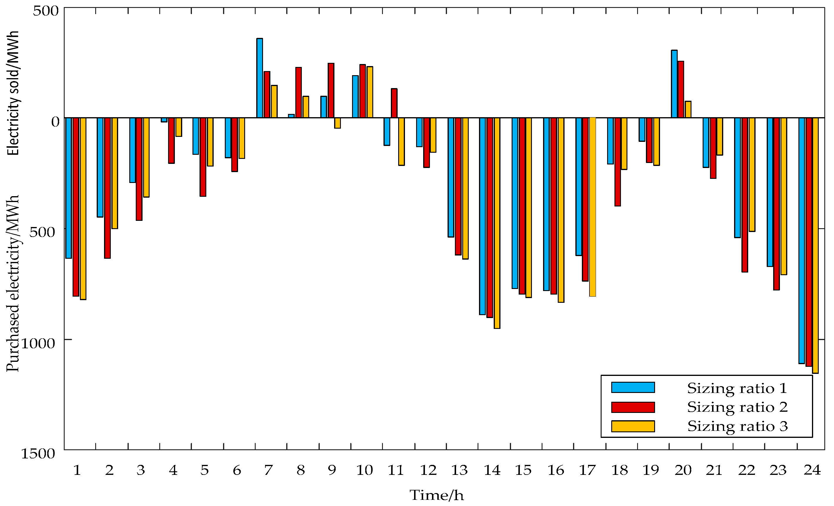
. The output curves of the virtual power plant with different decomposition methods during typical days are shown in Figure 10 and Figure 11. If the generated electricity of the virtual power plant is higher than the local load demand, the rest of the generated electricity can be sold on the spot market; however, if the local load demand cannot be supplied completely by the generated electricity of the virtual power plant, the additional power required by the local load needs to be purchased from the spot market. The purchased electricity and sold electricity of the virtual power plant in the spot market on a typical day during the wet season is shown in Figure 12. The purchased and sold electricity of the virtual power plant on the spot market during a typical day in the dry season is shown in Figure 13. The sales volume is above the horizontal axis, and the purchase amount is below the horizontal axis.

As seen in Figure 10 and Figure 11, regardless of the sizing ratio, in the wet season, the water resources are sufficient, as generated electricity in the wet season is more than that in the dry season. In ratio 1, ratio 2, and ratio 3, the sizing of the hydropower increases in turn, and the generated electricity in the three ratios increases gradually; the output curve with the sizing ratio 1 mode is basically always above the other output curves. During the dry season, water resources are less plentiful, so the output of hydropower is restricted. In this circumstance, the output mainly comes from thermal power. In ratio 1, ratio 2, and ratio 3, the capacity deployment of the thermal power is sequentially reduced, and the total output is sequentially decreased.

From Figure 12 and Figure 13 above, it can be seen that part of the output of the virtual power plant is sold on the spot market during most of the wet period. While, the electricity sold with the ratio 1 mode is less, and the electricity sold with the ratio 3 mode is more.

In most of the dry season, the generated electricity of the virtual power plant is insufficient, so the rest of the electricity demanded by the local load needs to be purchased on the spot market. There are also differences in the purchase of electricity by different schemes. For example, the purchased electricity with ratio 2 and 3 modes is significantly higher than that with ratio 1 in most periods.

Representing a planning problem, the local load will increase in the future, and the growth rate will be different in different scenarios. The sizing scheme is analyzed based on investments and complementary benefits in typical scenarios. Each of the planning years consists of 150 days of wet season and 200 days of dry season.

Based on the sizing method described in this paper, the sizing scheme obtained from the virtual power plant with the maximum annual profit rate for each scheme in the planning year is shown in

Table 7. Sizing growth rate and rate of return of with different complementary modes in the planning year.

Year	Load Growth Rate		Sizing Growth Rate	Rate of Return
				Bv = 0.15, Bf = 0.20, Bg = 0.15			Bv = 0.12, Bf = 0.18, Bg = 0.12			Bv = 0.08, Bf = 0.15, Bg = 0.08
	Wet	Dry
				Sizing Ratio 1	Sizing Ratio 2	Sizing Ratio 3	Sizing Ratio 1	Sizing Ratio 2	Sizing Ratio 3	Sizing Ratio 1	Sizing Ratio 2	Sizing Ratio 3
1	9%	10%	9%	11.23%	11.47%	11.31%	10.90%	11.13%	10.98%	10.51%	10.74%	10.59%
			12%	11.38%	11.71%	11.49%	10.98%	11.30%	11.09%	10.54%	10.85%	10.64%
			15%	11.34%	11.57%	11.39%	10.89%	11.10%	10.94%	10.34%	10.55%	10.39%
2	8%	9%	9%	11.31%	11.63%	11.43%	10.86%	11.17%	10.98%	10.37%	10.66%	10.48%
			12%	11.57%	11.97%	11.74%	11.16%	11.55%	11.33%	10.75%	11.12%	10.90%
			14%	11.38%	11.70%	11.54%	11.04%	11.35%	11.20%	10.62%	10.92%	10.78%
3	8%	8%	8%	11.43%	11.91%	11.54%	10.86%	11.32%	10.97%	10.45%	10.89%	10.55%
			10%	11.70%	12.18%	11.86%	11.23%	11.70%	11.39%	10.78%	11.23%	10.94%
			13%	11.56%	12.03%	11.70%	11.07%	11.53%	11.21%	10.55%	10.98%	10.68%
4	7%	7%	8%	11.54%	12.10%	11.70%	11.08%	11.62%	11.23%	10.53%	11.04%	10.66%
			10%	12.02%	12.34%	12.10%	11.42%	11.72%	11.50%	10.85%	11.14%	10.92%
			13%	11.77%	12.17%	11.93%	11.22%	11.60%	11.37%	10.63%	10.99%	10.78%
5	7%	6%	7%	12.10%	12.43%	12.26%	11.65%	11.98%	11.80%	11.18%	11.50%	11.33%
			10%	11.70%	12.26%	12.18%	11.29%	11.82%	11.76%	10.89%	11.42%	11.34%
			12%	11.62%	12.18%	12.10%	11.26%	11.81%	11.74%	10.93%	11.46%	11.38%

. Meanwhile, it is easily seen that the obtained system yields also have certain differences. When all the load growth rates, capacity growth rates, source complementary indexes, and sizing ratios of hydropower, photovoltaic power, and thermal power are different in typical scenarios, the system yields obtained are changed.

At the same time, the economic results are affected by the complementary indexes. For instance, while the complementary indexes raise continuously, the annual rate of return decreases. Therefore, it is very necessary to choose the appropriate sizing based on the trade-offs between system economics and complementary indexes.

7. Conclusions

In this paper, an innovative sizing method for a virtual power plant is proposed by considering the randomness of photovoltaic output, the seasonality of hydropower output, the spot market price fluctuation, and the mid- to long-term electricity purchase ratios and decomposition. The conclusions are obtained in case study as follows:

• When the spot price is high, the total output of the virtual power plant should be allocated to a lower ratio of a mid- to long-term electricity purchase, and a decomposition method based on spot price should be adopted to obtain a better economic profit.
• Due to the seasonality of hydropower output, profits in dry and wet season are significantly different. When the sizing ratios of hydropower and photovoltaic power decrease, profit in the dry season would increase but decline in the wet season. In order to balance the profit margin between the wet and dry seasons to improve the annual rate of return, the percentage sizing of the hydropower, photovoltaic power, and thermal power sources are recommended to be 25%, 5% and 70%, respectively.
• During the planning years, in order to accommodate the increasing local load, the sizing of the virtual power plant should increase accordingly. A smaller growth rate capacity could not match the load demand and would result in a high cost of electricity purchase on the spot market. However, a larger growth rate of plant capacity could trigger high investment cost and reduce the overall economic planning of system.
• Complementary indexes of the virtual power plant are proposed to increase the system’s profits and become an impact factor to indicate the system’s economics, as high complementary indexes cause low system profit.
• The optimal strategy in the sizing schemes should be determined based on practical requirements with comprehensive consideration of economic and market complementarity.

The impact of water source uncertainty in the hydropower station, the unit combination in the real-time market, and the demand response on sizing will be considered in subsequent research.